Impact of Efficient Driving in Professional Bus Fleets
by
 , , , , ,
Roberto Garcia
1,*, 
Gabriel Diaz
2,
Xabiel G. Pañeda
1,
Alejandro G. Tuero
1,†,
Laura Pozueco
1,
David Melendi
1,
Jose A. Sanchez
1,
Victor Corcoba
1 and
Alejandro G. Pañeda
3 1
Informatics Department, University of Oviedo, 33204 Gijon, Spain
2
Electrical and Computer Engineering Department, Spanish University for Distance Education (UNED), 28040 Madrid, Spain
3
ADN Mobile Solutions, 33394 Gijon, Spain
*
Author to whom correspondence should be addressed.
†
This author is an Industrial Technologies Ph.D. Candidate, at Spanish University for Distance Education (UNED), 28040 Madrid, Spain.
Energies 2017, 10(12), 2060; https://doi.org/10.3390/en10122060
Submission received: 17 October 2017
/
Revised: 16 November 2017
/
Accepted: 29 November 2017
/
Published: 5 December 2017
Abstract
:Diesel engines of the vehicles in the transport sector are responsible for most of the CO2 emissions into the environment. An alternative to reduce fuel consumption is to promote efficient driving techniques. The aim of this paper is to assess the impact of efficient driving on fuel consumption in professional fleets. Data captured from the engine control unit (ECU) of the vehicles are complemented with external information from weather stations and context data from the transport companies. The paper proposes linear and quadratic models in order to quantify the impact of all the terms influencing energy consumption. The analysis was made from the traces captured from a passenger transport company in Spain with more than 50 bus routes. 20 vehicles of five different models were monitored and 58 drivers participated in the study. The results indicate that efficient driving has significant influence on fuel consumption, which confirms efficient driving as a valid and economical option for reducing consumption and therefore emissions of harmful particles into the atmosphere. According to the proposed model, in average external conditions, a driver that increases efficiency from 25% to 75% can reach savings in fuel consumption of up to 16 L/100 km in the analysed bus fleet, which is a significant improvement considering the long distances covered by professionals of the transport sector.
1. Introduction
The improvement of efficient driving techniques has received much attention in recent years. It is well known that one of the main causes of CO2 emissions into the environment is the transport sector [1], meaning that all actions aimed at improving driving techniques and thus reducing fuel consumption gain more relevance. International organizations such as the European Commission have set limits to the increase of CO2 emissions. Thus, they propose to reduce the dependence of Europe on imported fuel and cut carbon emissions in transport by 60% by 2050 [2].
Methods to reduce fuel consumption can be to improve the technology in vehicles, as Kannan et al. [3] with considerable reductions in energy consumption by changing from conventional fuel to bio-fuel. Iodice and Senatore identified the local critical factors that most affect the pollutant emissions in 2-wheel vehicles [4] and proposed cleaner alternative fuels [5]. The authors in [6,7,8,9,10] evaluated the effects of lightweight design in the automotive field as a solution for reducing fuel consumption and the environmental impact of a car. In the same way, Redelbach et al. [11] analysed the impact of weight reduction on the energy consumption by comparing hybrid and a full battery electric vehicle with a conventional car with combustion engine. Driving cycles and electrical vehicles are also investigated in Berzi et al. [12] as a solution to obtain environmental benefits.
Other methods aimed to reduce fuel consumption try to make a more efficient use of the existing technology by optimizing the routes of professional transportation services, by applying maintenance programs or by using efficient driving techniques.
Focusing on professional fleets, of the various alternatives to reduce fuel consumption the most established, both feasibly and economically, is the use of efficient driving techniques [13]. This option takes advantage of the existing fleet without the need to invest in new vehicles and technology. To achieve a significant reduction in fuel consumption and emission of particles to the environment it is necessary to impart proper training programs to the drivers. Drivers control acceleration, braking, speed, rpms, gear position, vehicle position on the road, etc., so their action is critical to achieve significant improvements in environmental efficiency. Moreover, it is necessary to consider that driving is conditioned by external factors such as traffic volume, road maintenance, weather conditions, the planned route, vehicle load, etc. However, fuel consumption does not only depend on driving techniques, there are many other influencing factors. For example, external temperature could influence fuel consumption if it is necessary to activate the air conditioning system. Even in the new vehicles, fuel consumption and extra-emissions increase during the cold transient time due to several factors, such as thermal inefficiency of the engine, partial combustion, catalyst inefficiency and increase of frictions. Likewise, the number of passengers in a bus service increases the load and therefore consumption. Road conditions, traffic lights, the number of stops in a transport service, driving cycle and many other factors can influence energy consumption.
Efficient driving programs oriented towards educating the driver should consider all the mentioned circumstances with the objective of reducing fuel consumption and pollution. Most of these eco-driving courses reduce fuel consumption in the short-term [14], the drivers returning progressively to their habits prior to the training. Rutty et al. [15] evaluated the effect of training in eco-driving in medium sized vehicles. Average emissions of CO2 were reduced by 1.7 kg per vehicle per day. The drivers were only monitored for one month, meaning that this study does not provide any information on long-term behavioural changes. In the same way, Zarkadoula et al. [16] analysed if eco-driving training would enable urban bus drivers to drive in a more economical fashion. Results showed a fuel saving of around 10%. This reduction was only monitored for two months, meaning that the long term effects of eco-driving are not known. Strömberg and Karlsson [17] examined two programmes to develop and maintain ecological bus driving behaviour in Sweden. Fuel saving of 6.8% was obtained. Vagg et al. [18] used a continuous monitoring system to obtain real-time feedback. They obtain a reduction in fuel consumption of 7.61%. However, drivers often revert to their original habits over time.
To solve the short-term problem, Sullman et al. [19] propose the use of simulators to consolidate knowledge on efficient driving after the training courses. They evaluated an eco-driving course for bus drivers which comprised both theoretical and practical elements. They reported a sustained significant reduction in fuel consumption. Six months after training the fuel consumption was 17% lower than before the training. Aimed at private car owners, Barla et al. [20] assesses the impact of an eco-driving training program on fuel consumption for 45 drivers over a period of ten months. They find that eco-driving training induced average city and highway fuel consumption reductions of 4.6% and 2.9% respectively. In Rionda et al. [21] the authors presented a blended learning method which makes use of an on-board tutoring system, an e-learning platform and traditional courses to guide professional drivers to more efficient driving. To evaluate the performance of the learning system, they monitored and analysed the driving of 34 professional drivers over a period of 12 months. The results of the study showed an improvement in driving efficiency and a reduction in fuel consumption of almost 7% compared to the previous year.
Similar to papers about reducing fuel consumption, Ferreira et al. [22] analyse data from a fleet of Lisbon’s public transportation buses over a three-year period. They found that by introducing simple practices, such as optimal clutch use and engine rotation, and avoiding engine idling can reduce consumption on average from 3 to 5 L per 100 km (L/100 km), meaning savings of 30 L per bus per day. Tuero et al. [23] found that the total amount of fuel saved by an urban bus on a route of 12 km with an ideal usage of the inertia would be 3.9 L. Rolim et al. [24] monitored driver behaviour and obtained reductions of 4.8% in fuel consumption with lessons concerning fuel saving.
The aforementioned works present significant savings in fuel consumption in each particular context. They are based on the application of the proposed techniques and the evaluation of the obtained savings. However, the impact of each individual term cannot be quantified and, therefore, it is not feasible to estimate the maximum savings with a combination of driving patterns for the specific context conditions.
Evaluation of an efficient driving process has been based mainly on consumption, as in Caulfield et al. [25] or Zarkadoula et al. [16], without focusing on detecting efficient or inefficient driving behaviours. Nevertheless, Corcoba and Muñoz-Organero [26] have introduced in the analysis the effect of driving patterns. Using the vehicle telemetry, the system detects inefficient areas on a route, warning the user to adjust speed. The set of efficient driving patterns defined in Pozueco et al. [27] has been used in this paper to reveal the action of the driver related to eco-driving. An inefficient performance of driving patterns requires higher levels of acceleration than a proper and efficient execution. In such inefficient driving actions, the enrichment of the air-fuel mixture, outside the optimum range of catalyst efficiency, affects the combustion process and causes higher fuel consumption with a resulting consequence on air quality [28,29].
Regression techniques to study fuel consumption were used in Walnum and Simonsen [30]. They analyse data of a heavy-duty truck transport company and use a set of driving indicators as explanatory variables. They found that, in this context, variables associated with infrastructure and vehicle properties have a greater influence on fuel consumption than driver-influenced variables. In the same way, de Abreu e Silva et al. [31] use regression models to examine fuel consumption in a bus company in Portugal. Fuel consumption was measured for vehicles, drivers and routes. They found that fuel consumption is highly dependent on vehicle type, commercial speed, road gradients of over 5% and bus routes.
The results of the linear model presented in Delgado et al. [32] for a set of five buses showed that average speed, average positive acceleration, and average distance between stops were suitable parameters to predict fuel consumption with reasonable accuracy. The simulation models performed in Demir et al. [33] indicated that consumption varies with size of vehicle, the gradient of the road and speed.
As stated in a complete review of recent research on green road freight transportation by Demir et al. [34], the factors influencing fuel consumption can be divided into five categories: vehicle, environment, traffic, driver and operations. Most fuel consumption models concentrate on vehicle, traffic, and environmental influences, but do not capture driver related issues which are relatively difficult to measure.
Objective of the Paper
The objective of this paper is to determine, using multiple regression analysis, the factors that actually affect efficient driving and calculate their influence. One unsolved problem when studying eco-driving is to distinguish the impact on fuel consumption of the driving action itself and external conditioners such as vehicle load, weather conditions, traffic, etc. Most of the work in this area addresses efficiency based only on fuel consumption without distinguishing between driving patterns and external aspects.
It is also important to consider that the effectiveness of training programs in efficient driving is reduced in the long term. After the training sessions efficiency improves but, without appropriate motivation, drivers progressively abandon good driving habits, gradually returning to the initial situation. A fair, objective and impartial evaluation of the work of the professionals, which includes reward programs based on objective metrics, could help to maintain the effectiveness of the programs of efficient driving in the long term.
Taking into account the aforementioned considerations, one of the most effective measures to evaluate the performance of the driver is to register all the events of the vehicle by capturing information from the Engine Control Unit (ECU) through the Controller Area Network (CAN) bus [35] and store it in a database for later analysis. In this paper, the database system has been enriched with external data from weather services, GPS geolocation from the accelerometer, and additional information provided by the transport companies.
To perform the analysis, a set of real data of 880 drivers of 16 transport companies in Spain and Morocco has been considered. An urban bus company was selected due to the high fuel consumption of these vehicles and the huge number of hours per day they are running, generating an important impact on the environment conditions of the city. The bus company operates in a Spanish city of more than 250,000 inhabitants, and has 50 bus routes. The analysis was done by monitoring the activity of 20 buses of five different models and 58 drivers. From September to December 2015, 94 million traces, 31,181 routes and 41 parameters susceptible of influencing fuel consumption were processed.
The result of the study is an accurate model that quantifies the relationship between fuel consumption and the driving and the external terms considered. The consumption models could contribute to improve training programs of eco-driving. The results of this study allow trainers to emphasize the aspects that really have more influence on eco-driving. Moreover, because the model is able to quantify the relationship between driving actions and fuel consumption, companies can perform a fair and objective evaluation of the professionals which facilitates the inclusion of reward programs.
Finally, results of the performed analysis confirm that improving efficient driving can result in a significant reduction of fuel consumption and, consequently, in environmental improvement in the city in which the professional activity takes place.
This paper is divided into the following sections: The Introduction presents the motivation, literature review, objectives and contributions of the research. Section 2 shows the ideal regression model. Section 3 describes the work methodology and the involved phases to construct the regression models. Section 4 analyses and discusses the results, emphasizing the most important findings. Finally, Section 5 presents the main conclusions.
2. Ideal Regression Model
To implement the model it is necessary to identify the relevant terms that influence fuel consumption. All these terms are the predictor variables in the regression model. Firstly, in this section the ideal regression model is proposed by identifying all the terms that should be part of the analysis, with the objective of reaching the most accurate model that represents the majority of real cases.
The ideal model should include all the information involved in driving such as efficient driving actions that define the driver behaviour, traffic characteristics, infrastructure information, type of transport service and climatic factors during the undertaking of the service. All these terms are included in the ideal model as predictor variables and include the following:
- Efficient driving actions: inertia, idling, acceleration-brake (AB) events, brake-acceleration (BA) events, speed, revolutions per minute (rpm)
- Traffic characteristics: traffic density (high/medium/low), traffic incidences (yes/no)
- Infrastructure characteristics: number of traffic lights, roadworks (yes/no), road surface quality (good/bad), geographic characteristics (positive/negative slope)
- Service characteristics: driver identifier, route identifier, number of service stops, load of the vehicle, type of vehicle, model of the vehicle
- Climatic factors: temperature, rainfall, humidity, pressure, wind speed, wind direction
It should be noted that the ideal model has room for any other factors liable to affect fuel consumption and available for inclusion in the analysis. Thus, subjective information based on drivers, passengers and trainers opinion tests could be included in the model as useful information to improve the quality of the deployed models.
Graphically, the ideal model includes the terms indicated in Figure 1 as predictor variables. The average speed of the service is also indicated as a possible response variable in the case of evaluating this term as output of the model. Obviously, in this case average speed should not be a predictor variable.
3. Work Methodology
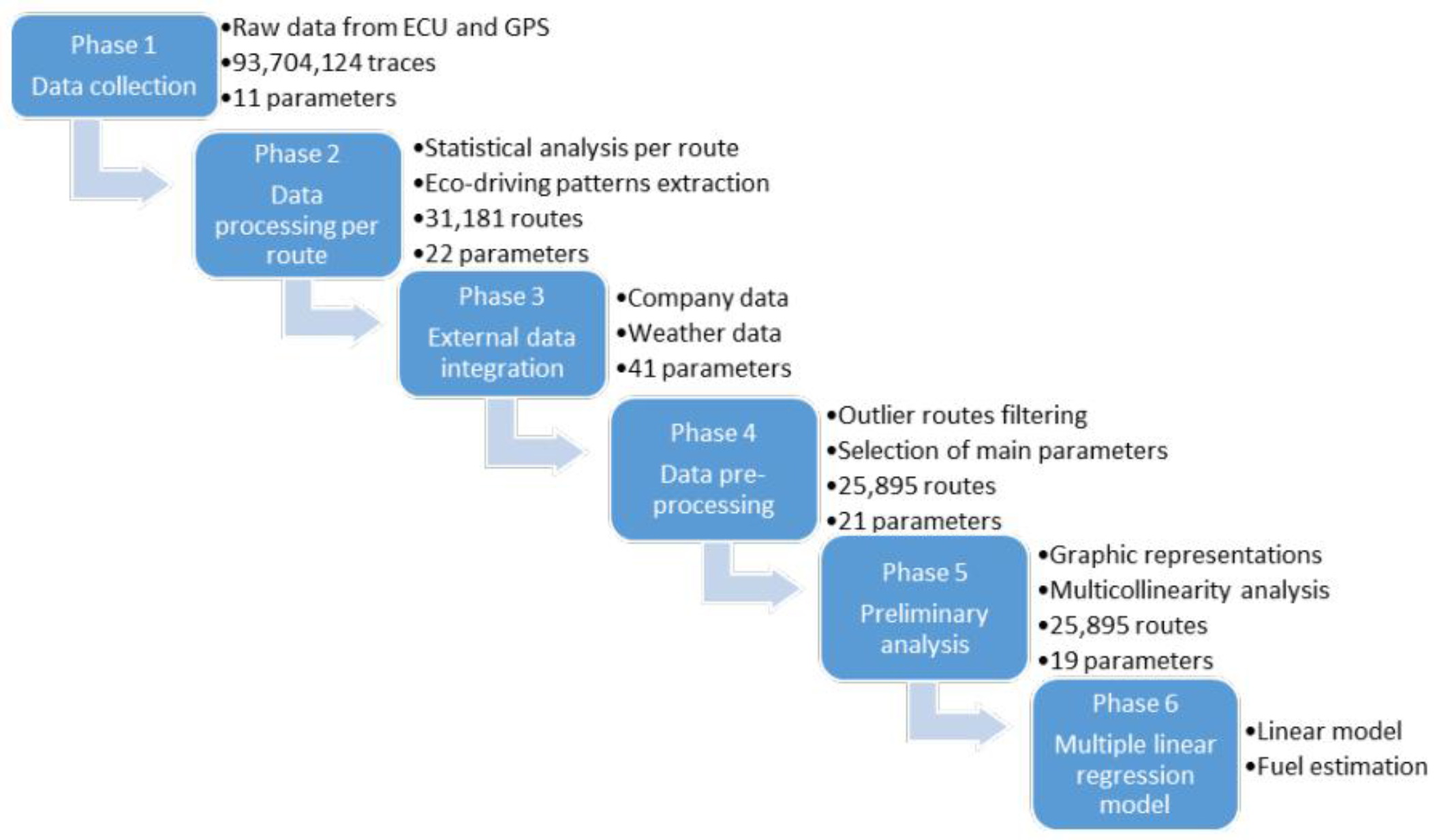
The huge amount of available information to be processed in order to implement the model requires the definition of a work methodology. The performed methodology consists of the phases indicated in Figure 2.
The procedure starts with the capture of raw data from the ECU of the vehicle. These data are statistically processed to obtain the parameters of each route (a bus trip on a specific bus line), such as fuel consumption, speed, rpm and others of interest for the model. Key performance indicators (KPIs) of the defined driving patterns are also calculated in this phase. In phase 3 external data are added to enrich the model, such as weather conditions and data provided by the transport company about the driver, route, type of vehicle and model. In phase 4 all the available information is filtered in order to detect outliers and remove the routes with invalid data from the model. In this phase, the main parameters to include in the final model are also selected. In the next phase, preliminary analyses are performed with graphical representations and basic statistics with the objective of evaluating the viability of the model. It is also necessary to perform a multicollinearity test to discover if there is a strong intercorrelation between independent variables. This test allows us to simplify the model without a loss of accuracy. Finally, the last phase is the implementation of the model using multiple linear regression techniques.
3.1. Phase 1: Data Collection
The study was made from the traces captured from a passenger transport company in Spain with more than 50 bus lines. From September to December 2015 traces were captured from the ECU of 20 vehicles of 5 different models (rigid and articulated). 58 drivers of the company participated in the study covering 10 different bus routes.
The analysis starts with the capture of the data from the ECU by means of an on-board device. The information of the ECU is complemented with geolocation data via GPS and g forces detected with the accelerometer. Then, a trace composed by 11 variables, collected every 1.5 s, is created. The volume of data generated is 94 million traces which contain all the information about the performance of the vehicle and are stored in redundant databases. The parameters of each trace with interest in the study are indicated in Table 1.
3.2. Phase 2: Data Processing Per Route
Taking into account the identifiers of route and vehicle, all the traces of the same route are processed. Thus, for each route is obtained the average fuel consumption (L/100 km), the route duration (s), distance of the route (km), average speed (km/h), maximum speed (km/h), average revolutions (rpm) and maximum revolutions (rpm).
One of the objectives of this work is to determine how driver behaviour influences consumption and, in consequence, environmental quality. The action of the driver, related to eco-driving, is determined by efficient driving patterns [27] that are obtained by processing the traces indicated in the Section 3.1. In this paper, the patterns considered are inertia, idling, acceleration-brake and brake-acceleration. Each pattern is measured and quantified by means of its KPI, as indicated by Parmenter in [36].
3.2.1. Inertia Pattern
Inertia indicates efficiency in driving. Inertia occurs if the vehicle is running with zero consumption. This situation of inertia is produced when the speed is different from zero, a gear is engaged and the accelerator is not pressed. The KPI for the inertia pattern is the percentage of time in inertia in relation to the total duration of the route.
3.2.2. Acceleration-Brake (AB)
The AB pattern characterizes the abuse of the accelerator and brakes. AB pattern look for periods where the driver accelerates during t ≤ 2 s immediately followed by the use of the brakes. As KPI for the AB pattern it is recorded how many times this pattern happens every 100 km.
3.2.3. Brake-Acceleration (BA)
The aim of this pattern is to detect when the driver fails to keep the safety distance, which is both unsafe and inefficient. Every use of the brakes with the intention of stopping the vehicle will be dismissed, while pursuing the hard braking situations (a ≤ −0.882 m/s2) intended to produce an immediate change in speed but without the intention of stopping. As KPI for the BA pattern it is recorded how many times this pattern happens every 100 km.
3.2.4. Idling
Idling has a significant influence on fuel consumption. Idling pattern try to detect periods over a certain amount of time where the vehicle is running but without movement. The KPI for idling is the percentage of time spent idling in relation to the total duration of the route. Table 2 summarizes the conditions and KPI for the selected driving patterns.
3.3. Phase 3: External Data Integration
Additional data is added to the information calculated for each route: data provided by the transport company and weather conditions provided by Spanish State Meteorological Agency (AEMET). As for the weather data, a single point is assumed as representative of the whole city. The information was collected from a weather station located near the city centre. Figure 3 indicates all the available parameters including the information captured by the ECU of the vehicle, the information provided by the transport company and the monitored variables in the weather station.
It is important to point out that the information provided by the transport company is classed as categorical variables, with a limited and fixed number of possible values, some of them with nominal representation such as the bus model or brand. Because these parameters are included in the regression models as predictor variables it is necessary to differentiate between continuous and categorical variables. Categorical variables have a differential treatment in the construction of the model and the explanation of its results.
3.4. Phase 4: Data Pre-Processing and Filtering
Before starting the preliminary analysis for the construction of the model, data processing is performed to detect outliers and eliminate routes that should not become part of the model. Routes with erroneous and invalid values have been eliminated. In this phase the main variables to be included in the model were also selected, trying to avoid redundant information and other intermediate parameters such as those used to calculate the KPI of the driving patterns. The variables included in the model are marked with ‘*’ in Figure 3.
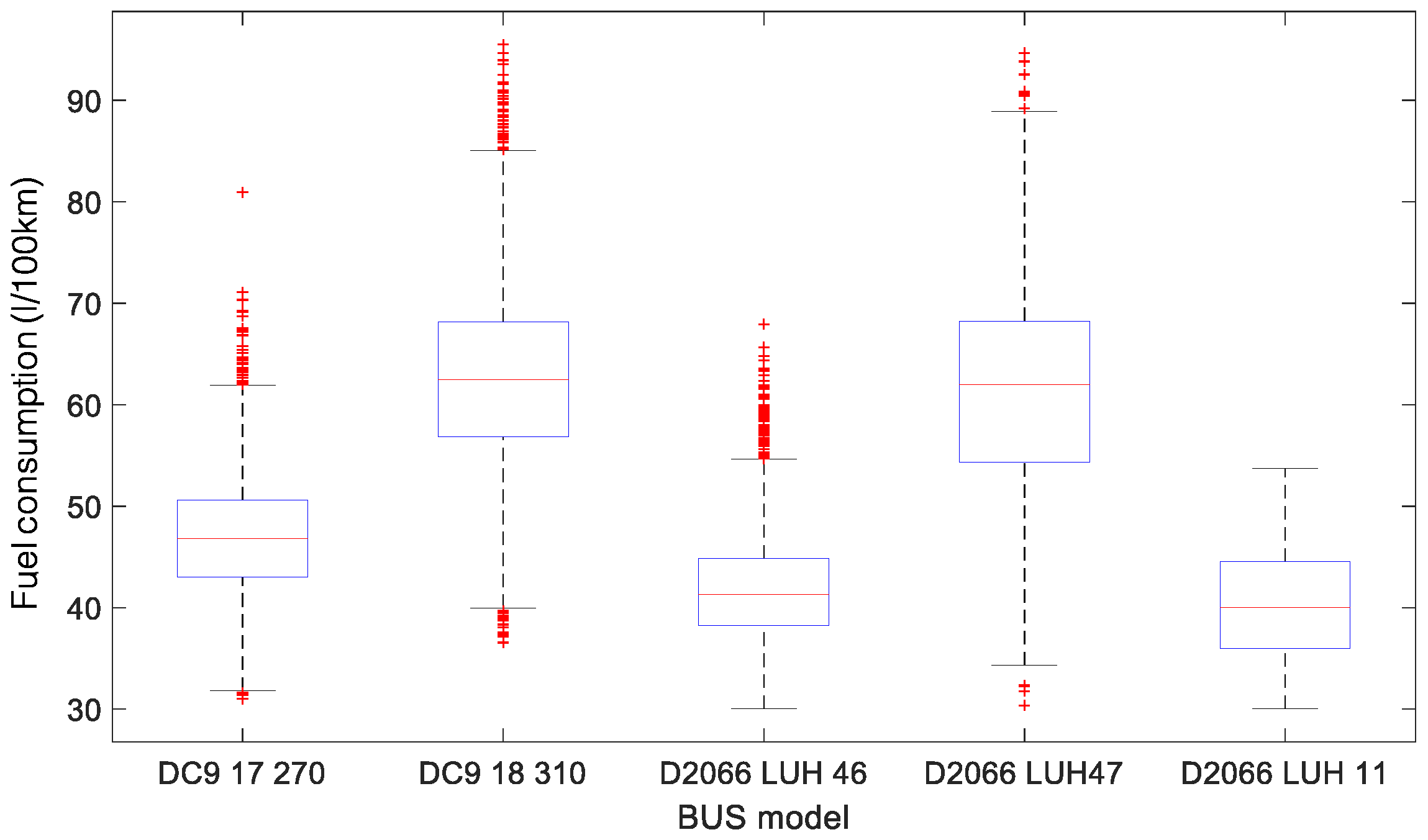
After this process of filtering the model has 25,770 routes and 21 parameters. As stated previously the data correspond to 58 drivers, covering 10 bus routes with 20 vehicles of five different models including both rigid (DC9 17 270, D2066 LUH 11, D2066 LUH 46) and articulated buses (DC9 18 310, D2066 LUH47). In the analysed bus lines, the most used vehicles are D2066 LUH 46 and DC9 18 310, each one with more than 8000 available routes for the analysis.
3.5. Phase 5: Preliminary Analysis
Basic graphic representations were performed to illustrate the relationship between fuel consumption and the variables included in the model. Thus, Figure 4 shows the boxplot of fuel consumption for the 5 bus models, indicating maximum, minimum, median and quartile values for each model. As expected, the bus model influences fuel consumption, the articulated buses, being longer and heavier, showing more fuel consumption than rigid vehicles.
Figure 5 shows the fuel consumption for the different drivers and bus models. As expected, for each bus model consumption changes significantly depending on the driver and a driver can have different consumptions for different bus models.
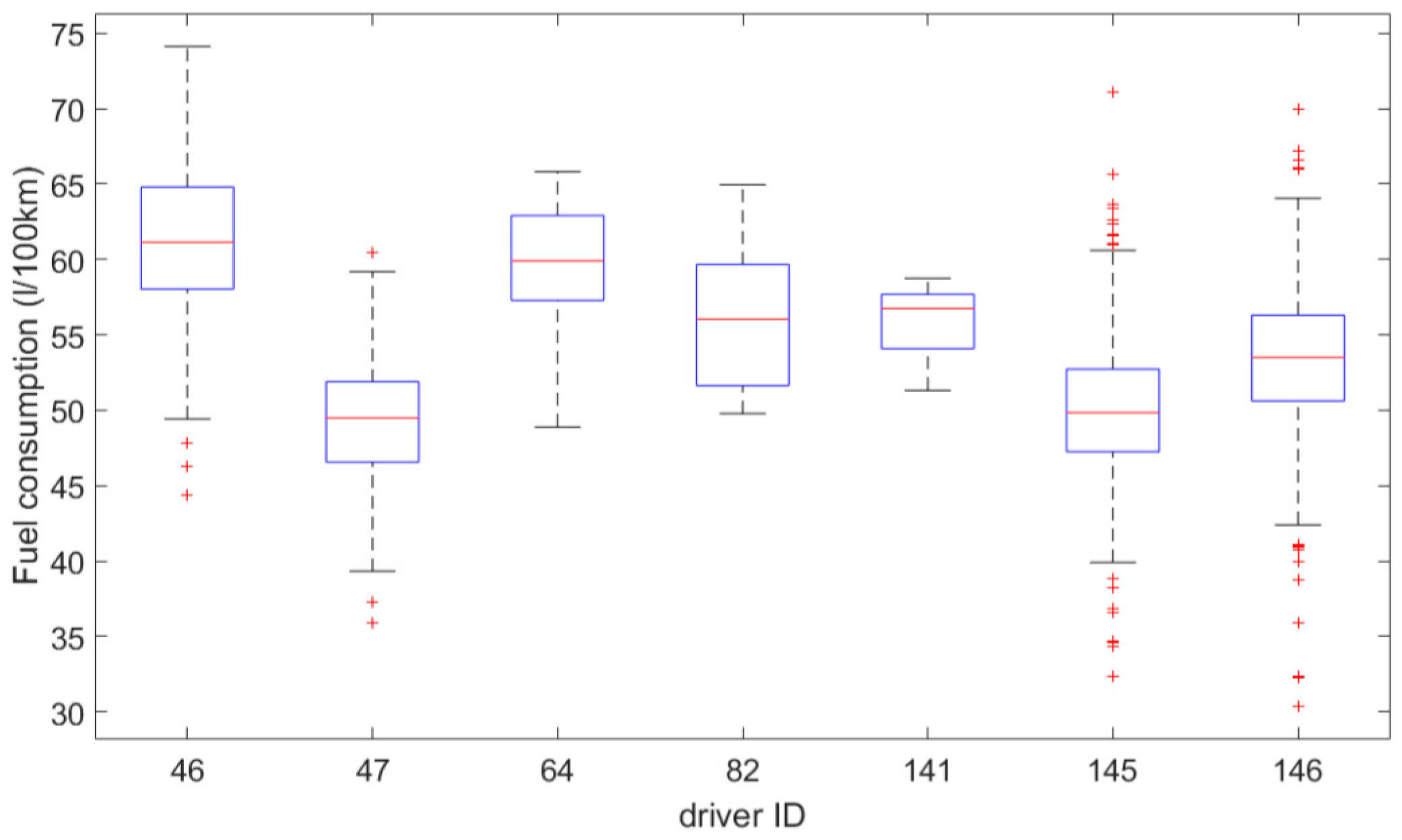
Similarly, the same vehicle and bus line have different consumption depending on the professional driver. As Figure 6 shows, selecting the bus #15 and the route #12 of the company, fuel consumption varies depending on the seven different drivers that cover this route. This could evidence that driver style influences fuel consumption. However, it must be taken into account that other external circumstances can also influence fuel consumption.
Each itinerary (bus route) has its own characteristics such as positive and negative slope, bus stops, traffic lights, traffic volume or number of passengers, making fuel consumption dependent on it. Different vehicles of different models and brands can operate on the same bus route under different external conditions provoking that fuel consumption also depends on all these factors. Results of these preliminary analyses indicate that all the involved variables in this study can influence fuel consumption and, then, justify their inclusion in the proposed models.
Another aspect of crucial importance in this paper is to evaluate if the driving patterns have an impact on fuel consumption. Figure 7a shows how consumption depends on inertia. Because inertia is a pattern of efficiency, the slope of the fitting line suggests that improving driving in inertia reduces fuel consumption. Thus, a simple analysis with the fitting line indicates that, on average, increasing the driving time in inertia by 1%, fuel consumption is reduced 0.24%. Idling, AB and BA are patterns of inefficiency because fuel consumption increases with greater incidence of this patterns, as is verified by the slope of the fitting lines in Figure 7b–d.
A first step in the specification of a model in a multiple regression problem is to identify dependencies between non-categorical predictor variables. Multicollinearity tests have the objective of detecting strong correlation between independent variables. In such cases, some of them should be removed to simplify the model and improve its explanation.
One way to measure multicollinearity is by means of the correlation matrix, which indicates the linear relationship between dependent variables. The correlation matrix is a standard measure of the strength of pairwise linear relationships. Multicollinearity is present when the absolute value of the correlation is larger than 0.6. The correlation matrix was calculated and detected the correlation between predictor variables. As an example, route duration and route distance have a correlation coefficient of 0.628.
Although the correlation matrix measures the strength of pairwise linear relationships among the predictors, its diagnostic value is limited. Correlations only consider pairwise dependencies between predictors. Multicollinearity also appears due to the relationships between arbitrary predictor subsets. In such a case, the variation of a predictor variable is explained by a combination of the other predictors. Variance Inflation Factor (VIF) is useful as a test of multicollinearity and then to detect if there is significant relationship between the independent variables. As stated Mokhtar and Shah in [37], a severe multicollinearity problem exists if VIF > 4. Table 3 shows the VIF for the predictor variables involved.
Results in Table 3 reveal that the variables ‘route_duration’, ‘route_length’ and ‘avg_speed’ have a strong relationship between them and the rest of predictor variables. As expected, route duration is directly related to the length and the average speed. After removing the two variables with greater VIF the revised results are indicated in Table 4.
Although predictor variable ‘KPI AB’ has a VIF value over the threshold of multicollinearity, it is maintained in the model because the main objective of the paper is to analyse the influence of the driving patterns. The complexity of the model does not increase significantly by maintaining this variable and it allows us to know if inefficient driving behaviour by increasing the number of events acceleration-brake has an impact on fuel consumption. With this consideration, all the independent variables in Table 4 will be included as predictor variables in the regression model.
3.6. Phase 6: Multiple Linear Regression Model
Once eliminated multicollinearity between continuous variables, the six categorical variables that could influence fuel consumption (‘driver_id’, ‘line’, ‘direction’, ‘vehicle_id’, ‘BUS_model’, ‘brand’) are added. The regression analysis includes both continuous (12 quantitative terms) and categorical (six qualitative terms) predictor variables. In total the model consists of 18 terms plus the intercept term. For categorical data, dummy variables are constructed. Then, for the ‘driver_id’ predictor variable, driver_id_15 = 1 if the driver #15 is the driver under evaluation and its estimated coefficient will be included in the model. Otherwise, driver_id_15 = 0. For all the categorical variables the same assumption is considered. Table 5 is a summary of the variables used in the regression model.
3.6.1. Linear Model
The simplest model contains an intercept and linear terms for each predictor and the 117 variables, as Equation (1) shows:
For simplicity, all the details about the calculations of the model, residual analyses and other considerations, are shown in Appendix A. The coefficients and statistics of the linear model are indicated in Table A1 (Appendix B). The general characteristics of the linear model are the following:
- Number of observations: 25,529, Error degrees of freedom: 25,419
- Root Mean Squared Error: 3.61
- R-squared: 0.907
- F-statistic vs. constant model: 2260, p-value < 0.01
The coefficient of determination (R-squared) measures the goodness of fit of the model. This coefficient indicates how closely values obtained from fitting a model match the dependent variable the model is intended to predict. The closer to 1 the better the fit. The coefficient of determination is 0.907, suggesting that the model explains 90.7% of the variability in the response variable.
3.6.2. Quadratic Model
Adding new terms can improve the accuracy of the model against an increase in its complexity. A new model which contains an intercept term, linear terms and squared terms was implemented, as indicated in Equation (2):
As with the linear model residuals are analysed to ensure they are randomly and normally distributed, without correlations and independents of the measured values. The model has 31 terms of the 18 predictor variables: intercept term, six linear terms for the categorical predictor variables, 12 linear terms for the continuous predictor variables and 12 quadratic terms for the continuous predictor variables. The general characteristics of the quadratic model are the following:
- Number of observations: 25,565, Error degrees of freedom: 25,443
- Root Mean Squared Error: 3.44
- R-squared: 0.915
- F-statistic vs. constant model: 2270, p-value < 0.01
The quality of the model improves with respect to the linear model, having a lower rmse error and the determination coefficient is 0.915. The complexity of the model does not increase significantly because only the 12 quadratic terms were added respect to the linear model.
3.6.3. Simplified Quadratic Model
Both the linear and quadratic models have several variables with p-value greater than 0.05 indicating that these terms are not significant at the 5% significance level given the other terms. These terms could be removed in order to obtain a simpler model with fewer predictors and similar predictive accuracy.
In this simplified quadratic model, residuals are also analysed and filtered in order to avoid potential problems in the model.
Table A2 (Appendix B) shows the results of the simplified quadratic model, including coefficients of each predictor variable and its related statistics. Due to the simplification, the model consists of 25 terms in 15 predictor variables because no significant terms (BUS model, brand, wind direction) were removed. As Table A2 indicates all the included quadratic terms are significant at the 5% significance level. The general characteristics of the simplified quadratic model are the following:
- Number of observations: 25,568, Error degrees of freedom: 25,450
- Root Mean Squared Error: 3.44
- R-squared: 0.915
- F-statistic vs. constant model: 2350 p-value < 0.01
This simplified model maintains the quality of the quadratic model and reduces complexity by including fewer terms. Of all the analysed models the simplified quadratic model has the best quality and performance to estimate fuel consumption.
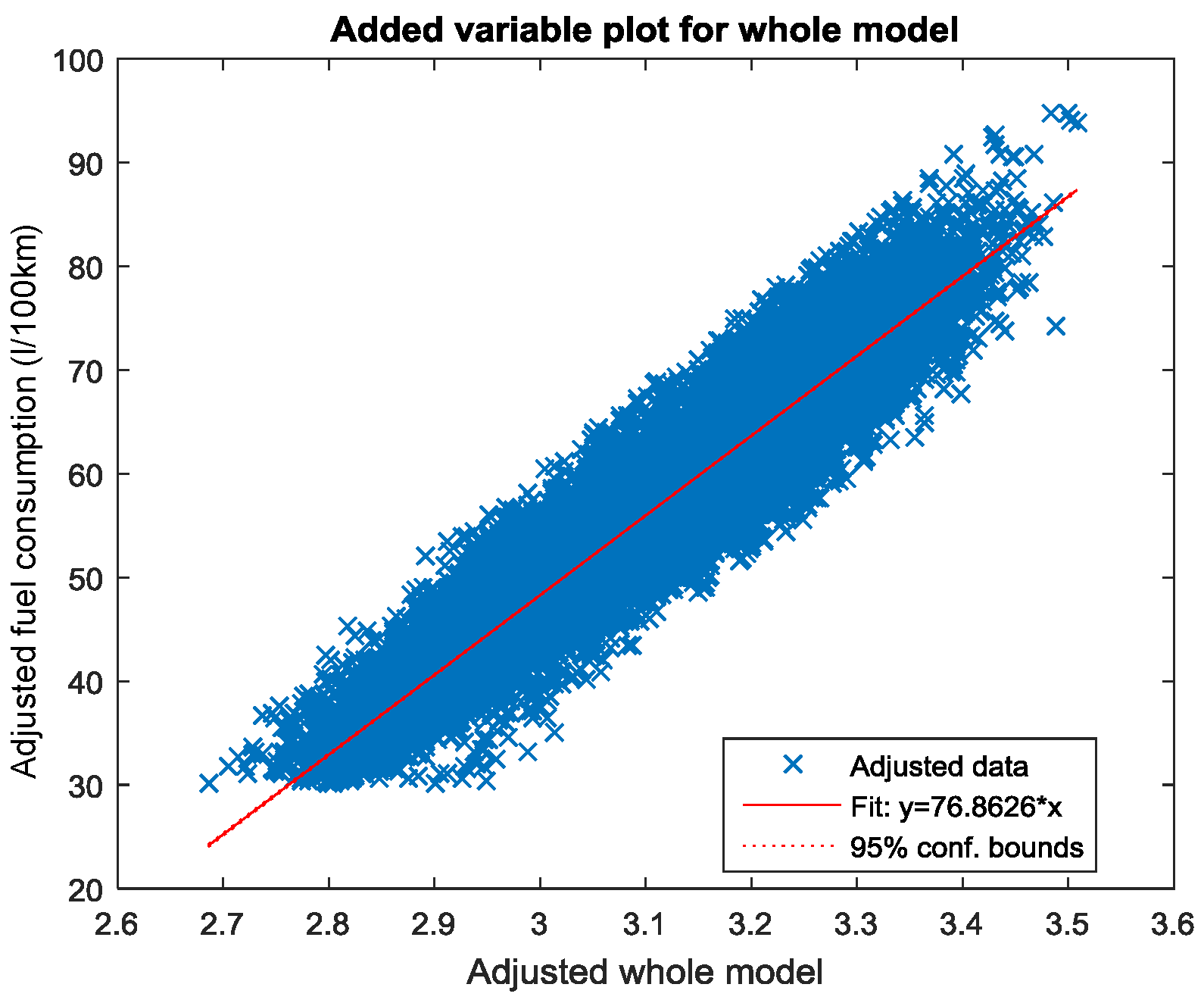
Figure 8 represents the effect of all the predictors on fuel consumption. In this graph, the slope of the red line is the norm of the coefficient vector and, because the 95% confidence bounds do not contain the horizontal line, the model as a whole is very significant.
3.6.4. Model with Interactions
The quality of the model can be improved by including interactions, i.e., product of pairs of different predictors. The new model contains intercept, linear terms, quadratic terms and interactions. The model has R2 = 0.939 but with 1605 variables of 172 terms including interactions. Although quality improves, this model was not considered due to its high complexity.
More complex models, including polynomial with terms of higher degree and product of pairs of distinct predictors were also checked. These models, obviously, improve quality but the improvement is not as significant in relation to the increased complexity of the expressions. Logarithmic models were also checked but the results do not improve those obtained with the linear and quadratic models.
For this reason, the linear and quadratic models permit the best balance between quality and complexity. These models are simplified by removing no significant terms in order to obtain a simpler model with fewer predictors and similar predictive accuracy.
4. Result Analysis and Discussion
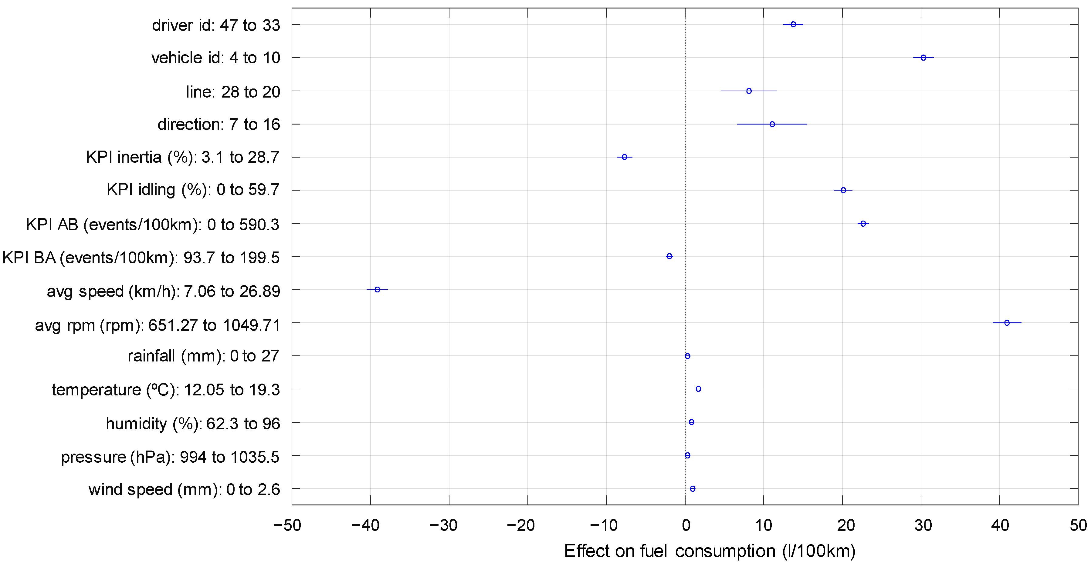
For simplicity in the interpretation of the results, the analysis will focus on the simplified quadratic model. A snapshot of the effect of the predictors on the fuel consumption response is shown in Figure 9. In this plot the predictions come from averaging over the predictors as the one of interest is changed. Horizontal lines indicate 5% confidence intervals.
The information about categorical variables (‘driver id’, ‘vehicle id’, ‘line’, ‘direction’) is not relevant in Figure 9 because these variables are not ordinal and only indicate that fuel consumption is dependent on them, as the model reveals.
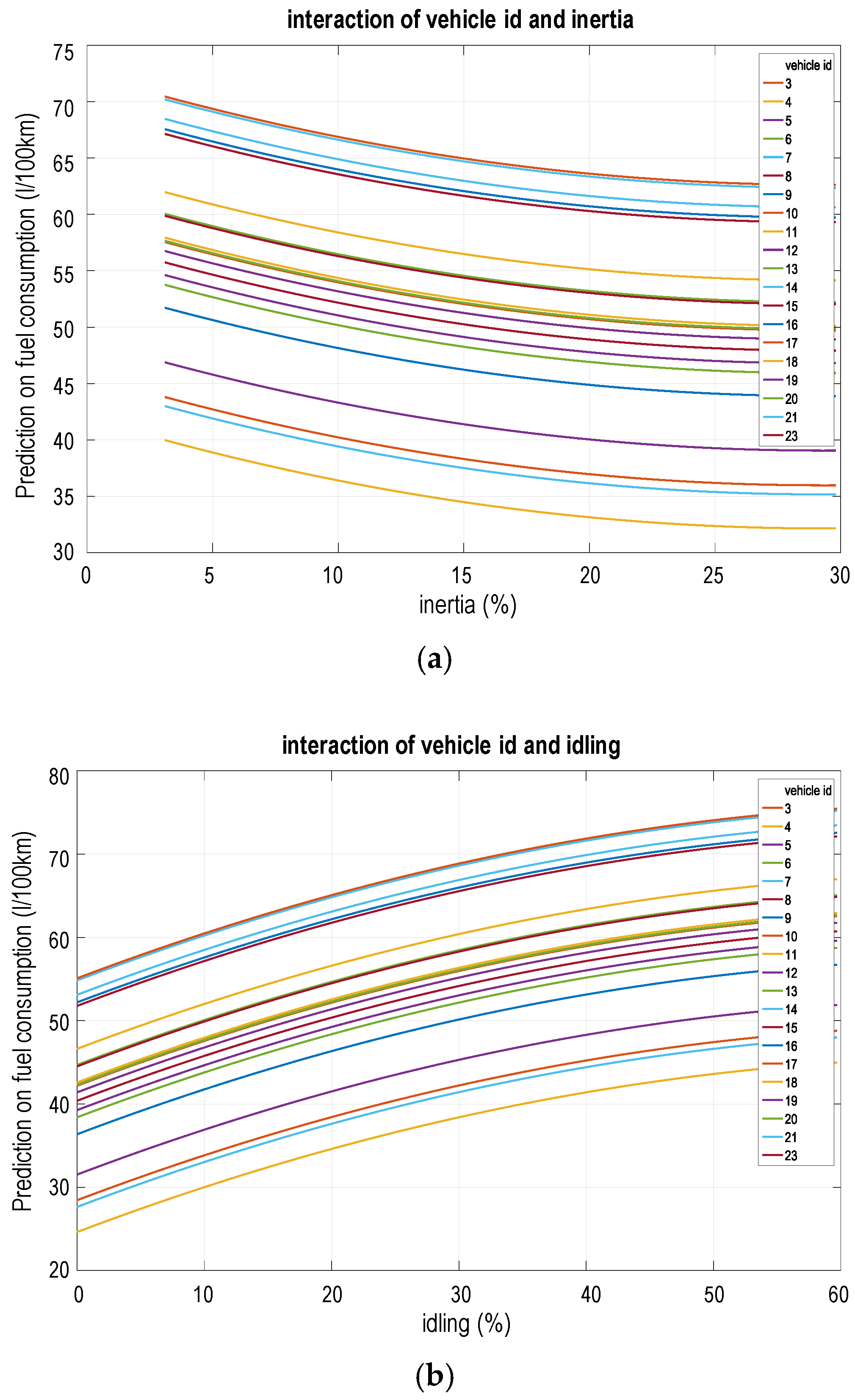
Figure 9 shows that changing inertia from 3.1% to 28.7% fuel consumption decreases by about 9 L/100 km. This result confirms that inertia is one of the most important efficient driving patterns. A more detailed analysis of the inertia for each one of the involved vehicles is indicated in Figure 10a. Firstly, fuel consumption strongly depends on the type of vehicle, articulated vehicles are heavier and, therefore, consume more fuel. Secondly, inertia influences consumption proving that driving with inertia should be considered in order to perform an efficient driving. This is consequent to the leaning of the air-fuel mixture inside the optimum range of catalyst efficiency. As an example, in vehicle #10 (upper line in Figure 10a) fuel consumption decreases from 70 L/100 km to 62 L/100 km by improving the inertia pattern during the route. As can be noticed in the slope of the curves in Figure 10a, savings in fuel consumption are lower for high values of inertia. This could be due to the greater fuel consumption necessary to reach sufficient speed as to drive more than 25% of the time using inertia.
A quantitative explanation is given by analysing the formula of the quadratic model (Equation (2)) and computing the variation of fuel consumption respect the KPI of the inertia (Equation (3)):
being β106 = −0.66922 and β118 = 0.011621 as indicated in Table A2 for the simplified quadratic model. As Equation (3) shows, the variation in fuel consumption depends on the inertia value. Then the savings in fuel consumption changes depending on the work zone in inertia. As an example, let us consider two values of inertia:
KPIinertia = 5%: Δfuel_consumption/ΔKPIinertia = −0.5530 L/%
KPIinertia = 25%: Δfuel_consumption/ΔKPIinertia = −0.0882 L/%
If the driver has an average value of inertia pattern of 5%, savings in fuel consumption are of 0.553 L per each 1% of improvement in inertia, whereas if inertia is 25% savings are of 0.0882 L per each 1% of improvement in inertia.
This feature can be used by trainers to strengthen a more efficient training aspect if the driver already has high values of inertia. On the contrary, if the percentage of driving in inertia is low, the trainer should place special emphasis on this aspect as the benefits in fuel consumption and emission of harmful particles are high in this area of work. Thus, based on Equation (2), with the rest of predictors having their average values, increasing inertia from 5% to 15%, savings in fuel consumption are of 4.36 L/100 km, as Equation (4) reveals:
Idling is an inefficient driving pattern and, as Figure 9 suggests, increasing idling from its minimum to maximum values can result in increasing fuel consumption up to 20 L/100 km. At night with fewer passengers and lower density of traffic, consumption reaches minimum values, whereas during peak hours, with a lot of long service stops to pick up and drop passengers, idling time increases noticeably and, consequently, fuel consumption, as Figure 10b reveals. It is noteworthy that in the majority of cases, idling time is imposed by the type of service and volume of passengers, and is not attributable to inefficient driving. This circumstance should be considered if the company establishes eco-driving policies in order to evaluate efficient driving and implement reward programs.
Looking at the AB driving pattern, both in Figure 9 and Figure 11a an increase in fuel consumption can be seen as the number of AB events increases. AB is a driving pattern of inefficiency and, as such, should be taken into account in training programs due to the impact the pattern has on fuel consumption. Excessive acceleration forces late braking, thereby producing an excess of fuel consumption and a sense of insecurity among passengers.
Meanwhile, the BA driving pattern hardly affects fuel consumption, as shown in Figure 11b. However, BA should be considered in training programs because it impacts significantly the security of driving. Excessive abuse of this pattern indicates that the safety distance with the vehicle in front is insufficient which results in constant braking followed by accelerating to maintain speed. Trainers must take BA into account to improve driving security, although fuel economy is not relevant as shown in the model.
The results of the impact of the average speed are not as initially expected. As Figure 9 indicates, an increase of the average speed from 7 km/h to 26 km/h notably reduces fuel consumption. This could be explained because in itineraries having more accelerating and decelerating phases (e.g., traffic congestion) average speed reduces and fuel consumption is significantly higher.
Regarding rpm the behaviour is as expected. A vehicle running with higher rpm values within the operative range consumes more fuel. Although fuel consumption is related with weather conditions the influence is not significant as is indicated in the average values of Figure 9. These results confirm those suggested in [22] for the fuel consumption in a big city such as Lisbon. Authors concluded that climatic conditions in this city do not impact notably on energy consumption.
As one of the objectives of this paper is to study the impact of driving on fuel consumption numerical estimations are undertaken in order to quantify savings in consumption when driving techniques are improved by means of training programs. Thus, based on the simplified quadratic model and considering, as an example, driver, vehicle, line and direction indicated in Table 6, and average weather conditions from the available real data, fuel consumption is estimated both in efficient and inefficient driving conditions. To avoid extreme results from minimum and maximum values of the variables, driving patterns take the values of quartiles 25 and 75. Quartiles are less sensitive to extreme values and outliers of the variables.
Results in Table 6 reveal the high impact that driving actions have on fuel consumption and in consequence on environmental conditions in the place where the service is deployed. In average context conditions, a driver that increases efficiency from 25% to 75% with the corrective actions in training programs can reach savings of up to 16 L/100 km. This is a very meaningful quantity considering the elevated number of kilometres that a professional of the transport sector covers throughout the whole year. These findings confirm the great economic and environmental benefits achieved with adequate training in efficient driving.
Furthermore, the results of this work validate the proposed driving patterns as indicators of efficiency in driving. Detecting these patterns is key to improve training courses, perform more efficient driving and therefore reduce fuel consumption and the emission of harmful particles into the atmosphere.
5. Conclusions
All the activities focused on reducing fuel consumption in diesel vehicles result in environmental improvements and in costs reduction for transport companies. To implement these improvements an alternative that does not involve large investments is to promote efficient driving techniques among the professionals of the companies. The main problem of this alternative is the difficulty to obtain differentiating knowledge of the factors that influence fuel consumption, because consumption not only depends on driver behaviour but is also related to external variables such as route characteristics, traffic conditions, weather, workload, etc. In this paper, real data from a public transport company have been captured and models of fuel consumption have been deployed using multiple regression techniques.
The implemented models allow us to quantify the impact of the different factors on fuel consumption in a bus fleet, differentiating between those that depend on the driving patterns and those external to the driving. The performed models also permit the validation of the proposed efficient driving patterns as valid tools to influence fuel consumption.
Once known the individual influence of each considered term, the regression models can be used to evaluate the performance of one particular professional in efficient driving by means of fair, objective and quantifiable metrics, avoiding external factors and focusing only on the action of driving. The use of objective metrics makes the implementation of reward programs in the company easier.
Moreover, the results of this work are of special relevance when applying training actions in efficient driving adapted to each professional. Once driving patterns of the driver under evaluation are calculated, training would put more emphasis on those patterns that produce a greater reduction in fuel consumption, always without disregarding training in the remaining driving patterns.
From the output of the model, in average external conditions a driver that increases efficiency from 25% to 75% can reach savings in fuel consumption of up to 16 L/100 km. Taking into account the number of kilometres covered by all the professionals of the company, economic and environmental benefits of employing efficient driving techniques could be noticeable.
The regression models can be improved with the inclusion of new terms that could impact fuel consumption. Thus, it will be useful to capture and integrate variables unavailable in the moment of elaboration of the study, such as traffic density, incidences in the itinerary, traffic lights, roadworks, geographic characteristics of the route and load of the vehicles. The more predictor variables, the greater the accuracy of models and adjustment of the defined efficient driving patterns. New information could permit to perform studies aimed to discover if the driver patterns depend on other circumstances than driving style, such as traffic conditions, distance between stops, etc. Likewise, the use of other modelling techniques could also be useful to improve the accuracy of the predictions, such as the classification and regression trees, KNN (K-Nearest Neighbors) Clustering and Neural Networks.
Future work will be undertaken to apply this knowledge to private vehicles. Considering the defined driving patterns, the objective is to design a recommendation system to provide feedback in real time as an online tutor and guide the driver to perform safe and efficient driving.
Acknowledgments
This work was supported by the Spanish National Research Program (grant number TIN2013-41749-R); Specific R&D&I Agreement between University of Oviedo and HUNOSA (grant number SV-17-HUNOSA-1); and the General Direction of Traffic (DGT) of Spain (grant number SPIP20141277).
Author Contributions
Roberto Garcia conceived the idea of the paper and coordinated all the works; Gabriel Diaz and Xabiel G. Pañeda conceived and designed the experiments; Alejandro G. Tuero and Victor Corcoba analyzed the data; Laura Pozueco and Jose A. Sanchez extracted and organized the data from the database; David Melendi and Alejandro G. Pañeda obtained the data from real vehicles and stored them in the database. Roberto Garcia wrote the paper and David Melendi revised the text. All authors have read, revised and approved the manuscript.
Conflicts of Interest
The authors declare no conflict of interest.
Appendix A. Linear Model
The statistic toolbox of the MatLab software (MathWorks, Natick, MA, USA) was used to implement the regressions. The original model uses 25,770 observations which corresponds to the total number of rows. Model output contains the intercept coefficient (β0) and the coefficients of the predictor variables. The coefficients are estimated so as to minimize the mean squared difference between the prediction vector ŷ = β·f(X) and the true response vector y = fuel_consumption, that is ŷ − y. Maximum likelihood estimation (MLE) is used to estimate the coefficients as it is suitable for dealing with categorical dependent variables [38]. The root mean squared error of the linear model is 3.89. For simplicity, coefficients of this original model are not indicated because it must be adjusted after analysing its residuals.
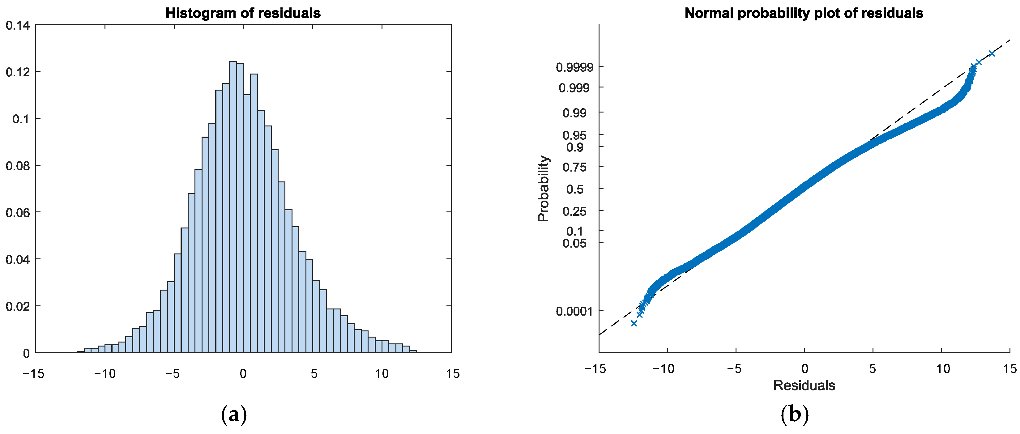
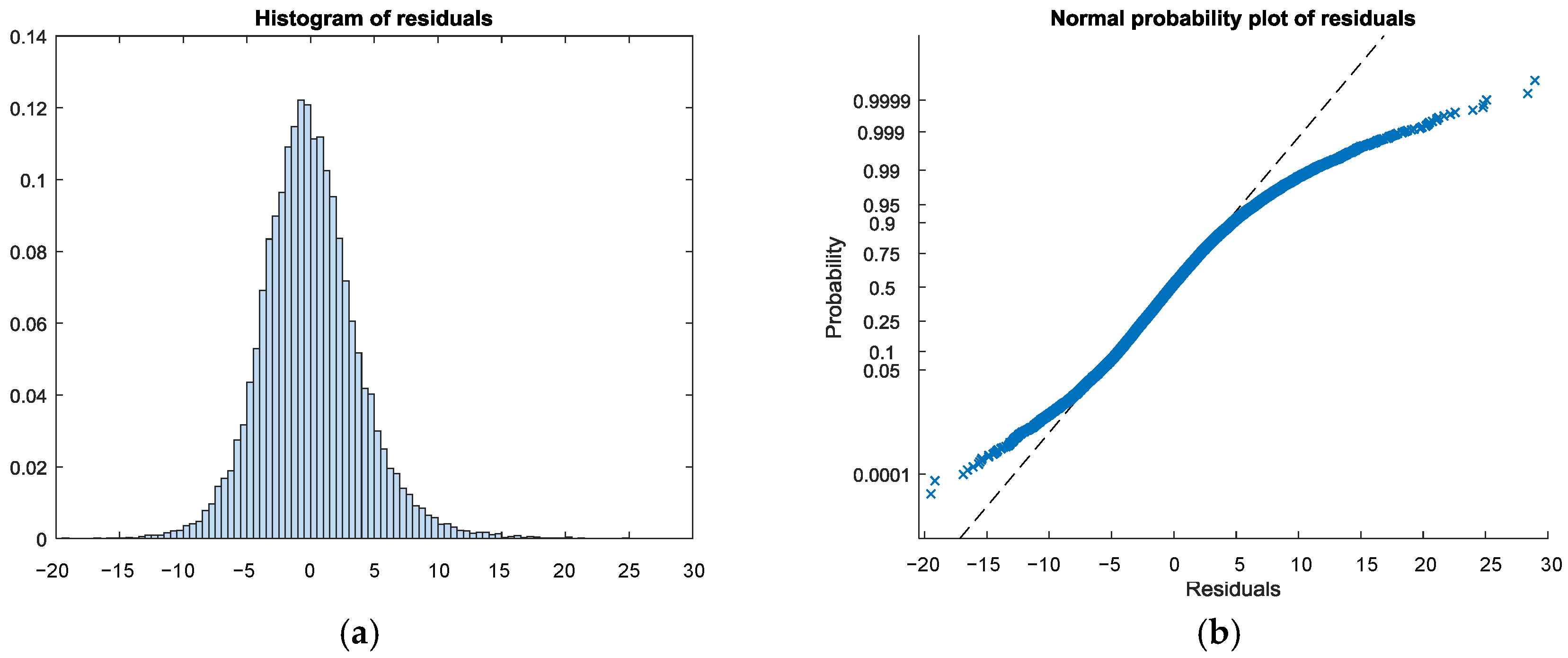
To improve the quality of the linear model, the residuals have to be analysed with the objective of detecting outliers and correlations in the model or in the data. Figure A1a shows the histogram of the residuals and the probability plot, which indicates how the distribution of the residuals compares to a normal distribution with matched variance.
Figure A1.
Plot of residuals for the linear model. (a) Histogram of residuals; (b) Probability plot of residuals.
Figure A1.
Plot of residuals for the linear model. (a) Histogram of residuals; (b) Probability plot of residuals.

Although in the histogram in Figure A1a it appears that residuals follow a normal distribution, the probability plot in Figure A1b shows that the distribution of the residuals differs greatly from the straight line, which means that residuals do not fit to a normal distribution. This situation indicates the presence of outliers in the data. Outliers have been detected and removed (241 outliers in this model) in order to improve the normality of the residuals, obtaining the distribution indicated in Figure A2.
Figure A2.
Plot of residuals for the modified linear model. (a) Histogram of residuals; (b) Probability plot of residuals.
Figure A2.
Plot of residuals for the modified linear model. (a) Histogram of residuals; (b) Probability plot of residuals.
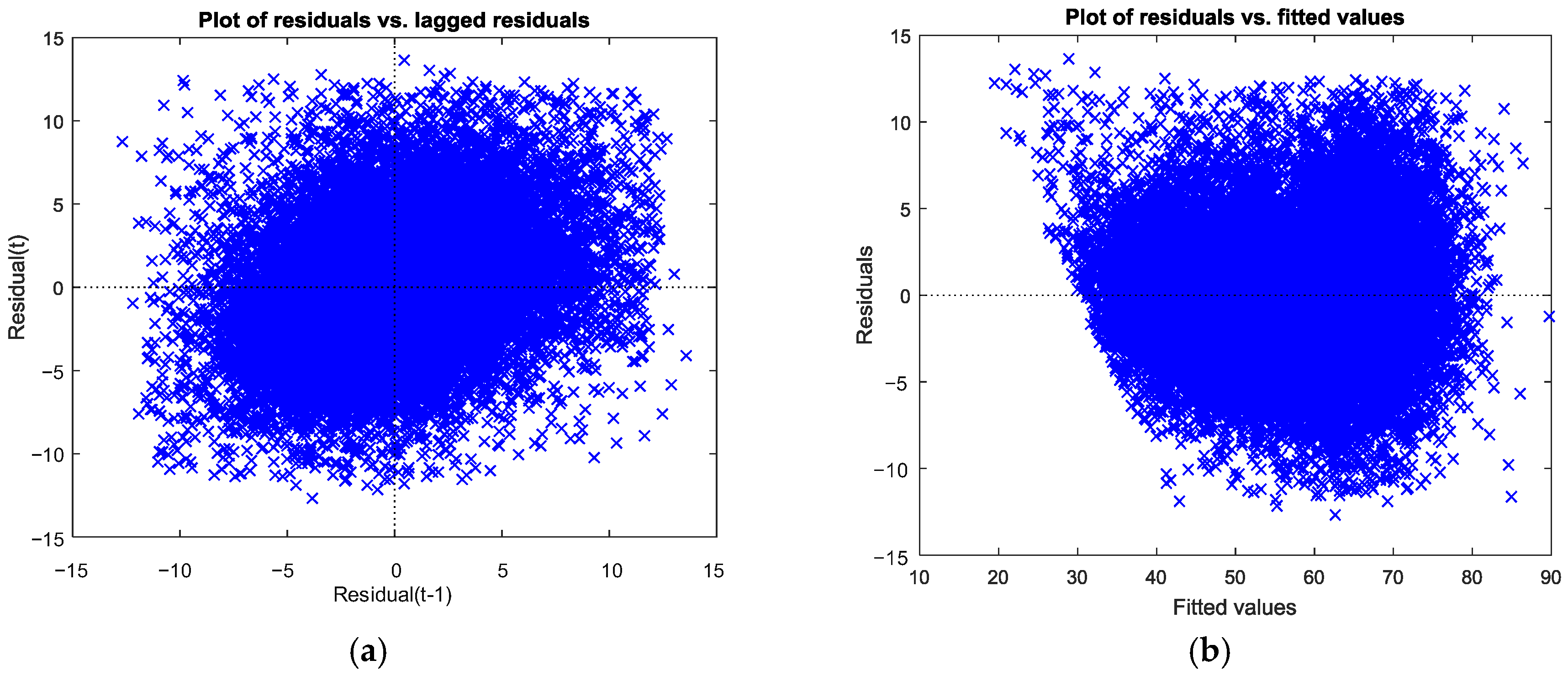
Although residuals have been removed, correlations between them should be analysed in order to evaluate the quality of the model. The scatter plot of Figure A3a shows neither positive nor negative relationship between residuals and lagged residuals, indicating no serial correlation among the residuals.
Figure A3.
Scatter plot of residuals for the linear model. (a) Lagged residuals; (b) Residuals for fitted values.
Figure A3.
Scatter plot of residuals for the linear model. (a) Lagged residuals; (b) Residuals for fitted values.

Moreover, if the model is not well fitted, a clear tendency to have larger residuals for larger fitted values can appear, indicating that the model errors are proportional to the measured values. As Figure A3b indicates, residuals in the model are practically independent of the measured values.
The coefficients of the new linear model are indicated in Table A1 (Appendix B). In Table A1 the first column (under Estimated Coefficients) indicates the terms included in the model. The second column is the Coefficient estimates (βi) for each corresponding term in the model. The standard error of the coefficients is indicated under the SE column. p-value column is of the most important terms because it indicates the p-value for the F-statistic of the hypotheses test that the corresponding coefficient is equal to zero or not. For example, the p-value for the F-statistic for rainfall is greater than 0.05, so this term is not significant at the 5% significance level given the other terms in the model. Other variable predictors have high p-values, indicating that some of these predictors might be unnecessary.
The adjusted model uses 25,529 observations (removing 241 outliers from the initial 25,770 routes). The number of error degrees of freedom is 25,419 because the model has 110 predictors (118 coefficients in Table A1, including the intercept, 8 of them having a 0 value). The root mean squared error is 3.61.
The coefficient of determination R2 is 0.907, suggesting that the model explains 90.7% of the variability in the response variable. Finally, F-statistic has a value of 2260, which is the test statistic for the F-test on the regression model. The p-value for the F-test on the model indicates that the model is significant with a p-value lower than 0.01.
In conclusion, the modified model fits better to the real data than the original linear model, maintaining the same complexity, i.e., the same predictor variables. Adding new terms, such as quadratic or interaction terms (product of pairs of distinct predictors) can improve the accuracy of the model against an increase in its complexity.
Appendix B. Coefficients for the Linear and Simplified Quadratic Models

Table A1.
Coefficient estimation for the modified linear model.
| Coefficient Name | Estimate | SE | p-Value | Coefficient Name | Estimate | SE | p-Value |
|---|---|---|---|---|---|---|---|
| ‘(Intercept)’ | −29.4814 | 4.6128 | <0.0001 | ‘vehicle_id_4’ | −4.1623 | 0.3118 | <0.0001 |
| ‘driver_id_15’ | 0.1584 | 0.8774 | 0.8567 | ‘vehicle_id_5’ | 0 | 0 | NaN |
| ‘driver_id_16’ | −2.2597 | 0.869 | 0.0093 | ‘vehicle_id_6’ | −2.7579 | 0.47 | <0.0001 |
| ‘driver_id_17’ | −1.2998 | 0.9199 | 0.1577 | ‘vehicle_id_7’ | 0.4243 | 0.3685 | 0.2496 |
| ‘driver_id_18’ | 0.8423 | 0.9192 | 0.3595 | ‘vehicle_id_8’ | −1.0246 | 0.3961 | 0.0097 |
| ‘driver_id_19’ | 3.0483 | 0.8434 | 0.0003 | ‘vehicle_id_9’ | 0 | 0 | NaN |
| ‘driver_id_20’ | −0.5468 | 0.8541 | 0.522 | ‘vehicle_id_10’ | 0.947 | 0.3022 | 0.0017 |
| ‘driver_id_22’ | 1.4708 | 0.8725 | 0.0919 | ‘vehicle_id_11’ | 1.0493 | 0.3081 | 0.0007 |
| ‘driver_id_24’ | −2.1395 | 0.7647 | 0.0051 | ‘vehicle_id_12’ | 2.4805 | 0.7514 | 0.001 |
| ‘driver_id_33’ | 5.2847 | 0.8606 | <0.0001 | ‘vehicle_id_13’ | 3.5315 | 0.3854 | <0.0001 |
| ‘driver_id_34’ | −4.642 | 0.8636 | <0.0001 | ‘vehicle_id_14’ | −1.3493 | 0.4695 | 0.0041 |
| ‘driver_id_36’ | −2.0547 | 0.7076 | 0.0037 | ‘vehicle_id_15’ | −3.2132 | 0.2987 | <0.0001 |
| ‘driver_id_37’ | −0.3959 | 0.8301 | 0.6334 | ‘vehicle_id_16’ | −2.0083 | 0.3372 | <0.0001 |
| ‘driver_id_38’ | −0.742 | 0.8159 | 0.3631 | ‘vehicle_id_17’ | 0 | 0 | NaN |
| ‘driver_id_39’ | −0.4396 | 0.8797 | 0.6173 | ‘vehicle_id_18’ | 3.8258 | 0.7786 | <0.0001 |
| ‘driver_id_40’ | −0.4098 | 0.8794 | 0.6412 | ‘vehicle_id_19’ | −1.792 | 0.4326 | <0.0001 |
| ‘driver_id_42’ | 1.0425 | 0.7022 | 0.1377 | ‘vehicle_id_20’ | 0.9992 | 0.3005 | 0.0009 |
| ‘driver_id_43’ | −8.0353 | 0.7008 | <0.0001 | ‘vehicle_id_21’ | 0 | 0 | NaN |
| ‘driver_id_45’ | 4.065 | 0.7198 | <0.0001 | ‘vehicle_id_23’ | 2.7456 | 0.2945 | <0.0001 |
| ‘driver_id_46’ | 0.6387 | 0.6893 | 0.3542 | ‘BUSmodel_DC918310’ | 12.5927 | 0.9042 | <0.0001 |
| ‘driver_id_47’ | −7.9229 | 0.6878 | <0.0001 | ‘BUSmodel_D2066LUH46’ | −0.3407 | 1.5664 | 0.8278 |
| ‘driver_id_48’ | 0.273 | 0.7193 | 0.7043 | ‘BUSmodel_D2066LUH47’ | 15.2586 | 1.4023 | <0.0001 |
| ‘driver_id_49’ | −0.416 | 1.7236 | 0.8093 | ‘BUSmodel_D2066LUH11’ | 0 | 0 | NaN |
| ‘driver_id_54’ | −1.6679 | 0.5231 | 0.0014 | ‘brand_MAN’ | 12.9059 | 1.2537 | <0.0001 |
| ‘driver_id_55’ | −2.4318 | 0.8641 | 0.0049 | ‘line_4’ | −0.8499 | 0.8664 | 0.3266 |
| ‘driver_id_56’ | 4.7764 | 0.8693 | <0.0001 | ‘line_6’ | 2.7434 | 2.3172 | 0.2364 |
| ‘driver_id_58’ | 3.03 | 0.8803 | 0.0006 | ‘line_10’ | −0.4028 | 0.9659 | 0.6766 |
| ‘driver_id_60’ | 0.0733 | 0.835 | 0.9301 | ‘line_12’ | −0.6686 | 0.7631 | 0.3809 |
| ‘driver_id_62’ | −0.6565 | 0.8306 | 0.4293 | ‘line_15’ | 1.4128 | 1.6878 | 0.4026 |
| ‘driver_id_63’ | 0.5477 | 0.8306 | 0.5096 | ‘line_18’ | 1.7276 | 2.9834 | 0.5625 |
| ‘driver_id_64’ | 0.3977 | 0.7167 | 0.579 | ‘line_20’ | 0 | 0 | NaN |
| ‘driver_id_65’ | −2.161 | 0.6898 | 0.0017 | ‘line_28’ | −1.3636 | 1.4092 | 0.3332 |
| ‘driver_id_66’ | −0.618 | 0.6891 | 0.3699 | ‘line_34’ | −2.2839 | 1.3058 | 0.0803 |
| ‘driver_id_71’ | −0.3844 | 0.832 | 0.6441 | ‘direction_2’ | −3.0377 | 0.0601 | <0.0001 |
| ‘driver_id_73’ | −3.882 | 0.7567 | <0.0001 | ‘direction_3’ | −2.8792 | 0.3978 | <0.0001 |
| ‘driver_id_82’ | −1.026 | 0.4571 | 0.0248 | ‘direction_4’ | −2.0758 | 0.3995 | <0.0001 |
| ‘driver_id_83’ | −2.2083 | 0.4564 | <0.0001 | ‘direction_5’ | −1.8565 | 0.3835 | <0.0001 |
| ‘driver_id_86’ | 2.0405 | 0.6965 | 0.0034 | ‘direction_6’ | −2.5327 | 0.37 | <0.0001 |
| ‘driver_id_87’ | −2.0136 | 0.6957 | 0.0038 | ‘direction_7’ | −4.453 | 0.5653 | <0.0001 |
| ‘driver_id_88’ | 1.1148 | 0.6824 | 0.1023 | ‘direction_8’ | −2.0787 | 0.493 | <0.0001 |
| ‘driver_id_89’ | 2.2406 | 0.6837 | 0.0011 | ‘direction_9’ | −1.9207 | 0.44 | <0.0001 |
| ‘driver_id_90’ | 0 | 0 | NaN | ‘direction_10’ | −1.2825 | 0.4607 | 0.0054 |
| ‘driver_id_97’ | −5.8863 | 0.9379 | <0.0001 | ‘direction_11’ | −1.9261 | 1.4817 | 0.1936 |
| ‘driver_id_104’ | −0.2943 | 0.9892 | 0.7661 | ‘direction_12’ | −2.2592 | 1.4819 | 0.1274 |
| ‘driver_id_108’ | −0.4153 | 0.7553 | 0.5824 | ‘direction_13’ | 0 | 0 | NaN |
| ‘driver_id_119’ | −3.6028 | 1.1935 | 0.0025 | ‘direction_14’ | 2.6025 | 2.0087 | 0.1951 |
| ‘driver_id_137’ | 2.5887 | 0.8792 | 0.0032 | ‘direction_15’ | 1.0021 | 2.0837 | 0.6306 |
| ‘driver_id_138’ | −0.7777 | 0.758 | 0.3049 | ‘direction_16’ | 6.7451 | 2.0843 | 0.0012 |
| ‘driver_id_140’ | −0.1618 | 0.2715 | 0.5512 | ‘KPI_inertia’ | −0.5169 | 0.0168 | <0.0001 |
| ‘driver_id_141’ | 1.2446 | 0.7049 | 0.0775 | ‘KPI_idling’ | 0.4826 | 0.0097 | <0.0001 |
| ‘driver_id_142’ | −7.2795 | 0.884 | <0.0001 | ‘KPI_AB’ | 0.0374 | 0.0006 | <0.0001 |
| ‘driver_id_143’ | −1.5906 | 0.8871 | 0.073 | ‘KPI_BA’ | 0.006 | 0.0009 | <0.0001 |
| ‘driver_id_145’ | −7.5521 | 0.6989 | <0.0001 | ‘avg_speed’ | −1.472 | 0.0316 | <0.0001 |
| ‘driver_id_146’ | −4.528 | 0.7009 | <0.0001 | ‘avg_rpm’ | 0.0849 | 0.0023 | <0.0001 |
| ‘driver_id_153’ | −2.5204 | 0.8784 | 0.0041 | ‘rainfall’ | 0.0047 | 0.0066 | 0.4798 |
| ‘driver_id_197’ | 2.3713 | 0.7913 | 0.0027 | ‘temperature’ | 0.1035 | 0.0105 | <0.0001 |
| ‘driver_id_198’ | 1.0048 | 0.8074 | 0.2133 | ‘humidity’ | 0.0124 | 0.0027 | <0.0001 |
| ‘driver_id_221’ | −3.1968 | 0.9759 | 0.0011 | ‘pressure’ | 0.0072 | 0.004 | 0.0762 |
| - | - | - | - | ‘wind_speed’ | 0.3516 | 0.0436 | <0.0001 |
| - | - | - | - | ‘wind_direction’ | 0.001 | 0.0003 | 0.0003 |
Table A2.
Coefficient estimation for the simplified quadratic model.
| Coefficient Name | Estimate | SE | p-Value | Coefficient Name | Estimate | SE | p-Value |
|---|---|---|---|---|---|---|---|
| ‘(Intercept)’ | −182.3003 | 7.5455 | <0.0001 | ‘vehicle_id_7’ | 26.35 | 0.7077 | <0.0001 |
| ‘driver_id_15’ | −0.3614 | 0.8314 | 0.6638 | ‘vehicle_id_8’ | 12.0184 | 0.7996 | <0.0001 |
| ‘driver_id_16’ | −2.5638 | 0.8229 | 0.0018 | ‘vehicle_id_9’ | 7.86 | 1.124 | <0.0001 |
| ‘driver_id_17’ | −2.1333 | 0.8724 | 0.0145 | ‘vehicle_id_10’ | 26.6075 | 0.6873 | <0.0001 |
| ‘driver_id_18’ | 0.4376 | 0.8723 | 0.6159 | ‘vehicle_id_11’ | 14.2664 | 0.813 | <0.0001 |
| ‘driver_id_19’ | 3.3631 | 0.8004 | <0.0001 | ‘vehicle_id_12’ | 3.1339 | 0.717 | <0.0001 |
| ‘driver_id_20’ | 0.3183 | 0.8109 | 0.6947 | ‘vehicle_id_13’ | 16.2018 | 0.8929 | <0.0001 |
| ‘driver_id_22’ | 1.5615 | 0.828 | 0.0593 | ‘vehicle_id_14’ | −0.8011 | 0.4471 | 0.0732 |
| ‘driver_id_24’ | −2.6067 | 0.7297 | 0.0004 | ‘vehicle_id_15’ | 23.3034 | 0.6947 | <0.0001 |
| ‘driver_id_33’ | 5.228 | 0.8167 | <0.0001 | ‘vehicle_id_16’ | 23.6986 | 0.6961 | <0.0001 |
| ‘driver_id_34’ | −5.3319 | 0.8185 | <0.0001 | ‘vehicle_id_17’ | 13.6214 | 0.877 | <0.0001 |
| ‘driver_id_36’ | −1.7222 | 0.675 | 0.0107 | ‘vehicle_id_18’ | 18.0019 | 0.7283 | <0.0001 |
| ‘driver_id_37’ | −0.2969 | 0.7884 | 0.7065 | ‘vehicle_id_19’ | 10.8908 | 0.7809 | <0.0001 |
| ‘driver_id_38’ | −0.4768 | 0.7751 | 0.5385 | ‘vehicle_id_20’ | 13.7631 | 0.862 | <0.0001 |
| ‘driver_id_39’ | −1.2149 | 0.8324 | 0.1445 | ‘vehicle_id_21’ | 24.7905 | 0.6909 | <0.0001 |
| ‘driver_id_40’ | −0.8228 | 0.8318 | 0.3226 | ‘vehicle_id_23’ | 15.9516 | 0.8553 | <0.0001 |
| ‘driver_id_42’ | 0.8535 | 0.67 | 0.2027 | ‘line_4’ | −1.8118 | 0.8023 | 0.0239 |
| ‘driver_id_43’ | −7.8351 | 0.6687 | <0.0001 | ‘line_6’ | 0 | 0 | NaN |
| ‘driver_id_45’ | 4.2385 | 0.6862 | <0.0001 | ‘line_10’ | −2.1015 | 0.8954 | 0.0189 |
| ‘driver_id_46’ | 0.7621 | 0.6586 | 0.2472 | ‘line_12’ | −2.3589 | 0.7007 | 0.0008 |
| ‘driver_id_47’ | −8.5432 | 0.658 | <0.0001 | ‘line_15’ | 1.1505 | 1.5036 | 0.4442 |
| ‘driver_id_48’ | 0.4795 | 0.6854 | 0.4842 | ‘line_18’ | 2.4897 | 2.845 | 0.3815 |
| ‘driver_id_49’ | −1.8543 | 1.6412 | 0.2585 | ‘line_20’ | 4.9141 | 1.2477 | 0.0001 |
| ‘driver_id_54’ | −2.3592 | 0.4987 | <0.0001 | ‘line_28’ | −3.1903 | 1.3397 | 0.0173 |
| ‘driver_id_55’ | −3.0291 | 0.8189 | 0.0002 | ‘line_34’ | 0 | 0 | NaN |
| ‘driver_id_56’ | 3.9202 | 0.8249 | <0.0001 | ‘direction_2’ | −2.7345 | 0.0578 | <0.0001 |
| ‘driver_id_58’ | 1.7355 | 0.8345 | 0.0376 | ‘direction_3’ | −1.8296 | 0.3791 | <0.0001 |
| ‘driver_id_60’ | 0.9378 | 0.7921 | 0.2364 | ‘direction_4’ | −0.8584 | 0.3805 | 0.0241 |
| ‘driver_id_62’ | −0.2809 | 0.789 | 0.7219 | ‘direction_5’ | −1.0078 | 0.3646 | 0.0057 |
| ‘driver_id_63’ | 0.7057 | 0.7894 | 0.3713 | ‘direction_6’ | −1.3642 | 0.3521 | 0.0001 |
| ‘driver_id_64’ | 0.89 | 0.6839 | 0.1931 | ‘direction_7’ | −3.1022 | 0.5395 | <0.0001 |
| ‘driver_id_65’ | −2.7074 | 0.6582 | <0.0001 | ‘direction_8’ | −1.4307 | 0.4712 | 0.0024 |
| ‘driver_id_66’ | −0.196 | 0.6588 | 0.766 | ‘direction_9’ | −1.1001 | 0.4174 | 0.0084 |
| ‘driver_id_71’ | −0.0016 | 0.789 | 0.9984 | ‘direction_10’ | −0.8129 | 0.4384 | 0.0637 |
| ‘driver_id_73’ | −4.1684 | 0.7225 | <0.0001 | ‘direction_11’ | −1.287 | 1.678 | 0.4431 |
| ‘driver_id_82’ | −2.2082 | 0.437 | <0.0001 | ‘direction_12’ | −1.5262 | 1.6778 | 0.363 |
| ‘driver_id_83’ | −2.6447 | 0.4348 | <0.0001 | ‘direction_13’ | 1.0217 | 2.1264 | 0.6309 |
| ‘driver_id_86’ | 2.3208 | 0.6645 | 0.0005 | ‘direction_14’ | 3.7348 | 1.0591 | 0.0004 |
| ‘driver_id_87’ | −1.446 | 0.6645 | 0.0296 | ‘direction_15’ | 0.908 | 2.192 | 0.6787 |
| ‘driver_id_88’ | 0.9978 | 0.652 | 0.1259 | ‘direction_16’ | 7.9745 | 2.1914 | 0.0003 |
| ‘driver_id_89’ | 1.8575 | 0.6525 | 0.0044 | ‘KPI_inertia’ | −0.6692 | 0.0559 | <0.0001 |
| ‘driver_id_90’ | 0 | 0 | NaN | ‘KPI_idling’ | 0.5875 | 0.0239 | <0.0001 |
| ‘driver_id_97’ | −6.0344 | 0.8908 | <0.0001 | ‘KPI_AB’ | 0.0234 | 0.0013 | <0.0001 |
| ‘driver_id_104’ | 0.385 | 0.9347 | 0.6804 | ‘KPI_BA’ | 0.0327 | 0.0023 | <0.0001 |
| ‘driver_id_108’ | −1.4376 | 0.72 | 0.0459 | ‘avg_speed’ | −5.3909 | 0.085 | <0.0001 |
| ‘driver_id_119’ | −2.5193 | 1.1391 | 0.027 | ‘avg_rpm’ | 0.5366 | 0.0152 | <0.0001 |
| ‘driver_id_137’ | 1.5513 | 0.8348 | 0.0631 | ‘rainfall’ | 0.0111 | 0.0063 | 0.0782 |
| ‘driver_id_138’ | −1.2218 | 0.7233 | 0.0912 | ‘temperature’ | −0.7529 | 0.0652 | <0.0001 |
| ‘driver_id_140’ | −0.8873 | 0.2614 | 0.0007 | ‘humidity’ | −0.0893 | 0.022 | 0.0001 |
| ‘driver_id_141’ | 1.3852 | 0.672 | 0.0393 | ‘pressure’ | 0.0072 | 0.0039 | 0.0609 |
| ‘driver_id_142’ | −7.6304 | 0.8359 | <0.0001 | ‘wind_speed’ | 0.7559 | 0.1152 | <0.0001 |
| ‘driver_id_143’ | −2.0991 | 0.8383 | 0.0123 | ‘KPI_inertia^2’ | 0.0116 | 0.002 | <0.0001 |
| ‘driver_id_145’ | −7.4583 | 0.6688 | <0.0001 | ‘KPI_idling^2’ | −0.0042 | 0.0004 | <0.0001 |
| ‘driver_id_146’ | −4.895 | 0.6697 | <0.0001 | ‘KPI_AB^2’ | <0.0001 | <0.0001 | <0.0001 |
| ‘driver_id_153’ | −2.7698 | 0.8326 | 0.0009 | ‘KPI_BA^2’ | −0.0002 | <0.0001 | <0.0001 |
| ‘driver_id_197’ | 0.6281 | 0.7571 | 0.4067 | ‘avg_speed^2’ | 0.1006 | 0.002 | <0.0001 |
| ‘driver_id_198’ | 0.3363 | 0.7766 | 0.665 | ‘avg_rpm^2’ | −0.0003 | <0.0001 | <0.0001 |
| ‘driver_id_221’ | −3.2991 | 0.9268 | 0.0004 | ‘temperature^2’ | 0.0313 | 0.0024 | <0.0001 |
| ‘vehicle_id_4’ | −3.6972 | 0.2976 | <0.0001 | ‘humidity^2’ | 0.0007 | 0.0001 | <0.0001 |
| ‘vehicle_id_5’ | 13.1325 | 0.858 | <0.0001 | ‘wind_speed^2’ | −0.1417 | 0.0495 | 0.0042 |
| ‘vehicle_id_6’ | 10.0102 | 0.766 | <0.0001 | - | - | - | - |
References
- Jochem, P.; Rothengatter, W.; Schade, W. Climate change and transport. Transp. Res. Part Transp. Environ. 2016, 45, 1–3. [Google Scholar] [CrossRef]
- European Commission Roadmap to a Single European Transport Area: Towards a Competitive and Resource-Efficient Transport System. Available online: http://eur-lex.europa.eu/legal-content/EN/TXT/?uri=URISERV%3Atr0054 (accessed on 15 September 2016).
- Kannan, N.; Saleh, A.; Osei, E. Estimation of energy consumption and greenhouse gas emissions of transportation in beef cattle production. Energies 2016, 9, 960. [Google Scholar] [CrossRef]
- Senatore, A.; Iodice, P. Road transport emission inventory in a regional area by using experimental two-wheelers emission factors. In Lecture Notes in Engineering and Computer Science, Proceedings of the World Congress on Engineering, London, UK, 3–5 July 2013; International Association of Engineers (IAENG): London, UK, 2013; pp. 681–685. [Google Scholar]
- Iodice, P.; Senatore, A. Influence of Ethanol-Gasoline Blended Fuels on Cold Start Emissions of a Four-Stroke Motorcycle. Methodology and Results; SAE Technical Paper: Warrendale, PA, USA, 2013. [Google Scholar]
- Del Pero, F.; Delogu, M.; Pierini, M. The effect of lightweighting in automotive LCA perspective: Estimation of mass-induced fuel consumption reduction for gasoline turbocharged vehicles. J. Clean. Prod. 2017, 154, 566–577. [Google Scholar] [CrossRef]
- Delogu, M.; Del Pero, F.; Pierini, M. Lightweight design solutions in the automotive field: Environmental modelling based on fuel reduction value applied to diesel turbocharged vehicles. Sustainability 2016, 8, 1167. [Google Scholar] [CrossRef]
- Koffler, C.; Rohde-Brandenburger, K. On the calculation of fuel savings through lightweight design in automotive life cycle assessments. Int. J. Life Cycle Assess. 2010, 15, 128–135. [Google Scholar] [CrossRef]
- Kelly, J. C.; Sullivan, J.L.; Burnham, A.; Elgowainy, A. Impacts of vehicle weight reduction via material substitution on life-cycle greenhouse gas emissions. Environ. Sci. Technol. 2015, 49, 12535–12542. [Google Scholar] [CrossRef] [PubMed]
- Kim, H.C.; Wallington, T.J.; Sullivan, J.L.; Keoleian, G.A. Life cycle assessment of vehicle lightweighting: novel mathematical methods to estimate use-phase fuel consumption. Environ. Sci. Technol. 2015, 49, 10209–10216. [Google Scholar] [CrossRef] [PubMed]
- Redelbach, M.; Klötzke, M.; Horst, E.F. Impact of Lightweight Design on Energy Consumption and Cost Effectiveness of Alternative Powertrain Concepts. In Proceedings of the European Electric Vehicle Congress (EEVC), Brüssel, Belgium, 19–22 November 2012; pp. 1–9. [Google Scholar]
- Berzi, L.; Delogu, M.; Pierini, M. Development of driving cycles for electric vehicles in the context of the city of Florence. Transp. Res. Part D 2016, 47, 299–322. [Google Scholar] [CrossRef]
- Barkenbus, J.N. Eco-driving: An overlooked climate change initiative. Energy Policy 2010, 38, 762–769. [Google Scholar] [CrossRef]
- Andrieu, C.; Pierre, G.S. Comparing effects of eco-driving training and simple advices on driving behavior. Procedia Soc. Behav. Sci. 2012, 54, 211–220. [Google Scholar] [CrossRef]
- Rutty, M.; Matthews, L.; Andrey, J.; Matto, T.D. Eco-driver training within the city of calgary’s municipal fleet: Monitoring the impact. Transp. Res. Part D 2013, 24, 44–51. [Google Scholar] [CrossRef]
- Zarkadoula, M.; Zoidis, G.; Tritopoulou, E. Training urban bus drivers to promote smart driving: A note on a Greek eco-driving pilot program. Transp. Res. Part D 2007, 12, 449–451. [Google Scholar] [CrossRef]
- Strömberg, H.K.; Karlsson, I.C.M. Comparative effects of eco-driving initiatives aimed at urban bus drivers—Results from a field trial. Transp. Res. Part D 2013, 22, 28–33. [Google Scholar] [CrossRef]
- Vagg, C.; Brace, C.J.; Hari, D.; Akehurst, S.; Poxon, J.; Ash, L. Development and field trial of a driver assistance system to encourage eco-driving in light commercial vehicle fleets. IEEE Trans. Intell. Transp. Syst. 2013, 14, 796–805. [Google Scholar] [CrossRef] [Green Version]
- Sullman, M.J.M.; Dorn, L.; Niemi, P. Eco-driving training of professional bus drivers—Does it work? Transp. Res. Part C 2015, 58, 749–759. [Google Scholar] [CrossRef]
- Barla, P.; Gilbert-Gonthier, M.; Lopez Castro, M.A.; Miranda-Moreno, L. Eco-driving training and fuel consumption: Impact, heterogeneity and sustainability. Energy Econ. 2017, 62, 187–194. [Google Scholar] [CrossRef]
- Rionda, A.; Pañeda, X.G.; García, R.; Díaz, G.; Martínez, D.; Mitre, M.; Arbesú, D.; Marín, I. Blended learning system for efficient professional driving. Comput. Educ. 2014, 78, 124–139. [Google Scholar] [CrossRef]
- Ferreira, J.C.; de Almeida, J.; da Silva, A.R. The impact of driving styles on fuel consumption: A data-warehouse-and-data-mining-based discovery process. IEEE Trans. Intell. Transp. Syst. 2015, 16, 2653–2662. [Google Scholar] [CrossRef]
- Tuero, A.G.; Pozueco, L.; García, R.; Díaz, G.; Pañeda, X.G.; Melendi, D.; Rionda, A.; Martínez, D. Economic impact of the use of inertia in an urban bus company. Energies 2017, 10, 1029. [Google Scholar] [CrossRef]
- Rolim, C.C.; Baptista, P.C.; Duarte, G.O.; Farias, T.L. Impacts of on-board devices and training on light duty vehicle driving behavior. Procedia Soc. Behav. Sci. 2014, 111, 711–720. [Google Scholar] [CrossRef]
- Caulfield, B.; Brazil, W.; Ni Fitzgerald, K.; Morton, C. Measuring the success of reducing emissions using an on-board eco-driving feedback tool. Transp. Res. Part D 2014, 32, 253–262. [Google Scholar] [CrossRef]
- Corcoba Magaña, V.; Muñoz-Organero, M. Discovering regions where users drive inefficiently on regular journeys. IEEE Trans. Intell. Transp. Syst. 2015, 16, 221–234. [Google Scholar] [CrossRef]
- Pozueco, L.; Tuero, A.G.; Pañeda, X.G.; Melendi, D.; García, R.; Pañeda, A.G.; Rionda, A.; Díaz, G.; Mitre, M. Adaptive learning for efficient driving in urban public transport. In Proceedings of the International Conference on Computer, Information and Telecommunication Systems (CITS), Gijon, Spain, 15–17 July 2015; pp. 1–5. [Google Scholar]
- Iodice, P.; Senatore, A. Exhaust emissions of new high-performance motorcycles in hot and cold conditions. Int. J. Environ. Sci. Technol. 2015, 12, 3133–3144. [Google Scholar] [CrossRef]
- Iodice, P.; Senatore, A. Analysis of a Scooter Emission Behavior in Cold and Hot Conditions: Modelling and Experimental Investigations; SAE Technical Paper: Warrendale, PA, USA, 2012. [Google Scholar]
- Walnum, H.J.; Simonsen, M. Does driving behavior matter? An analysis of fuel consumption data from heavy-duty trucks. Transp. Res. Part D 2015, 36, 107–120. [Google Scholar] [CrossRef]
- de Abreu e Silva, J.; Moura, F.; Garcia, B.; Vargas, R. Influential vectors in fuel consumption by an urban bus operator: Bus route, driver behavior or vehicle type? Transp. Res. Part D 2015, 38, 94–104. [Google Scholar] [CrossRef]
- Delgado, O.F.; Clark, N.N.; Thompson, G.J. Modeling transit bus fuel consumption on the basis of cycle properties. J. Air Waste Manag. Assoc. 2011, 61, 443–452. [Google Scholar] [CrossRef] [PubMed]
- Demir, E.; Bektaş, T.; Laporte, G. A comparative analysis of several vehicle emission models for road freight transportation. Transp. Res. Part D 2011, 16, 347–357. [Google Scholar] [CrossRef]
- Demir, E.; Bektaş, T.; Laporte, G. A review of recent research on green road freight transportation. Eur. J. Oper. Res. 2014, 237, 775–793. [Google Scholar] [CrossRef]
- Di Natale, M.; Zeng, H.; Giusto, P.; Ghosal, A. Understanding and Using the Controller Area Network Communication Protocol; Springer: New York, NY, USA, 2012. [Google Scholar]
- Parmenter, D. Key Performance Indicators (KPI): Developing, Implementing, and Using Winning KPIs; John Wiley & Sons: Hoboken, NJ, USA, 2010. [Google Scholar]
- Mokhtar, K.; Shah, M.Z. A Regression Model for Vessel Turnaround Time; Tokyo Academic, Industry & Cultural Integration Tour 2006; Shibaura Institute of Technology: Tokyo, Japan, 2016; pp. 1–15. [Google Scholar]
- Yadlin-Weintraub, M. Some procedures for the statistical and empirical analyses of probabilistic discrete decisions models. Transp. Res. Part B 1991, 25, 215–236. [Google Scholar] [CrossRef]
Figure 1.
Ideal regression model.
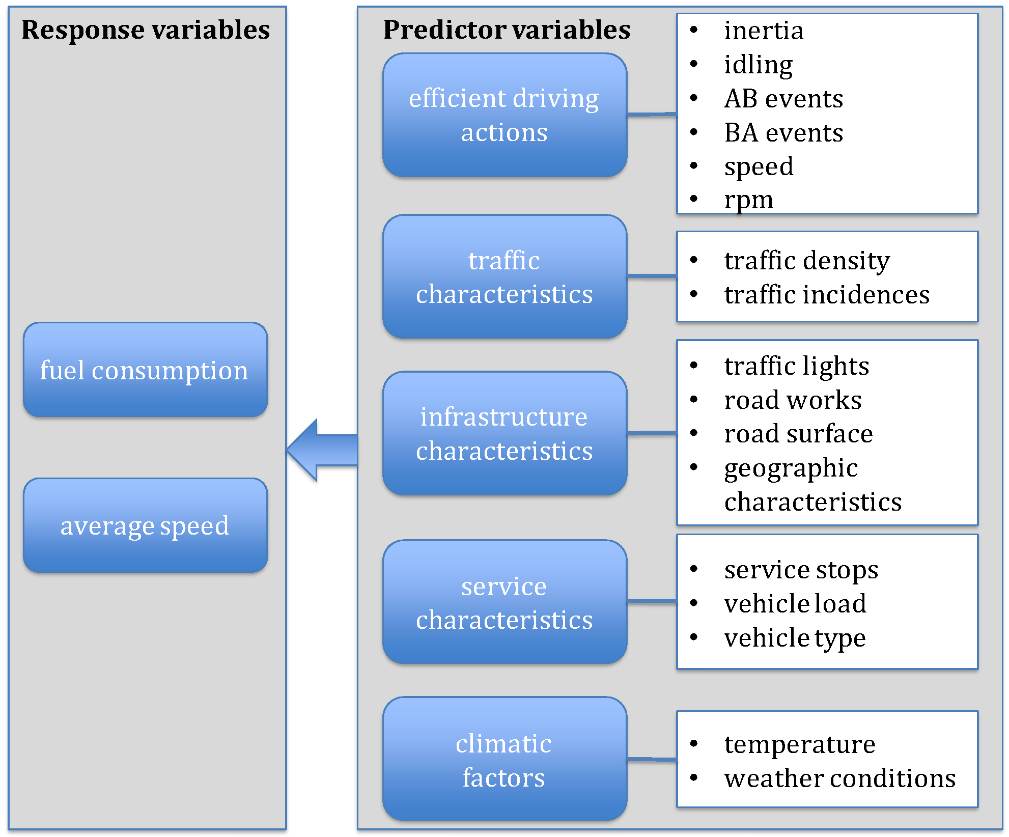
Figure 2.
Work methodology.

Figure 3.
Available parameters with external data integration. The variables included in the model are marked with ‘*’.
Figure 3.
Available parameters with external data integration. The variables included in the model are marked with ‘*’.
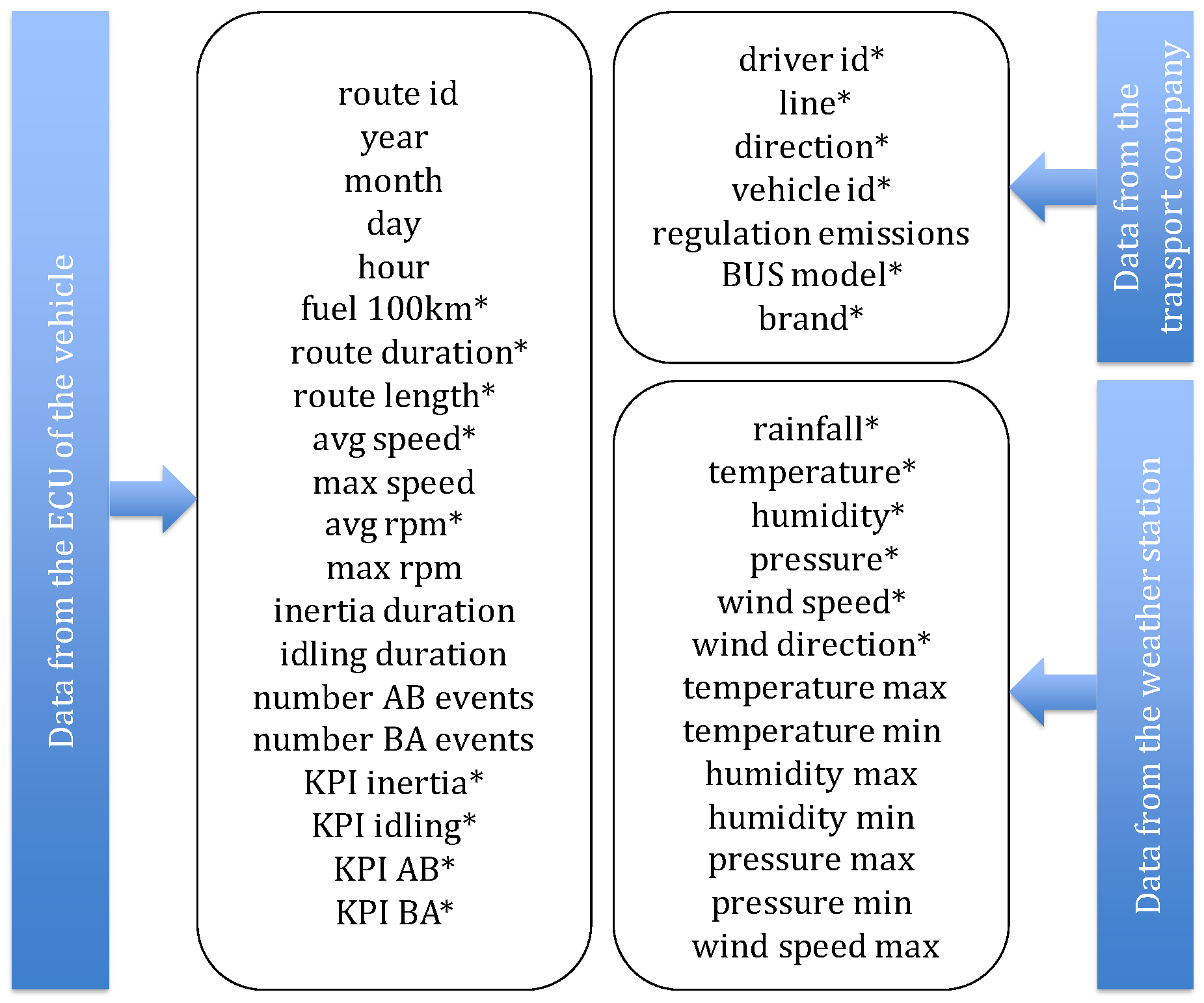
Figure 4.
Boxplot of fuel consumption vs. BUS model.

Figure 5.
Influence of driver and BUS Model on fuel consumption.
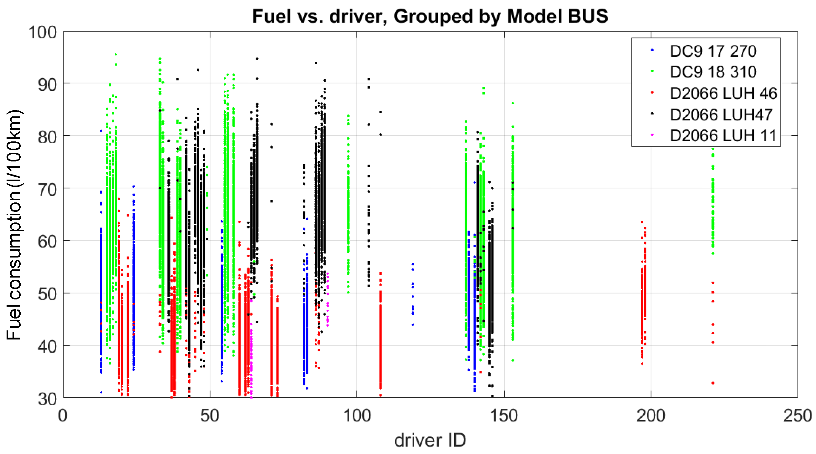
Figure 6.
Influence of driver for the bus #15 and route #12.

Figure 7.
Influence of the efficient patterns on fuel consumption. (a) Fuel consumption vs. inertia pattern; (b) Fuel consumption vs. idling pattern; (c) Fuel consumption vs. AB pattern; (d) Fuel consumption vs. BA pattern.
Figure 7.
Influence of the efficient patterns on fuel consumption. (a) Fuel consumption vs. inertia pattern; (b) Fuel consumption vs. idling pattern; (c) Fuel consumption vs. AB pattern; (d) Fuel consumption vs. BA pattern.
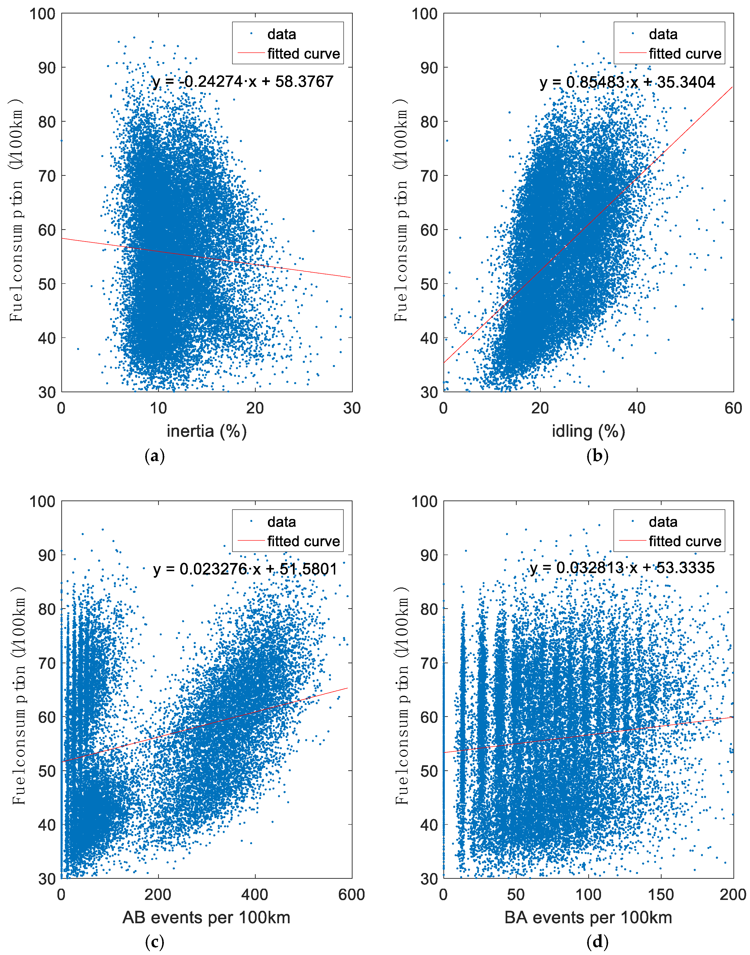
Figure 8.
Effect of the whole model on fuel consumption.

Figure 9.
Effect of the predictors on fuel consumption.

Figure 10.
Effect on changing inertia and idling for the evaluated buses. (a) Effect on changing inertia; (b) Effect on changing idling.
Figure 10.
Effect on changing inertia and idling for the evaluated buses. (a) Effect on changing inertia; (b) Effect on changing idling.

Figure 11.
Effect on changing AB and BA patterns for the evaluated buses. (a) Effect on changing AB pattern; (b) Effect on changing BA pattern.
Figure 11.
Effect on changing AB and BA patterns for the evaluated buses. (a) Effect on changing AB pattern; (b) Effect on changing BA pattern.
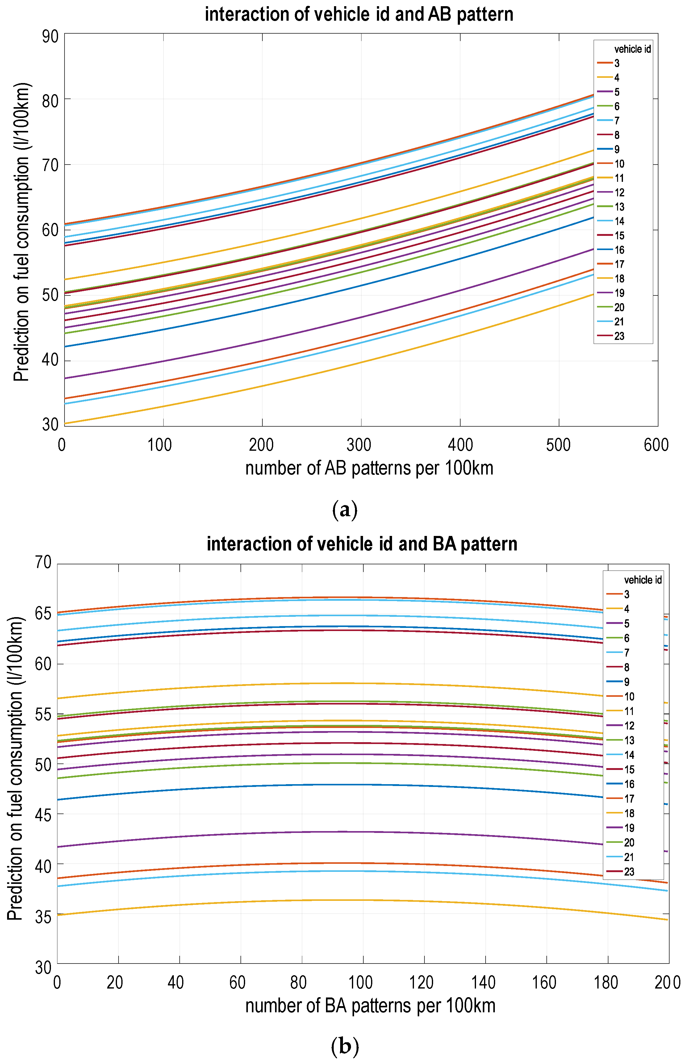
Table 1.
Description of the traces collected from the vehicle under test.
| Parameter | Description |
|---|---|
| Vehicle id | identifier of the vehicle associated with the collected data |
| Route id | identifier of the route |
| Distance | total distance of the vehicle in km |
| Timestamp | date and time of the day when the registered events have occurred, with the format YYYY-MM-dd hh:mm:ss.xxx |
| Speed | average speed of the vehicle in km/h |
| RPMs | average of RPMs (revolutions per minute) of the engine |
| Selected gear | current engaged gear |
| Acceleration | average acceleration of the vehicle in m/s2 |
| Accelerator pedal position | position of the accelerator pedal, measured in percentage |
| Brake switch | identifies whether the brake pedal is in use |
| Fuel consumption | instantaneous fuel consumption of the vehicle in l/h |
| Latitude | GPS latitude coordinate |
| Longitude | GPS longitude coordinate |
Table 2.
Summary of the efficiency patterns.
| Pattern | Conditions | KPI |
|---|---|---|
| Inertia | speed ≠ 0; fuel consumption = 0 or speed ≠ 0; gear ≠ 0; accelerator = 0 | time percentage in inertia in relation to the total duration of the route |
| AB | a > 0 → (t ≤ 2 s) → brakes = 1 or a > 0 → (t ≤ 2 s) → a ≤ −0.882 (m/s2) | number of AB pattern occurrences per 100 km |
| BA | a ≤ −0.882 (m/s2) → a < 0; v ≠ 0 → a > 0 | number of BA pattern occurrences per 100 km |
| Idling | v = 0 (t ≥ limits) | time percentage spent idling in relation to the total duration of the route |
Table 3.
VIF for the predictor variables.
| Variable Name | VIF |
|---|---|
| ‘route_duration’ | 10.137 |
| ‘route_length’ | 10.855 |
| ‘KPI_inertia’ | 2.365 |
| ‘KPI_idling’ | 4.503 |
| ‘KPI_AB’ | 6.759 |
| ‘KPI_BA’ | 1.982 |
| ‘avg_speed’ | 8.842 |
| ‘avg_rpm’ | 2.626 |
| ‘rainfall’ | 1.200 |
| ‘temperature’ | 1.662 |
| ‘humidity’ | 1.339 |
| ‘pressure’ | 1.645 |
| ‘wind_speed’ | 1.522 |
| ‘wind_direction’ | 1.033 |
Table 4.
VIF for the selected predictor variables.
| Variable Name | VIF |
|---|---|
| ‘KPI_inertia’ | 2.340 |
| ‘KPI_idling’ | 3.926 |
| ‘KPI_AB’ | 6.529 |
| ‘KPI_BA’ | 1.971 |
| ‘avg_speed’ | 3.043 |
| ‘avg_rpm’ | 2.596 |
| ‘rainfall’ | 1.199 |
| ‘temperature’ | 1.661 |
| ‘humidity’ | 1.337 |
| ‘pressure’ | 1.645 |
| ‘wind_speed’ | 1.522 |
| ‘wind_direction’ | 1.032 |
Table 5.
Continuous and dummy variables in the model.
| Coefficient ID | Variable Name | Description | Type |
|---|---|---|---|
| β0 | constant | Constant (intercept) term | Continuous |
| β1–β57 | driver_id_i | 1 if driver ID = i, 0 otherwise | Dummy |
| β58–β76 | vehicle_id_j | 1 if vehicle ID = j, 0 otherwise | Dummy |
| β77–β80 | BUSmodel_k | 1 if BUSmodel is k, 0 otherwise | Dummy |
| β81 | brand_MAN | 1 if brand is MAN, 0 otherwise | Dummy |
| β82–β90 | line_l | 1 if line is l, 0 otherwise | Dummy |
| β91–β105 | direction_m | 1 if direction is m, 0 otherwise | Dummy |
| β106 | KPI_inertia | Measured inertia in % | Continuous |
| β107 | KPI_idling | Measured idling in % | Continuous |
| β108 | KPI_AB | Measured AB pattern in events/100 km | Continuous |
| β109 | KPI_BA | Measured BA pattern in events/100 km | Continuous |
| β110 | avg_speed | Average speed of the route in km/h | Continuous |
| β111 | avg_rpm | Average rpm of the route in rpm | Continuous |
| β112 | rainfall | Rainfall in the day of the route in mm | Continuous |
| β113 | temperature | Average temperature in °C | Continuous |
| β114 | humidity | Average humidity day in % | Continuous |
| β115 | pressure | Average pressure in hPa | Continuous |
| β116 | wind_speed | Average wind speed in m/s | Continuous |
| β117 | wind_direction | Average wind direction in degrees | Continuous |
Table 6.
Quantitative savings in fuel consumption by improving driving from 25% to 75%.
| Variables | Quartile 25 (Inefficient) | Median | Quartile 75 (Efficient) |
|---|---|---|---|
| Driver ID | 63 | ||
| Vehicle ID | 13 | ||
| Line ID | 15 | ||
| Direction ID | 9 | ||
| Avg_speed (km/h) | 23.05 | ||
| Avg_rpm (rpm) | 903.45 | ||
| Rainfall (mm) | 13.50 | ||
| Temperature (°C) | 13.05 | ||
| Humidity (%) | 70.50 | ||
| Pressure (hPa) | 1014.75 | ||
| Wind_speed (m/s) | 1.40 | ||
| KPI_inertia (%) | 9.2 | 10.8 | 13.3 |
| KPI_idling (%) | 29.1 | 22.3 | 18.3 |
| KPI_AB (events/100 km) | 328.1 | 85.7 | 32.9 |
| KPI_BA (events/100 km) | 96.3 | 66.3 | 38.5 |
| Fuel consumption (L/100 km) | 61.79 | 50.22 | 45.79 |
© 2017 by the authors. Licensee MDPI, Basel, Switzerland. This article is an open access article distributed under the terms and conditions of the Creative Commons Attribution (CC BY) license (http://creativecommons.org/licenses/by/4.0/).
Share and Cite
MDPI and ACS Style
Garcia, R.; Diaz, G.; Pañeda, X.G.; Tuero, A.G.; Pozueco, L.; Melendi, D.; Sanchez, J.A.; Corcoba, V.; Pañeda, A.G. Impact of Efficient Driving in Professional Bus Fleets. Energies 2017, 10, 2060. https://doi.org/10.3390/en10122060
AMA Style
Garcia R, Diaz G, Pañeda XG, Tuero AG, Pozueco L, Melendi D, Sanchez JA, Corcoba V, Pañeda AG. Impact of Efficient Driving in Professional Bus Fleets. Energies. 2017; 10(12):2060. https://doi.org/10.3390/en10122060
Chicago/Turabian StyleGarcia, Roberto, Gabriel Diaz, Xabiel G. Pañeda, Alejandro G. Tuero, Laura Pozueco, David Melendi, Jose A. Sanchez, Victor Corcoba, and Alejandro G. Pañeda. 2017. "Impact of Efficient Driving in Professional Bus Fleets" Energies 10, no. 12: 2060. https://doi.org/10.3390/en10122060
Note that from the first issue of 2016, this journal uses article numbers instead of page numbers. See further details here.