Two-Sided Tacit Collusion: Another Step towards the Role of Demand-Side

Abstract

In the context of agent-based simulation framework of collusion, this paper seeks for two-sided tacit collusion among supply-side and demand-side participants in a constrained network and impacts of this collusion on the market outcomes. Tacit collusion frequently occurs in electricity markets due to strategic behavior of market participants arose from daily repetition of energy auctions. To attain detailed analysis of tacit collusion, state-action-reward-state-action (SARSA) learning algorithm and the standard Boltzmann exploration strategy based on the Q-value are used to model market participants’ behavior. A model is presented that integrates exploration and exploitation into a single framework, with the purpose of tuning exploration in the algorithm. In order to appraise the feasibility of collusion, a theoretical study on a three-node power system with three scenarios is depicted considering three Gencos and two Discos which proves the formation of two-sided tacit collusion between Genco and Disco. Simulation results show different collusive strategies of participants and how parameters of the algorithm impact on simulation outcomes. It is also shown that congestion on transmission line has a significant influence on behavior of market participants.

1. Introduction

The electricity market is a double-sided auction in which supply-side and demand-side participants can freely trade energy in different time horizons. Under this regime, electricity trading is usually conducted in various forms: a real-time (RT) market, a day-ahead (DA) market, an hour-ahead market, and a long-term contract market [1]. Restructuring of the electricity markets has led to the emergence of collusion, which frequently occurs due to the behavior of participants and their learning from the environment. Generally, collusion is defined as agreements or intrigues between sellers to raise or fix prices and to lower output in order to increase profits [2]. Previous studies have drawn attention to collusion in which only supply-side participants are concerned. In [3], an agent-based simulation has been employed to demonstrate that generators can learn from repetition of auction to withhold capacity based on publicly available (LMP) information. A novel method for tacit collusion ex ante detection has been presented in [4], which compared the outcome of tacit collusion with Nash equilibrium using a distributed optimization concept. In [5], tacit collusion is analyzed in repeated uniform price auctions where firms with symmetric and capacity-constrained characteristics compete in an oligopoly market. The analysis sets a target to study the sustainability of collusion under two pricing rules, i.e., uniform and discriminatory. In these studies, firms learn to engage in collusion with the primary focus on supply-side participants. Thus the literature on the effect of an active demand side participant on tacit collusion is sparse. The aim of this work is to prove the possibility of collusion between supply-side and demand-side participants by which the utilities of the participants will be analyzed.

The complexities of electricity market operation and daily repetition of electricity auctions have driven new trends in modeling methods of power market participants’ behavior [6]. One of the most attractive new methods, which is widely used to investigate various economic systems, is agent-based modeling, which provides insight into the behaviors of participants in a complex environment [7]. An agent-based model is a computational model that simulates interactions of adaptive agents to assess their effects on market outcome [8]. Each agent is able to interact with an environment, sense a state, and take actions to attain a goal that increases its respective rewards. An agent-based model was used in [9] for analyzing the German electricity market and the effects of the strategic behavior of market participants, as well as the limitations that congestion in the grid might impose on market outcomes. The result indicates substantial interdependence between the effects of strategic behavior in the market and congestion in the German grid. In [10], an agent-based model has been used to demonstrate the impact of consumers’ price elasticity on electricity market performance. Results show a reduction in congestion costs and market power of Gencos by demand-side bidding and consumers’ awareness of demand responsiveness.

Reinforcement learning is a type of agent-based learning that permits agents to automatically ascertain the effective behavior and learn their behavior using interaction with the environment in order to maximize the reward [11]. Q-learning is one of the most notable reinforcement learning algorithms, and has been comprehensively used in the modeling of participants’ behavior [12,13]. It is a simple, model-free method for agents to learn how to behave optimally and evolve their strategic behavior. The other reinforcement learning algorithm, SARSA, which uses five events (state-action-reward-state-action) to update the Q-values, is an on-policy reinforcement learning algorithm [14]. Learning in SARSA depends upon the current policy that is conducted by the agent.

Modeling the power market as a repeated game of supply and demand side, this paper seeks to apply the SARSA algorithm to the decision-making of a Genco and a Disco, which use the repetition of the game to form a two-sided implicit collusion and increase their payoffs. Instead of using a greedy policy, a model that allows tuning continual exploration in an optimal way is used to integrate exploration and exploitation in a common framework, as presented in [15]. It first defines the degree of exploration of a state as the entropy of probability distribution to quantify exploration in order to select an acceptable action in that state. Then, to balance exploration and exploitation in a single framework, a global optimization problem is considered: searching to discover the exploration strategy that maximizes the expected cumulated profit fixing exploration degrees in that state. In order to select actions, it employs the Boltzmann strategy based on the Q-value.

The aim of this paper is to investigate the behavior of players in a constrained network and the development of two-sided tacit collusion between a Genco and a Disco whose behaviors are modeled through the SARSA learning algorithm. This paper is organized as follows: Section 2 presents the DA electricity market structure. Section 3 describes the SARSA learning algorithm and a model for tuning exploration based on Q-values. Theoretical background is used to illustrate the possibility of collusion between a Genco and a Disco in Section 4. Simulation results are presented in Section 5 and, finally, Section 6 summarizes our main conclusions.

2. Electricity Market Structure

This paper investigates the behavior of Gencos and Discos in the DA electricity market, where seller and buyer agents engage in our simulation framework. Each agent is designed to be provided with learning capabilities. The design of learning capabilities depends upon the environment and the goals that the agent is trying to achieve. In the DA auction with a daily merit order settlement mechanism, n Gencos (i = 1,…,n) submit their offers P_i,t and b_i,t, and similarly, m Discos submit their bids q_k,t and b_k,t (k = 1,…,m) for 24 periods (t = 1,…,24).

2.1. Supply-Side in DA Market

The i-th Genco with net capacity P_i,t^max at the t-th period submits P_i,t (P_i,t ≤ P_i,t^max). The offering amount is determined by P_i,t = φ_i,t P_i,t^max, where φ_i,t (0 ≤ φ_i,t ≤ 1) is a decision parameter to express the proportion of the offering amount to the net capacity. Moreover, the price that a Genco offers is expressed by b_i,t = (MPC_i,t)/(1 − σ_i,t), which must be greater than or equal to the Genco’s marginal production cost, MPC_i,t and less than or equal to the market price cap. The difference between the mark-up of the offer price and the marginal cost is reflected in σ_i,t, which captures the strategic behavior of offering price.

2.2. Demand-Side in DA Market

The k-th Disco predicts electricity demand (q_k,t) on a delivery day using a forecasting method and also estimates a bidding price (b_k,t) through a function (F) of demand, b_k,t = F(q_k,t). Since the retail price (b_k^ret) is fixed, it is not considered a crucial variable. Determination of the bidding amount of the Disco comprises a two-level decision-making process. First, the Disco selects interruptible load (IL) contract d^IL_k,t (d^IL_k,t ≤ d_IL^max), which is executed by d^IL_k,t = μ_k,t d_IL^max in which μ_k,t (0 ≤ μ_k,t ≤ 1) and d_IL^max are decision parameters chosen in accordance with the Disco’s portfolio and the maximum available interruptible load contracts, respectively. Secondly, the Disco determines the bidding amount of demand, q°_k,t (q°_k,t = q_k,t − d^IL_k,t) .The bidding price of the Disco is determined by b_k,t = η_k,t b_k^ret, in which η_k,t (0 ≤ η_k,t ≤ 1) is a decision parameter to express the reduced offering price to the fixed retail price.

2.3. ISO Market Clearing Problem

In the wholesale power market, whose structure is based on the DA electricity market, independent system operator ISO uses a uniform (or single) price clearing auction, in which Gencos place offers with an independent market administrator for a particular time period. Similarly, each Disco sets a bidding quantity and price for demand. After submitting the offers and bids of the Gencos and Discos, ISO clears the market based on the merit order settlement mechanism and computes the quantities, a real power allocation to the i-th Genco (P_i,t^acc), a demand allocation to the k-th Disco (q_k,t^acc) and Locational Marginal Prices, LMP_k, by solving the optimal power flow (OPF) equations considering transmission line limits and ramp constraints of Gencos.

2.4. The Disco’s Cost Minimization Problem

The total DA cost of the Disco’s system operation is considered the cost function of the Disco. The goal of the Disco is to select the optimal energy bid parameters (μ_k,t, q°_k,t) in order to minimize the following cost function in the DA market:

$${U_k}^{Disco}={\displaystyle \sum _{t=1}^{24}}\{{\mathrm{b}}_{\mathrm{t}}{q_{k,t}}^{acc}+{\mu }_{k,t}{d_{IL}}^{max}{C}_{IL}+{b_t}^{ext}({q°}_{k,t}-{q_{k,t}}^{acc})\}.$$

(1)

Three parts of cost function are the cost of purchasing power from the market, cost of utilizing IL contract and the cost of out of equilibrium demand (q°_k,t − q_k,t ^acc). If the bidding amount lies beyond the equilibrium point, Disco will be obliged to purchase (q°_k,t − q_k,t ^acc) at an external price.

2.5. Genco’s Profit Maximization Problem

The goal of each Genco is to select the optimal energy offer parameters (φ_i,t, λ_i,t) in order to maximize the profit function in the DA market:

$${U_i}^{Genco}={\displaystyle \sum _{t=1}^{24}}\{b_t-MP{C}_{i,t}\}{P_{i,t}}^{acc}.$$

(2)

The ramp constraints should be respected for generating power at every hour, as given in the following [8]:

$${\phi }_{i,t+1}{P_{i,t+1}}^{max}-{\phi }_{i,t}{P_{i,t}}^{max}\le RU{P}_i$$

(3)

$${\phi }_{i,t}{P_{i,t}}^{max}-{\phi }_{i,t+1}{P_{i,t+1}}^{max}\le RD{P}_i.$$

(4)

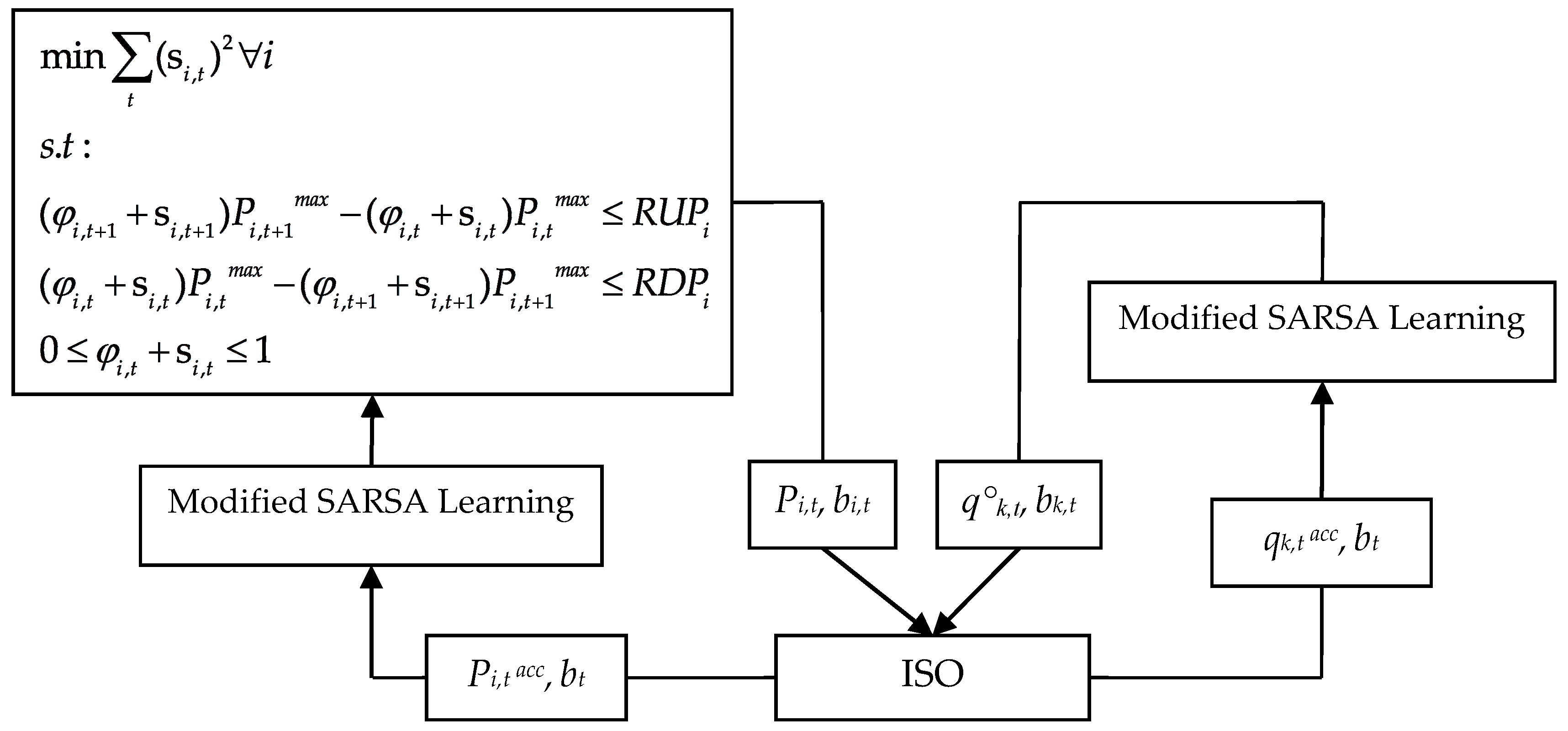
Figure 1 shows the market coordination mechanism and offering and bidding process of Gencos and Discos in a single scheme. As described before, Gencos and Discos submit their offers and bids to the ISO and then he clears the market. After that, Gencos and Discos using modified SARSA learningalgorithm try to improve the offering and bidding parameters. Note that each Genco looks for feasible decision parameter (φ_i,t) by minimizing slack variable (s_i,t) [8,16]. Section 3 describes the SARSA learning process and modifies it using the Boltzmann exploration strategy based on the Q-value, by which Gencos and Discos can “learn” through the repetition of the DA energy auction to choose the parameters of their energy offers and bids, based only on market clearing price (b_t).

3. Learning Process

3.1. SARSA Learning Algorithm

The SARSA algorithm [14], which considers both exploration and an unknown environment, approximates the Q-learning values by averaging out empirically both the uncertainty about the action to choose and the uncertainty about the next state [15]. An experience in SARSA is of the form [s, a, r, s’, a’], which makes up a transition from state-action pair, (s, a), to state-action pair, (s’, a’), with reward r. This leads to a new experience to update action value, Q(s, a), whose general form is expressed by the following scheme:

$$Q\left(s_t,a_t\right)\leftarrow Q\left(s_t,a_t\right)+{\alpha }_t[r_t+\gamma Q\left(s_{t+1},a_{t+1}\right)-Q\left(s_t,a_t\right)],$$

(5)

where Q(s_t, a_t) is the expected value function that agent g will take by performing the given action a_t in state s_t. α_t is learning rate in the range of [0, 1). γ (0 ≤ γ ≤ 1) is discount factor and r_t is the reward value received as the result of taking action a_t in state s_t.

The discount factor γ reflects that future value matters less than the present value. Agent chooses a_t to maximize the expected discounted reward:

$$E_t=R(t+1)+\gamma R(t+2)+{\gamma }^{2}R(t+3)+\dots ={\displaystyle \sum _{t=1}^{\infty }}{\gamma }^{t-1}R(t+1).$$

(6)

If γ is close to 0, the agent is “myopic,” which indicates that it tries to maximize immediate rewards; thus the object of the agent is to maximize only reward R(t + 1); on the other hand, when γ is close to 1, the agent is farsighted and takes into account the future rewards more firmly.

Q-learning learns the value of the optimal policy, independent of the current policy as long as it explores enough. In fact, the last action chosen has a vital role in updating the Q-value and the agent with pure exploitation about its information chooses the next action, whereas SARSA explores actions in order to optimize the value of a policy. For this reason, introducing a model allowing continual exploration in an optimal way to make tradeoffs between exploration and exploitation is the major issue. This paper uses a model presented in [15] to control the balance between exploration and exploitation in a common framework, where exploration is defined as the association of a probability distribution to the set of available action-state pairs. The (Shannon) entropy is utilized to quantify the degree of exploration in a state as the entropy of this probability distribution. Furthermore, it uses the standard Boltzmann exploration strategy based on the Q-value. As shown in simulation experiments of [15], “the Boltzmann method outperforms the ε-greedy method”.

3.2. The Standard Boltzmann Exploration Strategy Based on the Q-Value

Let us assume that agent g at time t chooses a control action a in state s_t = s (there are n states in total) with probability distribution π_s(a). With executing the chosen action a, it receives immediate reward r(s, a), and jump to the next state s_t+1 = s’. The policy ∏ ≡ {π_s(a), s = 1,2,…,n} defines for each state s a probability distribution π on the set A(s) of available actions in that state. Then the probability distribution π_s(a) for choosing control action a in state s (which is a multinomial logistic function) is:

$${\pi }_s\left(a\right)=\frac{\exp [{\theta }_{s}Q\left(s,a\right)]}{{\displaystyle \sum _{j\in A\left(s\right)}}\exp [{\theta }_{s}Q\left(s,j\right)]},$$

(7)

which corresponds to Boltzmann strategy including the Q-value. θ_s ≥ 0 is the inverse of the temperature parameter. The degree of exploration E_s at each state s considering the probability distribution π_s(a) is defined as in [15]:

$$E_s=-{\displaystyle \sum _{a\in A\left(s\right)}}{\pi }_s\left(a\right)log{\pi }_s\left(a\right).$$

(8)

This is known as the Shannon entropy of the probability distribution of choosing control actions in state s [17,18]. Note that θ_s is a function of predefined E_s, i.e., θ_s(E_s). Therefore, first, θ_s is computed through Equation (8) and then π_s(a) is updated. In the case of no uncertainty, E_s is equal to zero, which corresponds to the one-step Q-learning algorithm. From the other point of view, when there is maximum uncertainty, E_s is equal to log(n_s), where n_s is the number of available actions in state s, therefore, π_s(a) = 1/n_s (a uniform distribution). On the one hand, when θ_s = 0, the probability distribution changes to random probability distribution and π_s(a) = 1/n_s, which corresponds to maximum degree of exploration (log(n_s)) for all states. On the other hand, E_s = 0 corresponds to pure exploitation; therefore, the algorithm selects a strategy based purely on the current value of the state-action pairs. Consequently, an optimal exploration that maximizes the expected payoff is determined by the selection of E_s in the interval 0 < E_s < log(n_s). Moreover, the definition of the exploration rate E_r^s at state s is the proportion of degree of exploration to the maximum degree for that state:

$${E_r}^s=E_s/log(n_s),$$

(9)

where E_r^s takes its values in the interval [0, 1] and for optimal exploration in the interval (0,1).

Based on the model described above, the SARSA learning algorithm can be modified by Algorithm 1. In the next section, a three-node system is considered to prove the possibility of tacit collusion between Genco and Disco.

Algorithm 1: Modified SARSA algorithm: executed by all Gencos and Discos

Initialize Q(s, a), $\forall s\in S,a\in A_g$, arbitrarily and $0<{E_r}^s<1$ Repeat (for each episode): (a) Initialize s (b) Repeat (for each step of episode): Calculate Es by: $$E_s={E_r}^{s}log\left(n_s\right)$$ Estimate θs using (8). Update probability distribution for state s as (7). Choose an action using probability distribution, receive immediate reward r and jump to the next state s’ Compute the expected Q-value: $$Q\left(s,a\right)\leftarrow Q\left(s,a\right)+\alpha [r+\gamma {\displaystyle \sum _{a^{\prime }\in A\left(s^{\prime }\right)}}{\pi }_{s^{\prime }}\left(a^{\prime }\right)Q(s^{\prime },a^{\prime })-Q(s,a)]$$ s ← s´, a ← a´; until s is terminal.

4. The Theoretical Background of Tacit Collusion between a Genco and a Disco

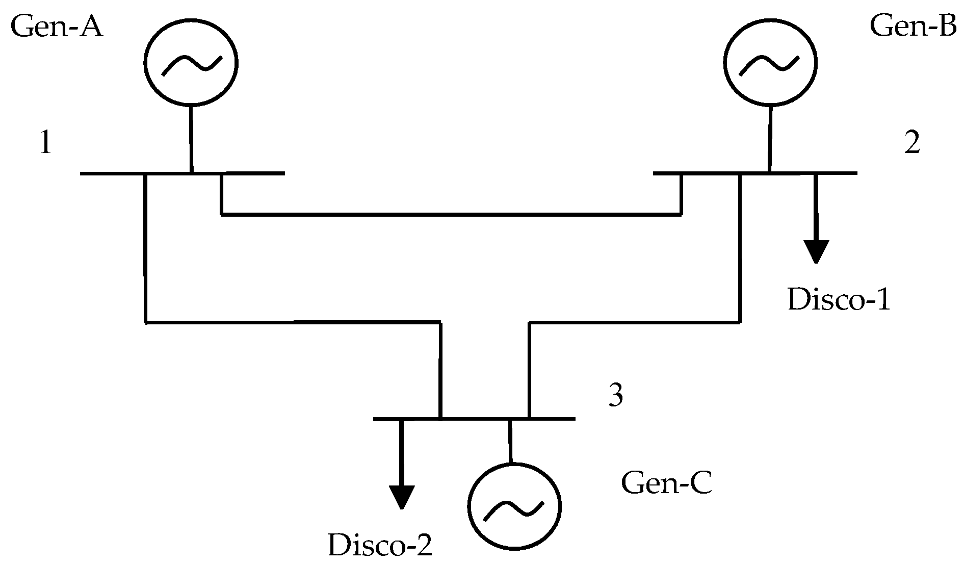
A simple, three-node system, presented in Figure 2, is used in order to prove that collusion between a Genco and a Disco is feasible. Three Gencos and two Discos, each with different sizes, and generation technology portfolios, are considered as market players that can improve their utility function through modified SARSA algorithm. Information on Gencos (net capacity and marginal cost) and transmission lines data (reactance and capacity) are shown in

Table 1. Generation data of Gencos (capacity, marginal cost).

Genco	Capacity (MW)	Marginal Cost ($/MWh)
Gen-A	200	6
Gen-B	200	10
Gen-C	200	8

and

Table 2. Transmission lines data (reactance, capacity).

Line No.	From Bus	To Bus	X (pu)	Flow Limit (MW)
1	1	2	0.2	100
2	1	3	0.2	200
3	2	3	0.1	200

, respectively. Detailed information on Discos, possible interruptible loads contracts, and retail price are also shown in

Table 3. Demand side information (b_k^ret, IL).

Disco	bkret ($/MWh)	qILmax (pu)	CIL ($/MWh)
1	11	0.3	2
2	10	0.2	2

. Furthermore, each Disco’s demand characteristics for two consecutive trading periods are presented in

Table 4. Disco’s demand in two consecutive hours.

Disco	Load(MW)
	First Hour Second Hour
1	100	120
2	100	120

.

In order to examine the effect of collusion on market outcomes, three scenarios are considered:

• Scenario A: Gen-A strategically offers in the first hour in order to withhold capacity and try to maximize its profit using modified SARSA learning.
• Scenario B: Gen-A strategically offers in both the first and second hours in order to raise its selling price when no collusion occurs.
• Scenario C: Gen-A withholds capacity in the first hour, while Gen-A and Disco-1 develop some kind of cooperation through the learning procedure in the second hour.

4.1. Scenario A: The Exercise of Market Power in the First Hour

Each Genco tries to maximize its objective function by selecting the optimal bidding strategy. In this scenario, we suppose that all Gencos are capable of learning, while Discos are not able to learn, which indicates that they behave as passive participants. If Gen-A strategically acts in order to maximize its profit by withholding capacity, it prevents the transmission line congestion and makes profit from this strategic behavior. In other words, when the generator agent of Node-1 offers below the threshold of 200 MW, it leaves the transmission line uncongested, therefore increasing its selling price to LMP of Node-3, which results in an increase in profit. In spite of that, if Gen-A offers 200 MW, the clearing price of Node-1 will be $6.64/MWh, while if it offers 199 MW, since there is no congestion, all Gencos are paid at the same system-wide market clearing price (MCP) ($8/MWh). As expected, by offering below 200 MW, Gen-A’s utility increases from $128 to $398. It is interesting to note that, although the generator agent of Node-1 does not have any information about the transmission limit, he can learn to withhold capacity and maximize his profit through learning.

4.2. Scenario B: The Exercise of Market Power in the First Hour and No Collusion in the Second Hour

In this scenario, we suppose that all Gencos are able to learn in both hours, while Discos are not capable of learning. Similar to the previous scenario, Gen-A has a learning capability by which it withholds capacity in the first hour, provided that he offers 199 MW to maximize his profit. Due to the network demand changes in the second hour in comparison to the first hour, as well as ramp-rate constraint, Gen-A cannot prevent network congestion. Therefore, the LMP at each node is equal to the marginal cost of the local generator and Gen-A does not make profit from the energy market, while the ISO collects congestion rent.

4.3. Scenario C: The Exercise of Market Power in the First Hour and the Emergence of Cooperation between a Genco and a Disco in the Second Hour

In this scenario, all Gencos and Discos are able to learn. Like the previous scenario, in the first hour, Gen-A tries to maximize its own earnings by offering strategically. Due to demand changes in comparison with the previous hour and ramp-rate constraint, Gen-A cannot exercise market power in the second hour and increase the price of Node-1, even if he offers 199 MW. On the other hand, congestion in the transmission line increases the price of Node-2, whose LMP is higher when the network is congested than when there is no congestion. To put it more simply, the reason for the higher price is transmission line congestion, which motivates Disco-1 to lower its load in order to reduce its total energy cost. It is certainly correct that when Disco-1 interrupts 20 MW of its load and simultaneously Gen-A offers 199 MW, there is no congestion in the transmission line and all Gencos are paid at the system-wide MCP ($8/MWh). Therefore, on the one hand, developing a tacit collusion between Gen-A and Disco-1 increases the price of Node-1 from $6/MWh to $8/MWh and, on the other hand, it decreases the LMP of Node-2 from $9/MWh to $8/MWh. In conclusion, it can be said that the result of this scenario denotes the emergence of an implicit cooperation, where Genco and Disco try to change the price and increase their utility, even though there is no communication between them.

Comparing the utility of Gen-A in Scenarios B and C, it can be concluded that Gen-A earns $398 in Scenario B, while its profit reaches $796 in Scenario C. This indicates that cooperation between Gen-A and Disco-1 significantly increases Gen-A’s profit. On the other hand, if Disco-1 interrupts its load and cooperates with Gen-A (Scenario C), managing to prevent the transmission line congestion, its utility will increase to $560, while if there is no cooperation between the Genco and the Disco (Scenario B), Disco-1’s utility will be $540. Given this, it can be concluded that collusion is profitable for both a Genco and a Disco in the second hour and it is more likely to occur.

5. Simulation Results

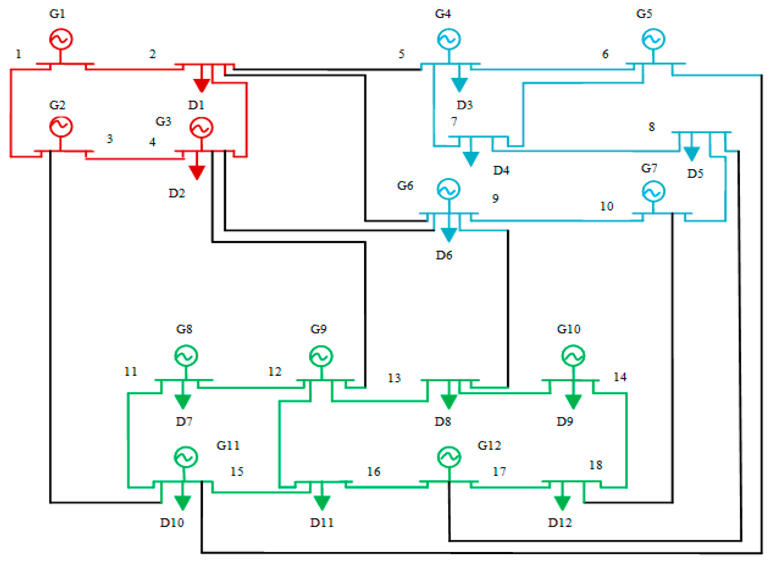
In this section, in order to examine the feasibility of the simulation framework, an 18-bus network, as shown in Figure 3, is used in which generation and demand sides portfolios have been allocated G1 to G12 and D1 to D12, respectively. Characteristics of Gencos, Discos, and transmission lines are given in

Table A1. Generation side data in an 18-bus network.

Genco	Marginal Cost ($/MWh)	Capacity (MW)
G1	15	1100
G2	21	1000
G3	24	900
G4	27	1500
G5	29	1000
G6	25	1100
G7	26	1200
G8	25	1000
G9	24	1300
G10	29	1300
G11	30	1200
G12	25	1100

,

Table A2. Demand side data in an 18-bus network.

Disco	Load (MW)	Retail Price ($/MWh)	CIL ($/MWh)
D1	1000	27	10
D2	800	29	10
D3	1000	30	10
D4	800	31	10
D5	900	33	10
D6	1000	32	10
D7	800	29	10
D8	700	30	10
D9	900	30	10
D10	1000	29	10
D11	800	29	10
D12	800	28	10

and

Table A3. Transmission line data.

Line No.	From Bus	To Bus	R(pu)	X(pu)	Flow Limit (MW)
1	1	2	0.005	0.15	500
2	1	3	0.01	0.1	600
3	2	4	0.01	0.1	500
4	2	5	0.01	0.1	500
5	2	9	0.005	0.15	700
6	3	4	0.005	0.15	400
7	3	15	0.02	0.1	700
8	4	9	0.02	0.1	600
9	4	12	0.005	0.15	400
10	5	6	0.02	0.1	700
11	5	7	0.005	0.1	600
12	6	7	0.005	0.15	400
13	6	15	0.005	0.15	500
14	7	8	0.01	0.1	500
15	8	10	0.01	0.1	600
16	8	17	0.02	0.1	400
17	9	10	0.005	0.15	400
18	9	13	0.01	0.1	600
19	10	18	0.01	0.1	600
20	11	12	0.01	0.1	700
21	11	15	0.02	0.1	500
22	12	13	0.02	0.1	500
23	12	16	0.005	0.1	500
24	13	14	0.005	0.15	600
25	14	18	0.005	0.15	600
26	15	16	0.01	0.15	500
27	16	17	0.01	0.1	400
28	17	18	0.01	0.1	500

in Appendix A. The network is divided into three zones specified by red, blue, and green. It is assumed that market participants can implicitly collude with each other in order to improve their utility functions. If G1 colludes with D3, it gains more profit than with the full capacity bidding strategy. G1 can collude with D3 directly or indirectly; in comparison to the direct method, the indirect method is more profitable, implying that G1 tries to collude with D3 using one of the two following methods:

(1)

in the first instance, collusion with D1, then collusion with D3;

(2)

in the first instance, collusion with D2, then collusion with D3.

Although collusion with D1 has more profit than collusion with D2, choosing the second method leads to higher aggregated profit than the first. If G1 is myopic, it chooses the first method, while foresight preference leads to choosing the second method.

To achieve tacit collusion, the parameters of the algorithm need to be set. The primary parameter that should be set is the exploration rate (E_r^s). With a low exploration rate close to 0%, the algorithm finds the strategy that has the maximum profit and, therefore, direct collusion with D3 is chosen. In order to attain collusion with D1 or D2, which contain less profit than collusion with D3, the exploration rate should be high. If the exploration rate is high, e.g., 90%, the algorithm chooses actions that lead to less profit than direct collusion. Under these conditions, the γ parameter (the discount factor) specifies that collusion with D1 or D2 is performed. With low amounts of γ close to 0, implying that myopic preference governs G1, the algorithm chooses the action that has more immediate profit, and collusion with D1 is more likely to occur while with discount factor close to 1, implying that foresight preference governs G1, the action with high long-term profit is chosen, and collusion with D2 will be performed.

Consider the case of G1, which wants to maximize its profit by implicit collusion with D3; it can implement this directly or indirectly. As discussed above, direct collusion does not depend on the discount factor, while indirect collusion with different discount factors leads to different results. In order to investigate the performance of G1 under different operational strategies in indirect collusion, two cases are examined:

✓

Case A: myopic preference of G1, which indicates that the discount factor is low (close to 0). In this case, G1 chooses actions that influence only the immediate rewards, not future rewards as well, so it maximizes (6) by separately maximizing each immediate reward.

✓

Case B: foresight preference of G1, which means the discount factor is high (close to 1). With a high discount factor, G1 will propagate its further rewards through the time.

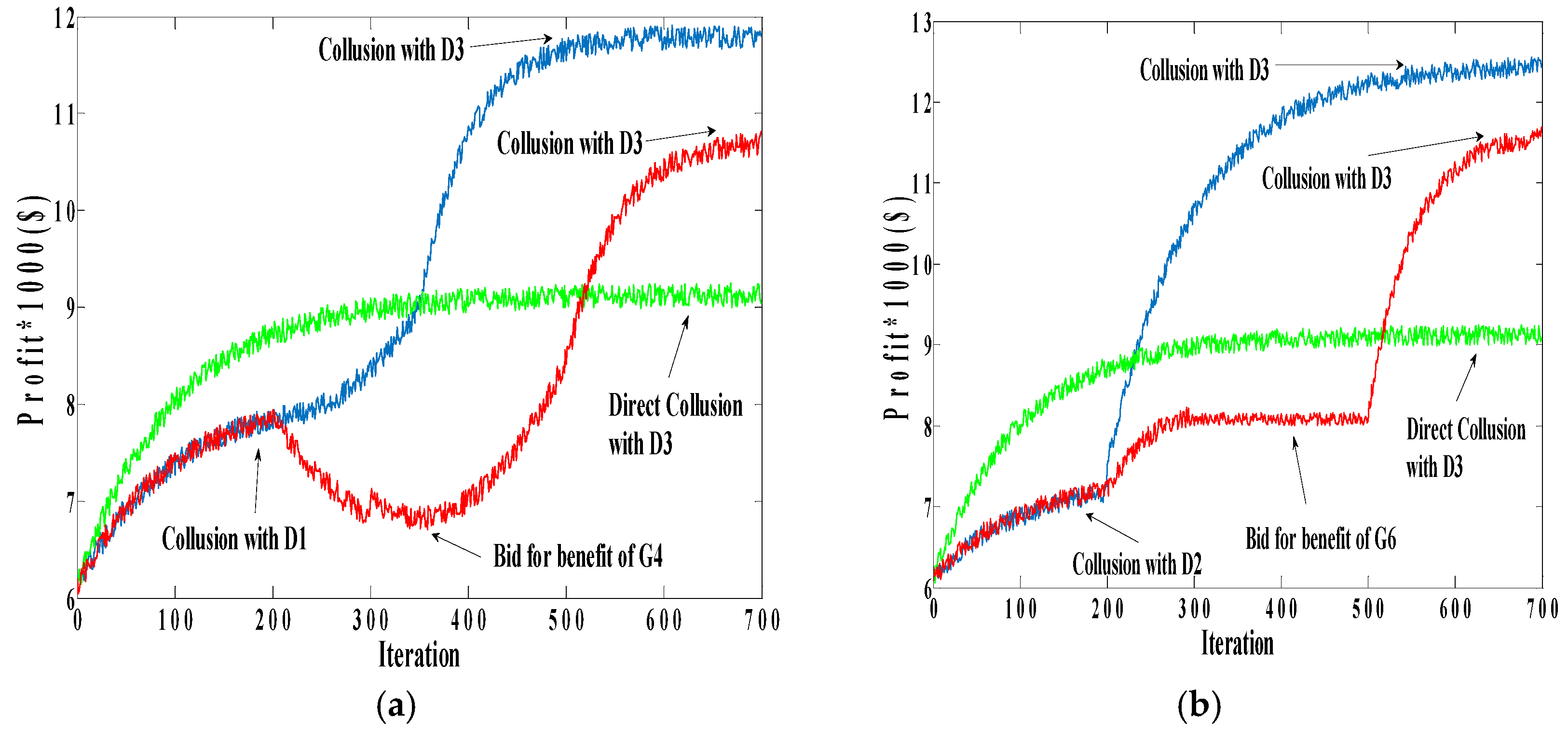
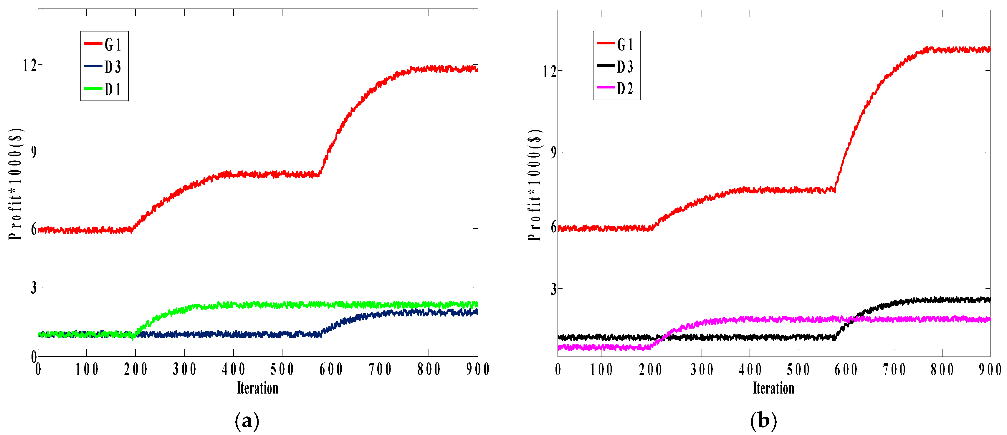
Figure 4 shows the profit functions of G1 in different conditions as per Case A and Case B, where final convergence of profit functions was obtained after almost 700 iterations. Based on Figure 4a, if G1 directly colludes with D3, it experiences an upward trend in its utility and earns $9100, while in indirect collusion, for which the profit is higher due to the low discount factor, G1 first colludes with D1 and earns $7700, then, if D1 remains loyal, G1 can collude with D3 and earns $11,850. In comparison, if D1 does not remain loyal, the profit of G1 experiences a downward trend, indicating that G1 has to bid for benefit of G4 to guarantee the loyalty of D1. Under these circumstances, the selling price and quantity of G4 increase and, on the other hand, the price of the node that D1 has been located on it decreases, which convinces D1 to remain loyal. Given the loyalty of D1, G1 eventually earns $10,700, which is more profit than from the direct collusion with D3. Figure 4b shows the utility functions of G1 in different conditions, as per Case B. As can be seen in this figure, G1 first colludes with D2 and earns $7200, then, if D2 remains loyal, G1 can collude with D3 and earns $12,400; otherwise, G1 has to bid for the benefit of G6 to maintain D2’s loyalty because this strategy decreases the price of the node that D2 has been located on it. As a consequence, although G1 earns less payoff when it colludes with D2, its final payoff in this case is more than with indirect collusion as in Case A.

Comparison of the profits of the two cases in indirect collusion with profit of direct collusion explains an important point: although some strategies have lower profit than other strategies, implementation of these strategies predisposes the players to execute strategies that will yield more profits in the long term.

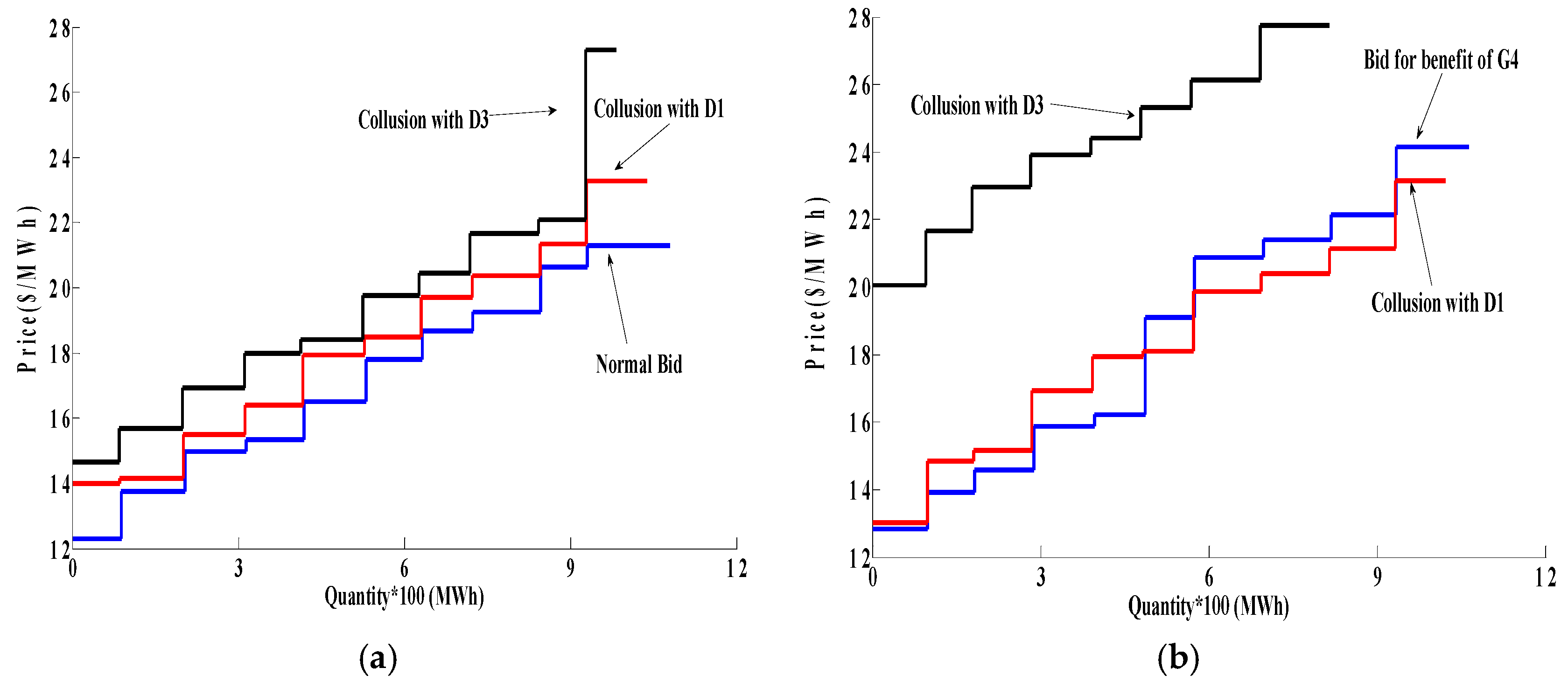
Figure 5 shows the bidding decisions of G1 in Case A. As shown in Figure 5a, G1 can learn to collude with D1 and increase its own selling price if it withholds capacity and bids 1060 MW. On the other hand, from Figure 6a, it can be seen that D1 lowers 40 MW of its demand and bids 960 MW. This strategy raises the selling price of G1 from $20.5/MWh to $22.3/MWh and, conversely, decreases the buying price of D1 from $26/MWh to $24/MWh. After that, if D1 remains loyal, collusion with D3 is possible by bidding 1000 MW and, at the same time, based on Figure 6b, D3 lowers 60 MW of its load by bidding 940 MW. The result of this strategy is a higher price for G1 ($26.8/MWh) and a lowered price for D3 (from $29 /MWh to $27/MWh). If D1 does not remain loyal, conditions change and thus G1 has to change its strategy and bid for the benefit of G4 (Figure 5b), which significantly decreases the selling quantity of G1 (850 MW) and consequently leads to lower profit in comparison to collusion with D1. After bidding to keep D1 loyal, G1 bids 820 MW, which indicates that it withholds 30 MW of its capacity and, on the other hand, D3 interrupts 30 MW of its load to clearing prices of nodes that G1 and D3 have been located on to attain $28.04/MWh and $27.4/MWh, respectively. 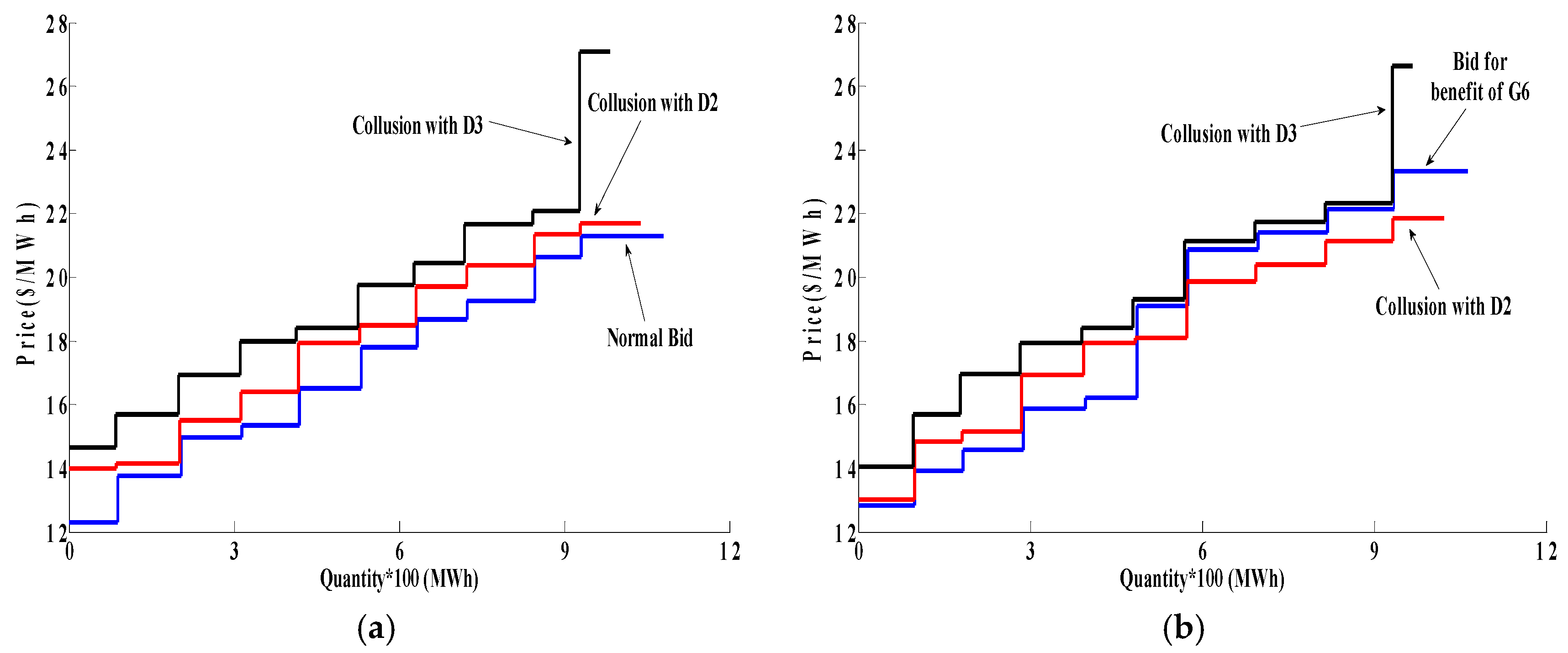Figure 7 shows bidding strategies of G1 in Case B. In the same way as in Figure 5, G1 increases its selling price by colluding with D2 instead of D1. Then, for loyalty of D2, he should bid for the benefit of G6, which makes possible the implementation of collusion with D3. From Figure 7a, it can be seen that G1 withholds 40 MW of its capacity by bidding 1060 MW to collude with D2 and raises the price to $21.8/MWh and, on the other hand, as shown in Figure 8, D2 simultaneously lowers 40 MW of its demand to decrease its buying price from $28/MWh to about $26/MWh. Afterward, G1 bids 1000 MW in order to collude with D3 and increase its selling price to $27.4/MWh, which is possible when D2 remains loyal. With the defection of D2, G1 can keep D2 loyal providing it changes its own bidding strategy and bids 1030 MW and finally colludes with D3 by bidding 1000 MW, i.e., by withholding 30 MW of its capacity (Figure 7b). As can be seen in Figure 6b, there is no difference for D3 when G1 colludes with either D1 or D2, whereas the loyalty or defection of D1 or D2 can change the LMP of the node that D3 has been located on.

Figure 9 shows profit functions of G1 and Discos in Case A and Case B. As expected, when G1 and D1 (D2) learn to collude with each other, their utilities are increased and both of them make a profit from this collusive behavior. After that, D1 (D2) keeps its strategy unchanged, which leads to a fixed amount of profit as before, while D3 experiences an upward trend in its profit, indicating that D3 has entered into the collusive strategy.

One essential question that should be answered is: why does G1 not collude with D1 (D2) and D3 simultaneously, in spite of the fact that finally collusion with D1 (D2) and D3 will occur? Or, perhaps it would be better to say, why does G1 collude with D1 (D2) and D3 one after the other?

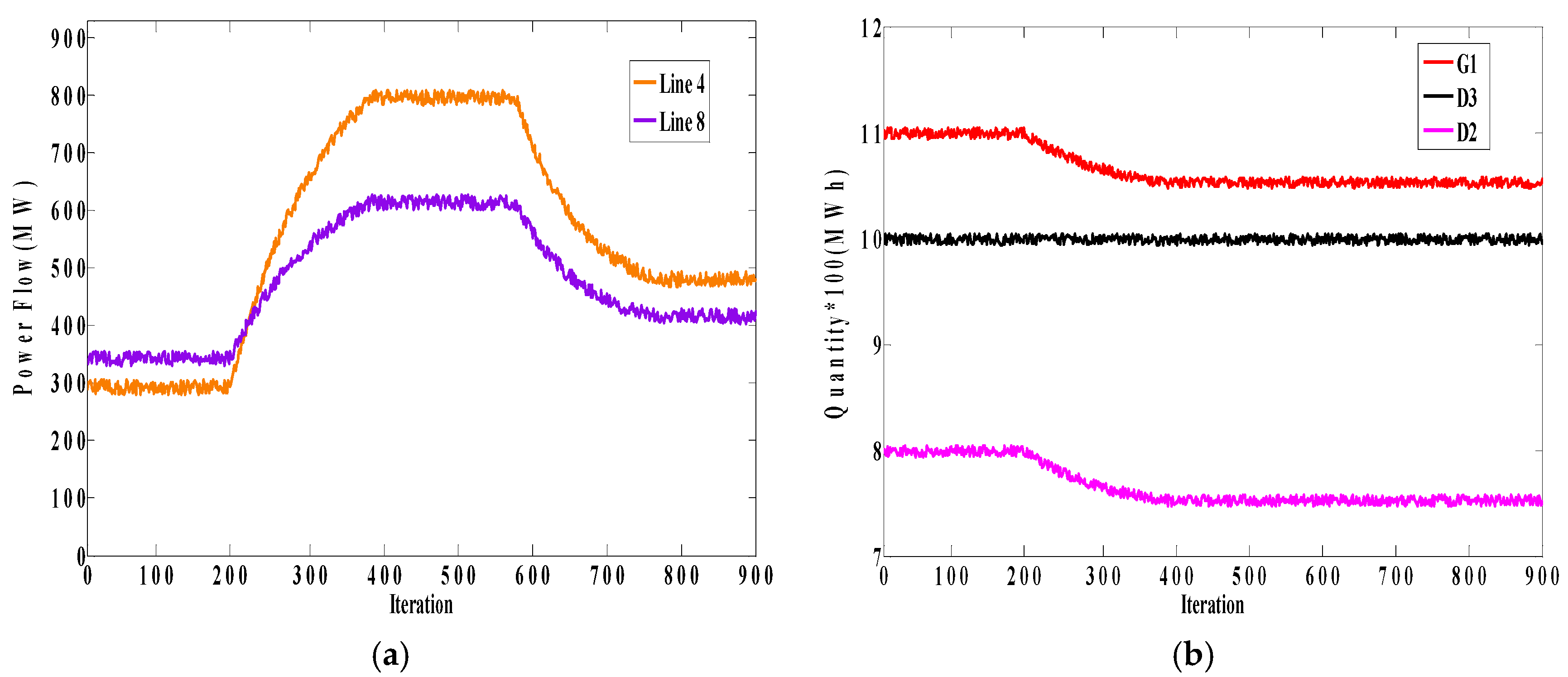
As discussed in Section 4, congestion on the transmission line has a significant influence on collusion and creates an incentive for Genco and Disco to tacitly collude. As stated before, the test system consists of three zones. G1, D1, and D2 are located in the first zone, while D3 is located in the second one. These two zones are connected through Lines 4, 5, and 8. In order to evaluate the effect of line congestion on the decision-making process of D3, we assess power flows of lines that are congested when G1 colludes with D1 (D2).

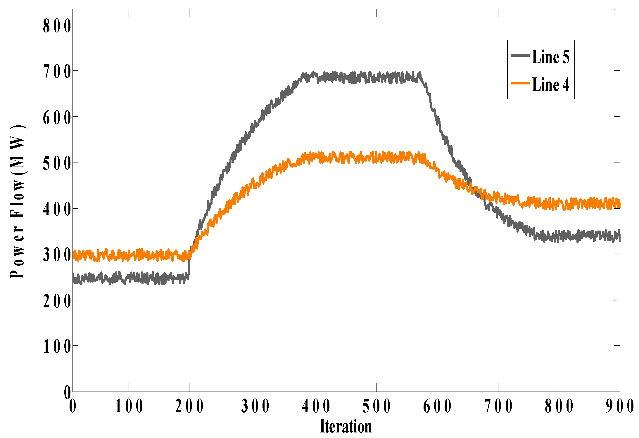
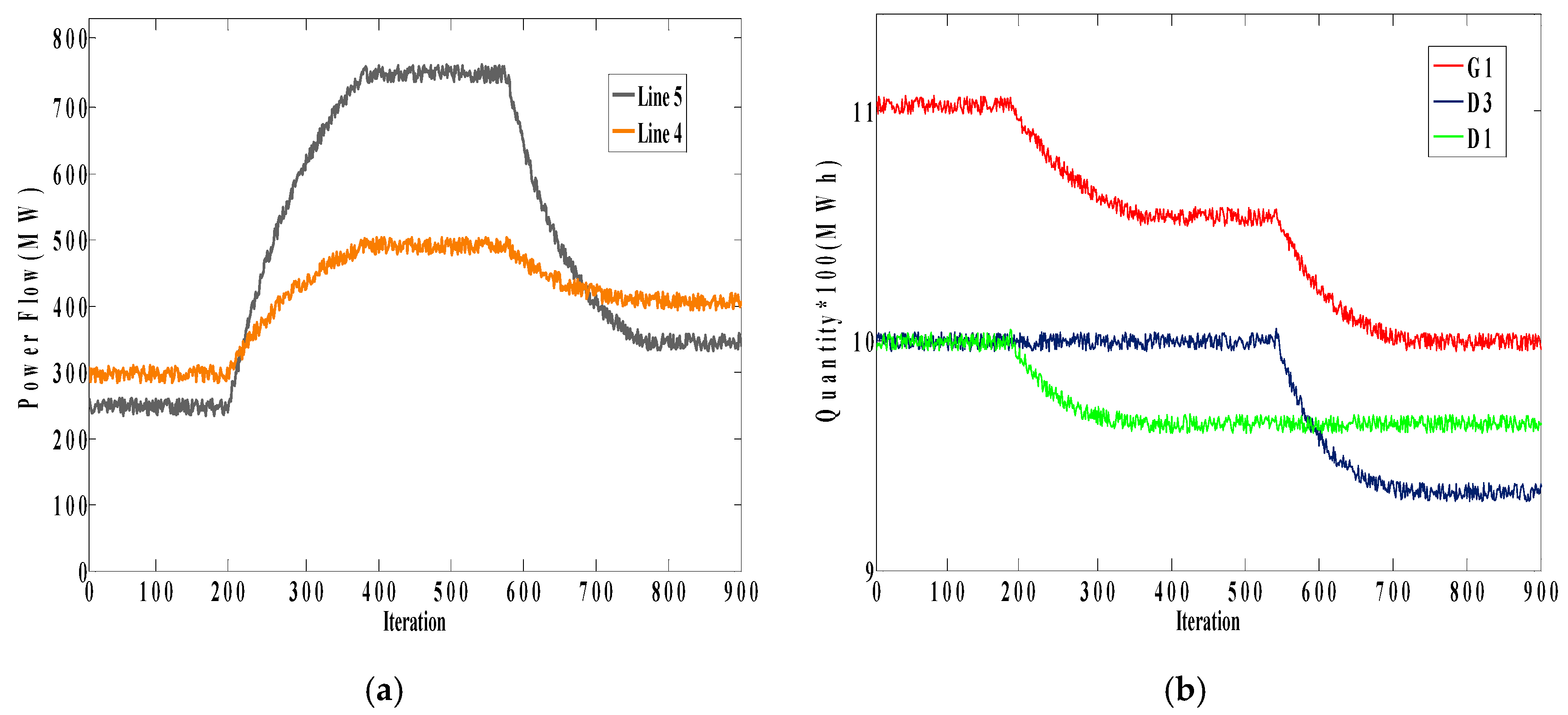
Figure 10 shows flows of Lines 4 and 5 in Case A. As can be seen, when G1 begin to collude with D1 (Iteration 200), the flows of these lines increase, and when these lines are congested, D3 enters into collusion with G1. To examine the behavior of D3, a two-step test is performed; in each step, we increase the limit of one line to be uncongested when G1 colludes with D1, while the other line limit remains unchanged.

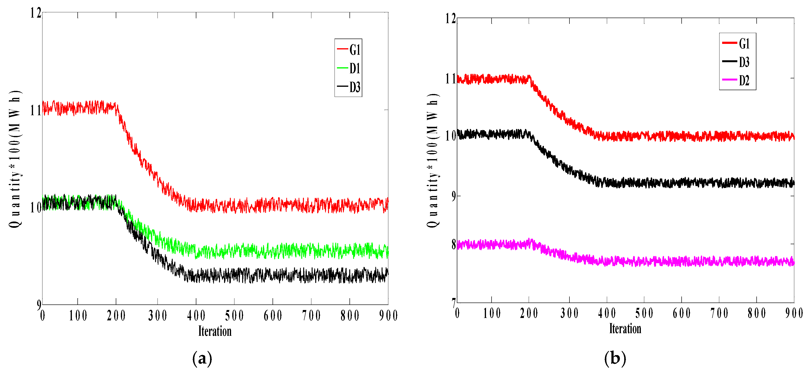
Step 1: f ^max (4) = 500 MW, f ^max (5) = 800 MW

Figure 11 shows flows of Lines 4 and 5 and behavior of players in this step. It can be seen from the figure that when Line 5 is uncongested, D3 still colludes with G1, which means that congestion on Line 5 does not have any influence on the behavior of D3.

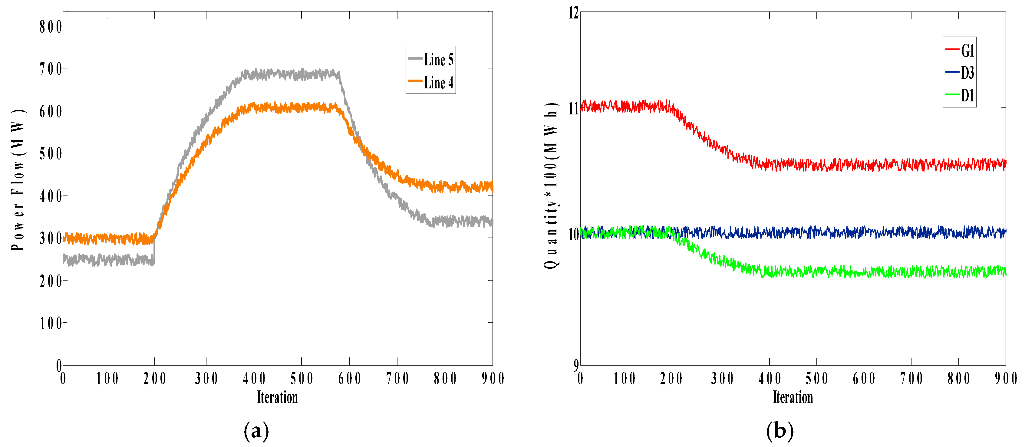
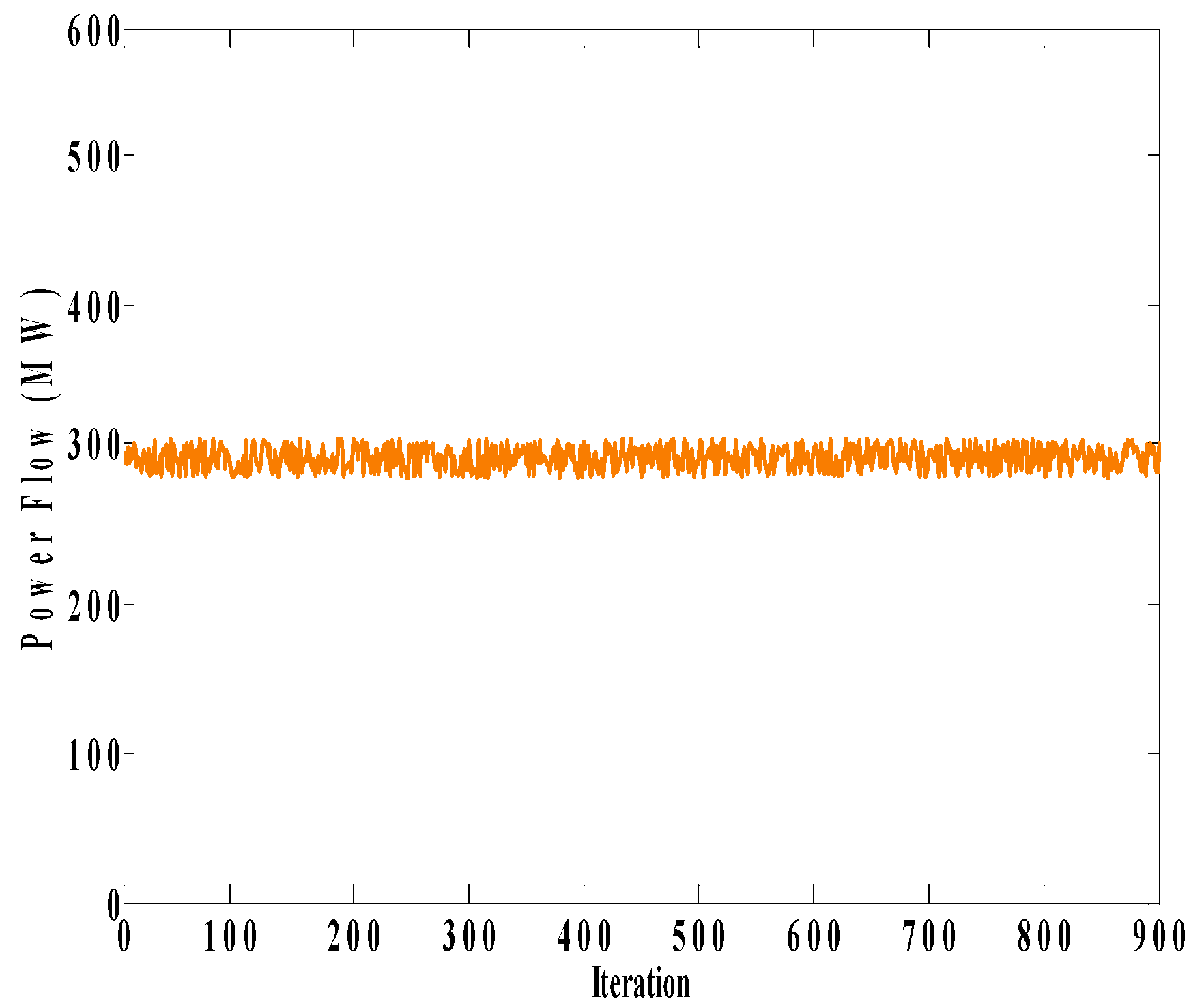
Step 2: f ^max (4) = 700 MW, f ^max (5) = 700 MW

Figure 12 shows the flows of Lines 4 and 5 and the behavior of players in this step. Unlike the previous step, when the limit of Line 4 increases, D3 does not enter into collusion with G1 and its strategy remains fixed. Therefore, it can be concluded that congestion on Line 4 has led to collusion of G1 with D3.

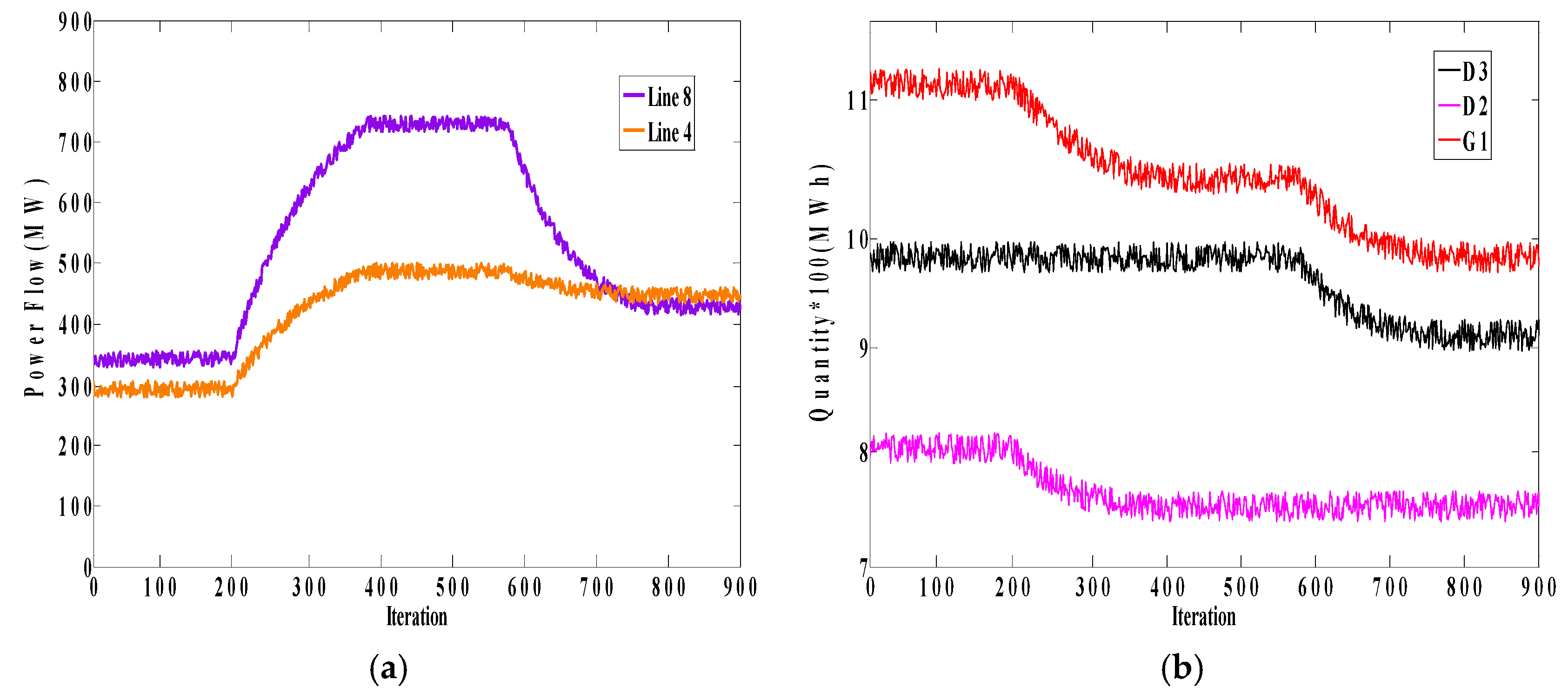
Figure 13 shows the flows of Lines 4 and 8 in Case B. As shown in this figure, when these lines are congested, D3 enters into collusion with G1. We also perform the two-step test for Case B.

Step 1: f ^max (4) = 500 MW, f ^max (8) = 800 MW

Figure 14 shows the flows of Lines 4 and 8 and the behavior of players in this step. As can be seen, when the limit of Line 8 increases, the behavior of D3 does not change, which means that the decision-making process of D3 does not depend upon the congestion of Line 8.

Step 2: f ^max (4) = 900 MW, f ^max (8) = 600 MW

Figure 15 shows the flows of Lines 4 and 8 and the behavior of players in this step. Based on these figures, when Line 4 is not congested, D3 does not enter into collusion with G1 anymore and its bidding strategy remains fixed. Consequently, it can be concluded that, as in Step 2 in Case A, congestion on Line 4 has a direct influence on collusive behavior between G1 and D3, such that without congestion this collusion does not form.

Now, we set the limit of Line 4 on the level that flows through this line before forming collusion of G1 with D1 (D2) in order to evaluate the behavior of D3. Figure 16 and Figure 17 show the power flow of Line 4 and the behavior of the market players in the two cases, respectively. As can be seen from Figure 16, Line 4 is always congested. As expected, according to Figure 17a, due to congestion on Line 4, G1, D1, and D3 decrease their bidding quantities at the same time until collusive behavior is reached. The behavior of players in Case B is much the same as that of the players in Case A. The only difference is the bidding quantity of G2, which is lower than the bidding quantity of D1. The figures concluded that the learning capability of D3 depends on the congestion on Line 4 and whenever Line 4 is congested, D3 can learn to collude with G1 and make profit in this way.

In this paper, market outcome expects tacit collusion among generation and demand side under particular circumstances. It is interesting to see how the set of constraints, i.e., the ramp rate of the generation side and the congestion of the network, lead the generation side to collude with the demand side. This adds more detail about the rationale behind this behavior and the degree of generality of the proposed simulation framework.

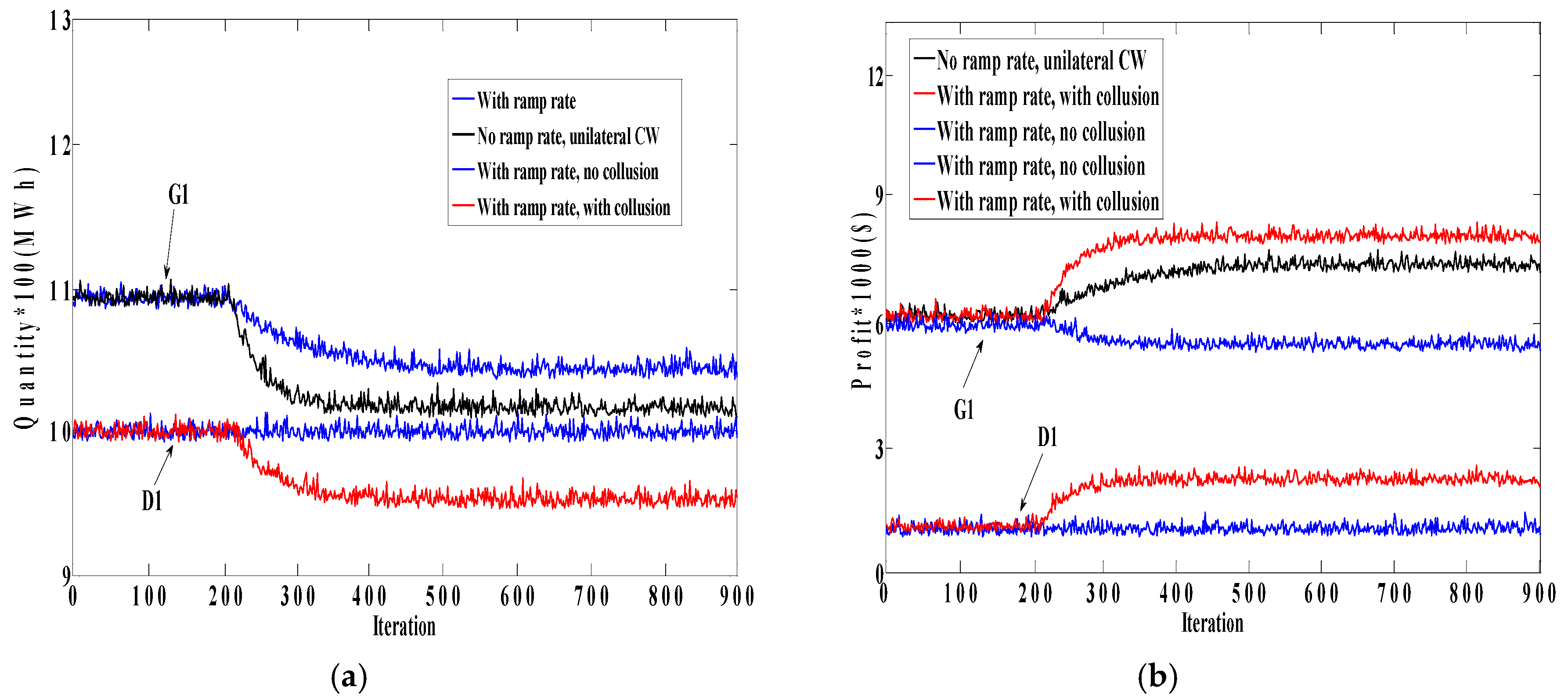
Figure 18 shows the quantity bidding of the Genco and the Disco and the corresponding profits in two conditions: with and without ramp rate constraint. As illustrated in the figures, when there is no ramp rate constraint, the Genco can unilaterally withhold 90 MW of its capacity in order to leave the transmission line uncongested, and thus it experiences an upward trend in its profit function. On the other hand, in the case of the ramp rate constraint, if the Genco unilaterally withholds capacity, it cannot prevent the transmission line congestion and raise its profit. As shown in the values with the tag of “With ramp rate, no collusion” in Figure 18b, due to a reduction in quantity of the Genco (from 1100 MW to 1060 MW) without any change in price, its profit tends to decrease. In this case, if the Disco lowers 40 MW of its demand in order to decrease its purchasing price, not only does it alleviate the ramp rate constraint of the Genco, but it also makes profit by preventing transmission line congestion. In other words, with the introduction of ramp rate constraint, the generation side needs the demand side to put effective collusion into practice, raising the price and utility.

6. Conclusions

This paper presented an analysis of the development of tacit collusion between a Genco and a Disco in a simulated constrained power market, where the power market operation was formulated as a repeated game. Gencos’ and Discos’ behaviors were modeled using the SARSA learning algorithm and a model was used to tune continual exploration and make the tradeoff between exploration and exploitation. To prove the possibility of tacit collusion between a Genco and a Disco, a market with three Gencos and two Discos in a simple three-node system was illustrated. Three scenarios are examined and it was shown that the development of this collusion increases their utilities.

In order to evaluate the feasibility of a simulation framework, a market with different sellers and buyers was simulated. Two case studies with different preferences were presented to examine how a Genco’s decision-making process is affected by different discount factors, where if the Genco is far-sighted, it can choose collusive strategies that have low short-term payoffs (collusion with D2) but the implication of these strategies causes a significant increase in the Genco’s payoff in the long term. It was shown that transmission line congestion has a direct impact on the implementation of collusive behavior and enables the Disco to learn to collude with the Genco.

Based on these observations, the authors have been conducting complementary studies dedicated to using regulatory intervention and tools to suppress the adverse effects of two-sided tacit collusion on market performance. Concentrating on regulatory tools of forward markets, the possibility assessment of two-sided collusion has to be broadened to include the impacts on the forward market. To be able to capture the forward market effects, the incorporation of a multi-settlement system, involving the DA operation of this paper and an extra forward market mechanism is required.