2.1. Low-Dimensional Modeling
The anti-slug control-oriented low-dimensional model applied in this study is an extension of the pipeline-riser model developed in [
15]. The model is based on 4 Ordinary Difference Equations (ODEs) with nonlinear functions describing 4 state variables,
. The model is divided into two sections: the pipeline section, and the riser section. Hence, the states describe the masses of gas and liquid in both the pipeline and the riser, respectively. The four state equations of the model are based on the following mass balance equations:
Here
is the pipeline gas mass,
is pipeline liquid mass,
is the riser gas mass, and
is the riser liquid mass.
is the gas-liquid mass ratio out of the riser. The pipeline mass inflow of gas,
, and liquid,
, are assumed to be disturbances to the system, while the mass flow rates from the pipeline to the riser,
and
are described by virtual valve equations. The outlet mixture mass flow (
) is calculated based on a valve equation with the topside choke valve opening (
z) which also is a model input, see Equation (
5).
where
is the combined gas and liquid mass flow through a choke valve,
is the mixed density,
is the pressure after the valve,
is the pressure before the valve,
is a static function for the choke valve opening,
is the cross-section area,
n has a value of 1 for laminar flow and 2 for turbulent flow and
is a tuning parameter which is further explained in
Section 2.3. The mixed density is calculated as the combined gas and liquid masses over the volume:
The entire model is highly nonlinear as the valve equations, the friction and the are derived from several nonlinear equations.
In this study several modifications have been added to the model to improve the accuracy of the model. The adjustments are listed here:
Extending the static linear choke valve equation to an exponential relationship;
Including two different Darcy friction equations;
Introducing a new topside pressure to precisely model the topside friction; and
Addition of a new tuning parameter, , which is a liquid blowout correction factor.
The valve opening is changed from a static linear relationship, , to a static exponential relationship where which is obtained from the choke valve’s datasheet and experimental tests. The choke valve used in this work is a globe valve which is a preferred valve type in offshore installations. This adjustment gives a more accurate bifurcation point and choke-to-production rate relationship. Please notice that the relationship does not apply for , however this is outside the operational range (due to safety regulations with very small valve openings) and thus does not cause any model inaccuracy within the operational region.
Two different Darcy friction factors are applied in this model: One for the calculation of the friction loss in the pipeline and one for the friction loss in the riser. For the horizontal pipeline a friction factor,
, obtained from [
16] was used:
where
Here
is the mixed density in the pipeline,
is the superficial mixed flow velocity at the pipeline inlet,
is the Reynolds number of the fluid mixture in the pipeline,
is the pipeline diameter and
is the mixed viscosity in the pipeline.
is calculated as the sum of superficial gas and liquid velocities:
where
and
.
is calculated as:
where
is the gas-liquid mass ratio in the pipeline. The riser friction factor,
, was obtained from the Haaland equation [
17]:
where
is the roughness of the riser,
is the Reynolds number of the fluid mixture in the riser, and
is the diameter of the riser.
is obtained from a calculation similar to Equation (
8). Even though the fiction coefficients can be calculated in different ways, Equations (
7) and (
11) are applied, respectively, because the results were closer to the data from the testing facility.
A new topside pressure point upstream the choke valve (
) is being introduced for improving the accuracy of Equation (
5). This pressure is derived from the topside pressure (
) subtracted with the pressure generated by the topside pipeline friction (
), such that
. The topside valve equation now uses
instead
. The value of
will vary further from
the longer the topside choke valve is located from the riser top. The friction for
is calculated similar to the friction Equation (
11). Note that
is not considered a model output similar to
, but is used for improving the model accuracy for (another output)
.
2.2. Test Rig
The small-scale experiments in this study is carried out on pipeline-riser slug testing facility located at Aalborg University Esbjerg. The slug testing facility is an extension of the facility examined in [
11,
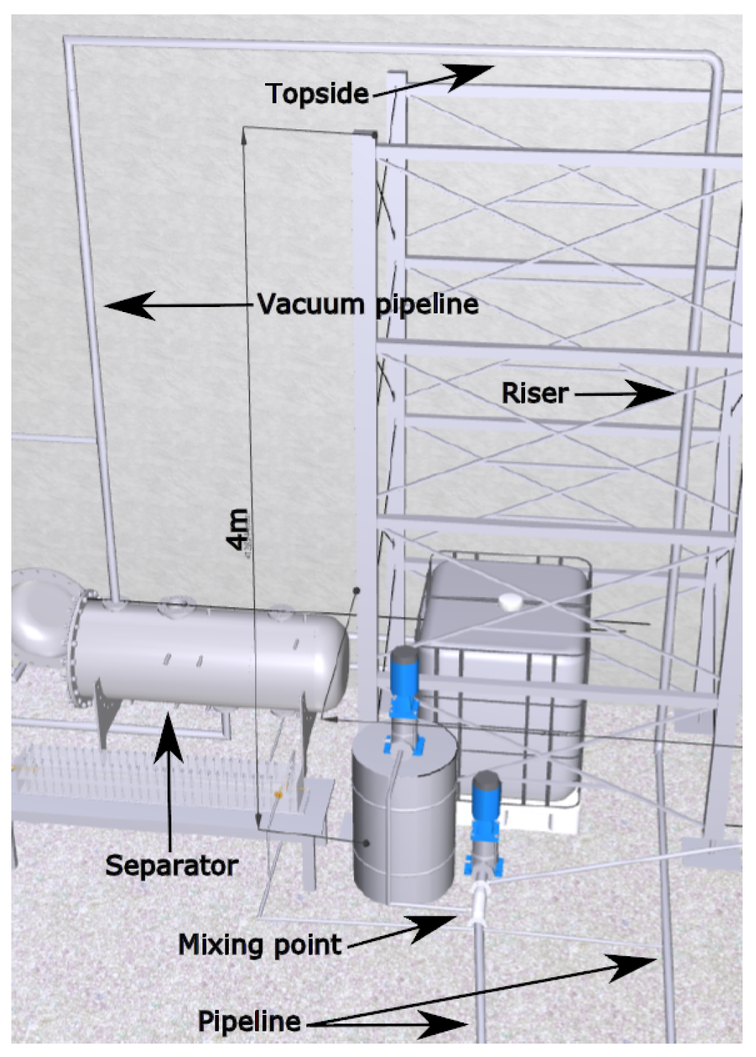
18]. The new testing facility can be observed in
Figure 1. The physical changes in the testing facility mainly consist of longer pipelines: 16 m horizontal pipeline, 4 m inclination pipeline, 4 m riser and 1.2 m topside pipeline from riser top to the topside choke valve. The outlet of the topside choke valve is connected to a vertical descending vacuum pipeline 3 m down to a 3-phase gravity separation, where the gas-liquid separation is carried out. The gravity separator is specially designed and currently has a 5 min separation buffer time (for the examined inflow conditions), however the weir level inside the separator can be adjusted in an offline manner if required for new testing conditions. The pipeline-riser dimensions can be found in
Table 1. The pressure and flow measurement uncertainties have been reduced by installing new equipment in a narrower range than in [
11,
18], such that the pressure measurement uncertainty now is 0.01 bar and the flow measurement uncertainty now is
kg/s. However, it has to be noted that the multi-phase flow transmitters are more uncertain the more gas is present in the pipeline, as they are measured by Coriolis flow meters. The software system is implemented in Simulink/MATLAB environment on a PC. For data acquisition an NI PCI-6229 DAQ-card is utilized and the central software system links the physical interface card through the Simulink Desktop Real-time (previously known as Real-time Windows Target) which guarantees Real-Time implementation.
For all the tests in this paper the inflow is constant (
kg/s and
kg/s), with the only exceptions of the input disturbances’ tests in
Section 5. The gas mass inflow is controlled by a bürkert MFC8626 solenoid valve after the compressor, and the product has a built-in PID mass flow controller for single-phase gas which has a fast tracking capability (within 5 s) without causing any visible overshooting. The liquid mass inflow is controlled by a centrifugal pump with measurement from an electromagnetic flow meter, where a PI controller is implemented, dedicated for obtaining a step response settling time under 10 s without any overshoot. The work in [
19] showed that both the gas and water inflow controllers have a fast bandwidth compared to dynamics of the entire system, hence these control loops do not have any significant unintended influence to the complete system’s behavior.
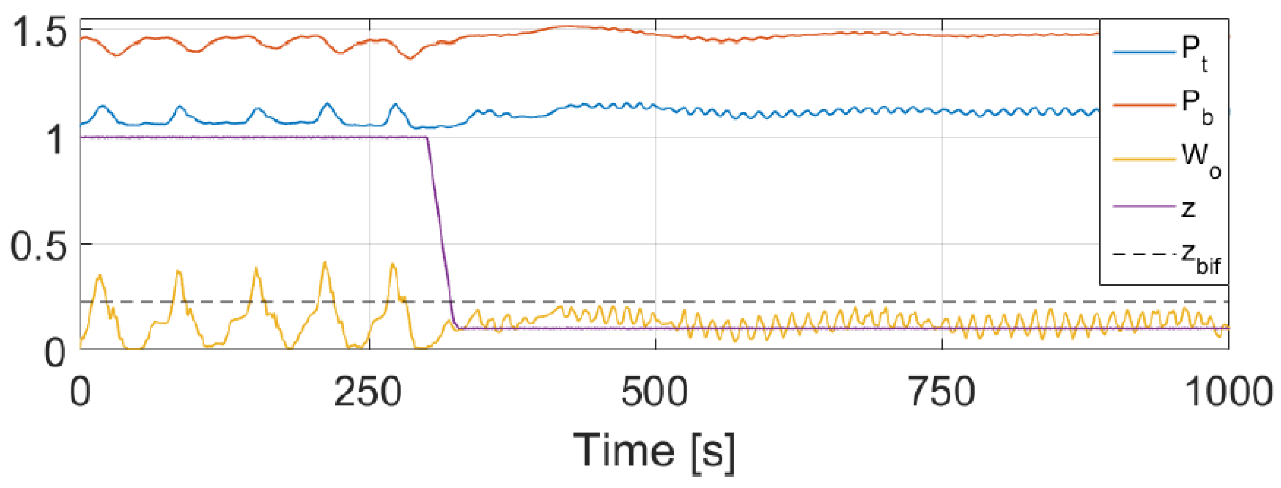
Figure 2 shows the step response of the slug testing facility where the valve goes from full open to 10% opening at 300 s. It is clear that the system initially is slugging before being stabilized as a consequence of the valve choking. One severe slug cycle lasts approximately 70 s. The open-loop bifurcation point (the changing from slug to steady flow) during these running conditions is at
valve opening. The high frequency oscillations at non-slug flow (after 300 s) exist due to the vacuum pipeline downstream the choke valve. The pipeline is not entirely vacuum and thus sucks the flow down the pipeline in a rapid cyclic manner.
2.3. Parameter Identification
A tuning guide is carried out in [
15] by isolating the dimensionless tuning parameters,
,
and
, in the valve equations (see Equation (
5)) with predefined operational points. Three correction factors were introduced:
,
and
. Each of these three new correction factors are dimensionless and should individually be close to a value of one. The relationship between the tuning parameters and the correction factors can be observed in Equations (
12)–(
14), where
,
,
and
is back calculated from the steady-state measured
,
,
,
and
.
is a non-slugging operational topside valve opening. Besides, a parameter correction factor was also considered for the steady-state level of liquid in the pipeline,
, however this correction factor performed the best for
.
In this study the model is further extended with a new tuning parameters,
, used to correct for how much of the liquid is flowing through the riser during the blowout stage of each slug cycle.
can be used to adjust for offsets in the pressure. In Equation (
15)
is included to calculate the liquid-volume-fraction out of the riser (
):
for
, where
is the area of liquid in riser lowpoint and
is the pipeline cross-section at riser lowpoint.
A collection of the identified model’s constants for the slug testing facility including the tuning parameters is listed in
Table 1. The overall accuracy of the model is significantly improved with the addition of the added
,
and
tuning parameters.
and
increases the simulating accuracy for the impact of valve manipulation in the region
, where the linear valve characteristic varies the most from the exponential characteristic. The inclusion of
both improves the simulation accuracy of the riser’s hydrostatic pressure offset, as well as the pressure and flow amplitudes of the severe slugs.
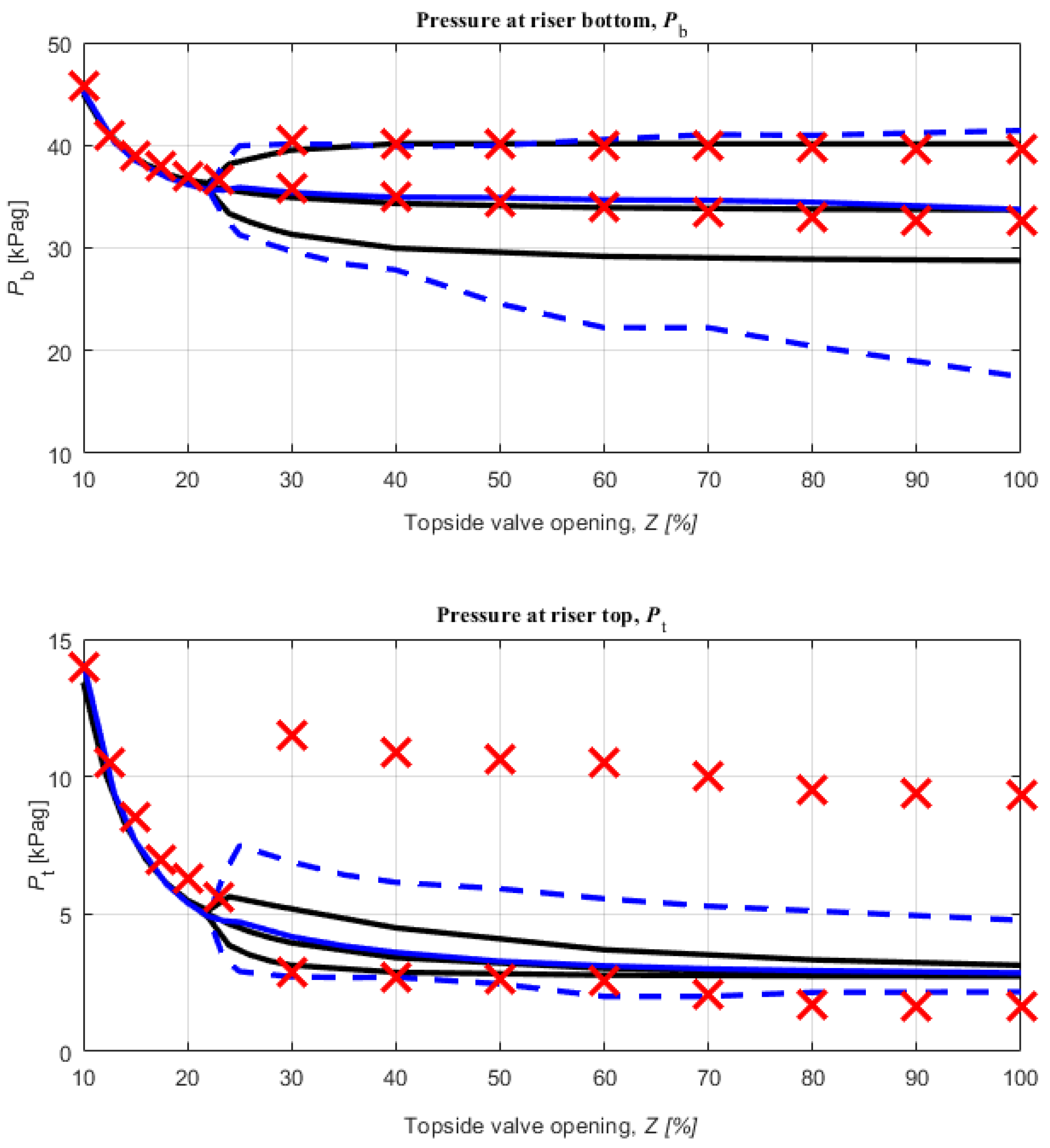
The bifurcation map of the low-dimensional (black) and OLGA model (blue) are compared with the measured pressure data (red) in
Figure 3. The bifurcation map only plots the steady-state results, however it can be a useful tool to compare and validate models’ steady-state performance. It is observed that the open-loop measured bifurcation point (
) fits both models reasonably well, however, the pressures in both models vary from the measured data. At the
-plot the OLGA model seems to have a decreasing minimum peak, however this was due to high-frequency numerical peaks in the OLGA simulations and the average minimum peak was nearly constant at 28
for
. For
is was hard to make the low-dimensional model fit the slug region with large amplitudes observed from the lab measurements. Thus it is clear that even though
is located very close to reality for both models, the models do not fit the measurement well in the slugging region. However the fit of the bifurcation point was weighted over the amplitude peaks in the slug region for the tuning of the models, see
Table 2. The control-oriented model will be used for the controller designs and the OLGA model will be used as a reference model for the controller implementation in
Section 5.


