1. Introduction
The evaluation of wind potential in a region requires systematic data collection and analysis on wind speed and regime. Generally, a rigorous assessment requires specific surveys of the region where the wind farm will be placed [
1,
2,
3]. There are three major markets for the field of global wind power generation: Europe, USA and China [
4]. Wind energy penetration levels continue to rise, led by Denmark with a 40% use of this energy, followed by Uruguay, Portugal and Ireland with over 20%; Spain and Cyprus with about 20%; Germany with 16%; and the major markets of China, the US and Canada with 4%, 5.5% and 6% wind energy, respectively. The forecast of five years ahead is almost 60 GW of new wind power installations in 2017, rising to an annual market of 75 GW by 2021, and an accumulated installed capacity of more than 800 GW by the end of 2021 [
5]. Wind energy is a clean and renewable alternative for the production of electric energy, presenting great social acceptance [
6]. In the social feature, wind power plants do not cause major environmental impacts such as in hydroelectric plants and allow the compatibility between the production of electricity from the wind and the use of land for livestock and agriculture.
Wind generation occurs through the contact of the wind with the blades of the wind device. When rotating, these blades convert wind speed into mechanical energy that drives the rotor of the wind generator, which produces electricity. According to [
7], tropical regions receive solar rays almost perpendicularly and are therefore warmer than the polar regions. Consequently, the warm air that is found in the low altitudes of the tropical regions tends to rise, being replaced by a mass of cooler air that comes from the Polar Regions.
Wind is the result of the displacement of air masses, caused by the effects of atmospheric pressure differences between two distinct regions and influenced by natural effects such as continentally, sea level, latitude, altitude, and soil roughness, among others [
8]. According to [
9], wind power temporal series always have non-linear and non-stationary characteristics and therefore it is very difficult to accurately forecast the power generated. In [
10], it is established that accurate wind forecasting is decisive to have a reliable power system. However, the intermittent and unstable nature of the wind speed makes it very difficult to predict accurately. The objective of this paper is to develop a hybrid system composed by ARIMA model and two Neural Networks to forecast wind power. The proposed model was applied to a case study in Brazil, and results are according to reality.
3. Materials and Methods
3.1. Database
The historical series of the meteorological variables used was obtained from national organization system of environmental data (SONDA) of the National Institute of Space Research (INPE). The series begins on 1 January 2004 and ends on 31 May 2017, this database displays the data per minute of the following variables: Air temperature, Air humidity, Atmospheric pressure, Average wind speed, Wind direction. The database provided by SONDA, can be accessed in the URL
http://sonda.ccst.inpe.br/basedados/.
The complementary data were made available directly with station technicians, since the update up to the date studied is not available online. The site decision was made based on the Brazilian wind atlas [
53], and by the analysis of the average speeds presented in the database.
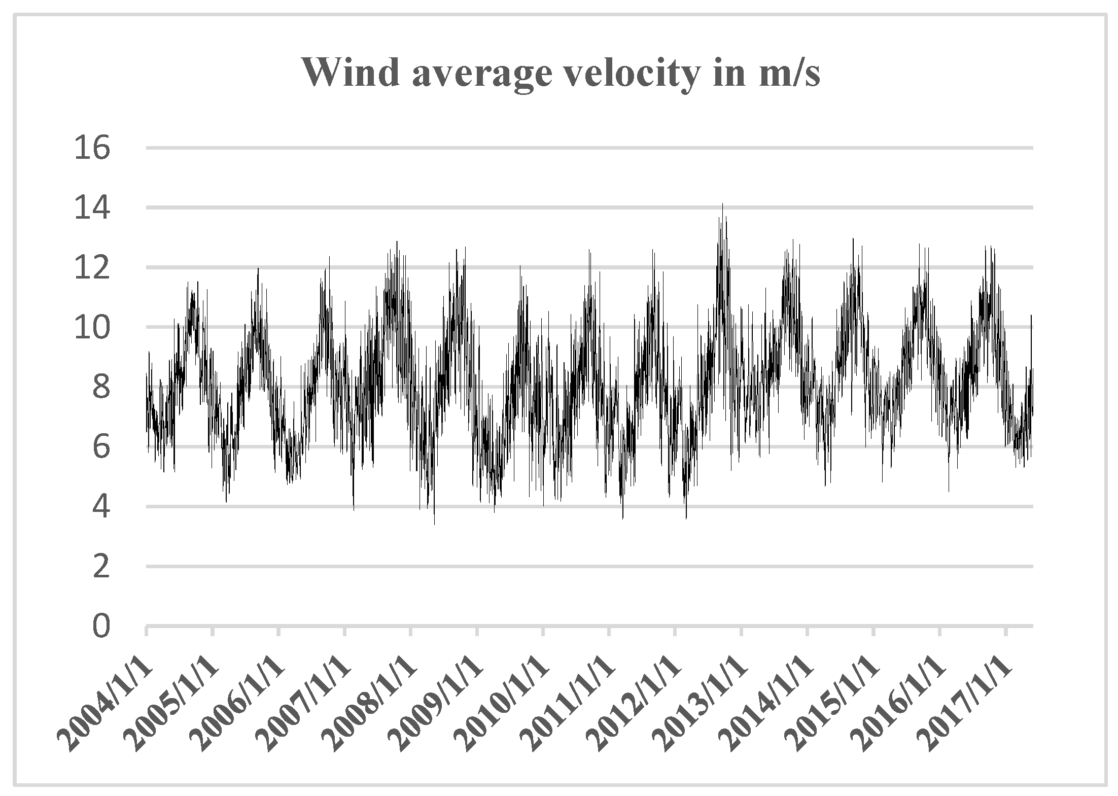
Figure 2 gives an example of the behavior of the time series wind speed of the database.
In this paper, the results obtained for wind speed prediction will be presented using five models: ARIMA, ARIMA + WAVELET, ARIMA + NEURAL NETWORKS 1, ARIMA + NEURAL NETWORKS 1 + NEURAL NETWORKS 2 and NEURAL NETWORKS.
To allow the comparison of the different forecasting horizons, the application of the models follow an equal configuration for all horizons, so it is possible to verify which horizon has the best answer for the proposed model. The configurations will only be applied in the first step of the Model ARIMA. The applications of the neural networks in both the Hybrid model and in the comparative using only Neural Networks will follow standardization as demonstrated after the ARIMA model. The forecasts follow the pattern of
Table 1.
3.2. ARIMA Model
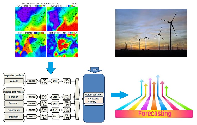
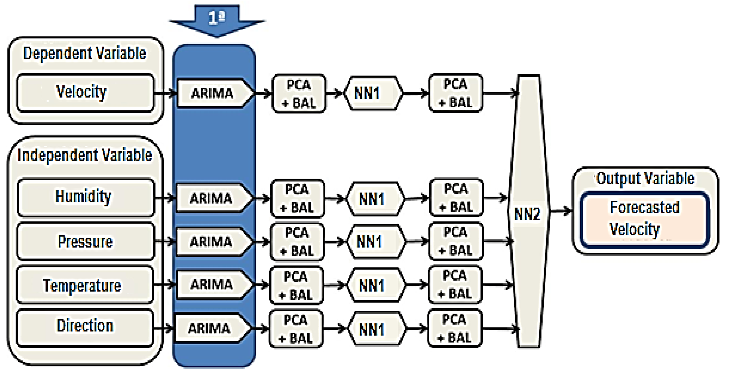
The first step of the proposed algorithm illustrated in
Figure 3 is the ARIMA model (Auto Integrated Regressive of Moving Average), which results from the combination of three filters: the AR component, the Integration filter (I), and the MA component. The representation of this model is done through ARIMA notation of order (p, d, q). An ARIMA (1, 2, 0) representation indicates an order 1 for the AR (Self-Regressive) component, order 2 for component I (Integration or differentiation) and the last 0 for the MA, where: p is the number of seasonal auto-regressive terms; d is the number of seasonal differences; and q is the number of seasonal media moving.
Speed is classified as a dependent variable because its predicted value in ARIMA + NN1 + NN2 depends on the values of the variables humidity, pressure, temperature and direction.
ARIMA models (p, d, q) obtained for each of the time series are presented, respectively, in each application step according to
Table 2.
In this step, the speed dependent variable and the independent variables described above, which are the Humidity, Pressure, Temperature and Direction, generate independent results one of each other. Independence is processed through the program input filter, the time interval of every database used was from 1 January 2004 to 31 May 2017; the estimation is based on the beginning of the data; and the forecast follows the multi pass proposal. First, the response analysis of the models for Step 1 (Minutes, Hours, Days, Weeks, Months, and Years) of each variable was performed. The reliability used was 95% and the delay numbers were 180 for minutes, 72 for hours, 21 for days, 12 for weeks, 38 months and 38 for years. Through extrapolation in the data, these delays represent three cycles of each representation, in order to test the result and then compare it with the variations of the different steps. The initial values found with the ARIMA model represented are the Minimum Error, Maximum Error, Mean Error, Standard Deviation and Linear Correlation. The mean speed of the wind (VMED), mean absolute error (MAE), root mean square error (RMSE), and mean absolute percent error (MAPE) were used to evaluate the prediction accuracy of the variable speed. In [
54], these items are detailed. VMED is the calculation of the average wind speed:
where
N is the number of samples, and
is the actual value of the Speed.
MAE expresses accuracy in the same data units, which helps to conceptualize the magnitude of the error. The equation is:
where,
N is the number of samples,
is the actual value of Speed and
is the speed predicted.
RMSE is a commonly used measurement of accuracy of time series values.
MAPE expresses accuracy as a percentage of the error. Because this number is a percentage, it may be easier to understand than other statistics. For example, if the MAPE is 7, on average, the forecast is incorrect at 7%. The equation is:
Values by themselves cannot demonstrate positive or negative results these values are basis for model comparisons.
3.3. ARIMA + NN1 Model
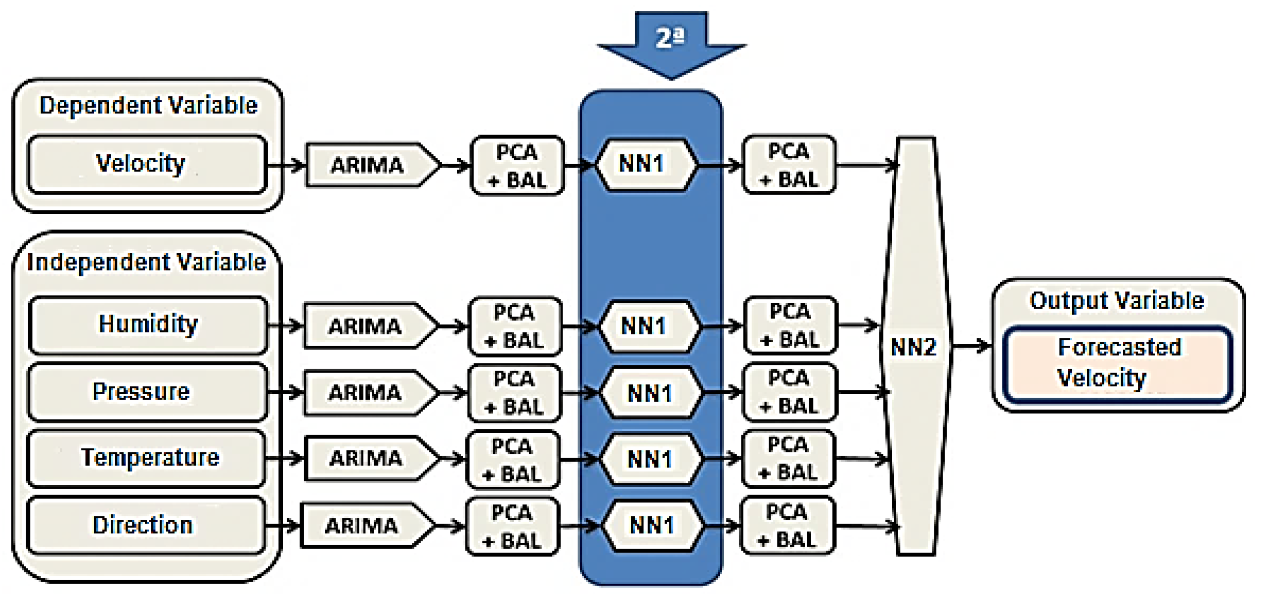
The second step of the model illustrated with the block diagram in
Figure 4 is performed in the first Neural Network—NN1. This step is done to predict explanatory variables and it uses ARIMA results as input variables, which are reduced through the principal component analysis (PCA), which finds linear combinations of the input fields reducing the components for using the main variables.
The NN1 presents eight neurons in the input layers, two neurons in the hidden layer and one neuron in the output layer, configuration used for all variables. The back propagation error training algorithm was used, which adjusts the network weights in order to minimize the error between the actual values and the predicted outputs.
Data partitioning was 80% for training and 20% for testing. The stopping criterion used is the maximum training time per model. The network was trained with sigmoidal tangent activation function for all neurons.
The network follows a standardized programming with multilayer perceptron (MLP) with the topology 8-2-1, logistic activation function and back propagation algorithm. The network uses the data for each respective horizon, i.e., 180 for minutes, 72 for hours, 21 for days, 12 for weeks, 38 months, and 38 for years by applying the extrapolation in the data. These delays signify three cycles of each representation, and project one step forward, the recursive network re-inserts each projection at the input of the MLP and does that repetition automatically 20 times. In this step, the ARIMA + NN1 speed prediction is made and all values are analyzed based on errors, standard deviation and linear correlation.
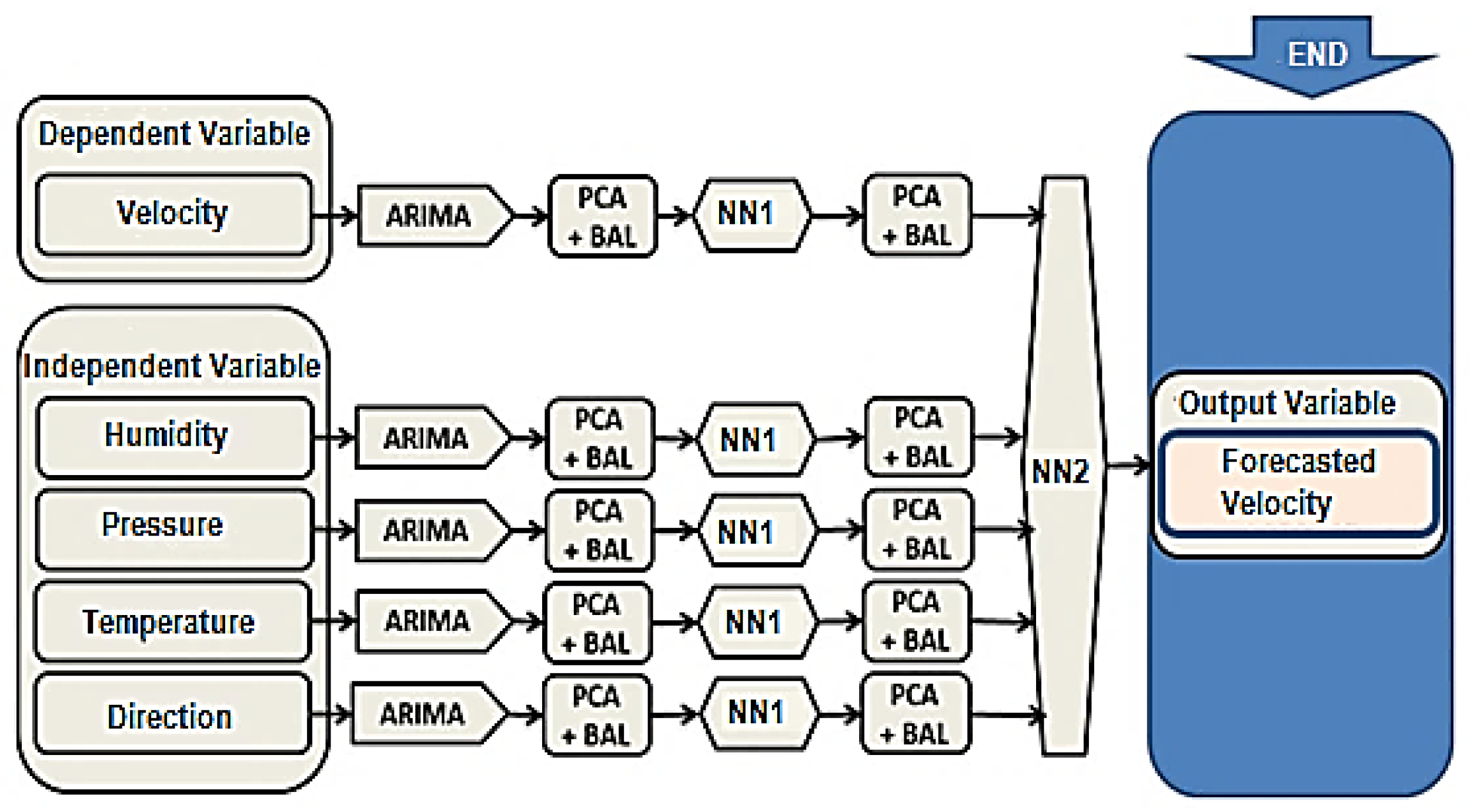
3.4. ARIMA + NN1 + NN2 Model
The final step of the algorithm is represented by the block diagram in
Figure 5. In this step, the final speed prediction is made.
The NN2 uses the outputs of the ARIMA + NN1 model as input to optimize the results, which adjusts the weights of the neural network in for minimizing the error between the actual values and the predicted outputs. Data partitioning was 80% for training and 20% for testing.
The network follows a standardized programming with MLP with the topology of 11 neurons in the input layer, eight neurons in the hidden layer and one neuron in the output layer, logistic activation function and back propagation algorithm. It uses values for each respective horizon; that is, 180 for minutes, 72 for hours, 21 for days, 12 for weeks, 38 months, and 38 for years by applying extrapolation to the data. These delays signify three cycles of each representation. They project one-step forward; the recursive network re-inserts each projection at the input of the MLP and do this repetition automatically 20 times.
The stopping criterion is the maximum training time per model. The network was trained with sigmoidal tangent activation function for all neurons.
3.5. Neural Networks Model
The model of neural networks was used to compare the results obtained by the proposed hybrid model; the configuration of the model has as input the environmental data of real values described as input variables.
The network follows a standardized programming with MLP with the topology formed with nine neurons in the input layer, seven neurons in the hidden layer and one neuron in the output layer, logistic activation function and backpropagation algorithm. It uses values for each respective horizon, that is, 180 for minutes, 72 for hours, 21 for days, 12 for weeks, 38 months, and 38 for years by applying extrapolation to the data. These delays represent three cycles of each representation, and project one step forward, the recursive network re-inserts each projection at the input of the MLP and does this repetition automatically 20 times.
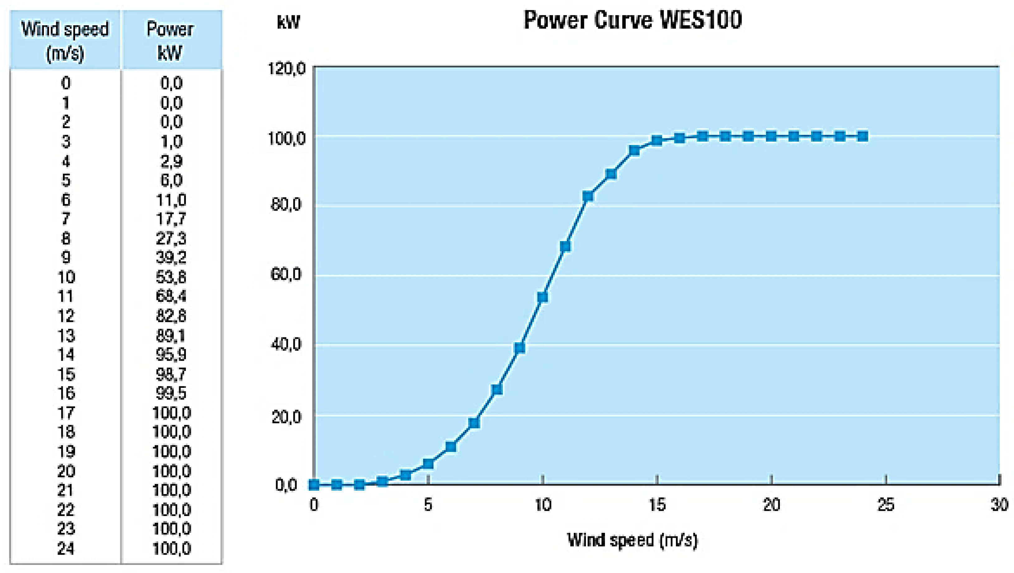
3.6. Forecast of Wind Speed and Generated Power
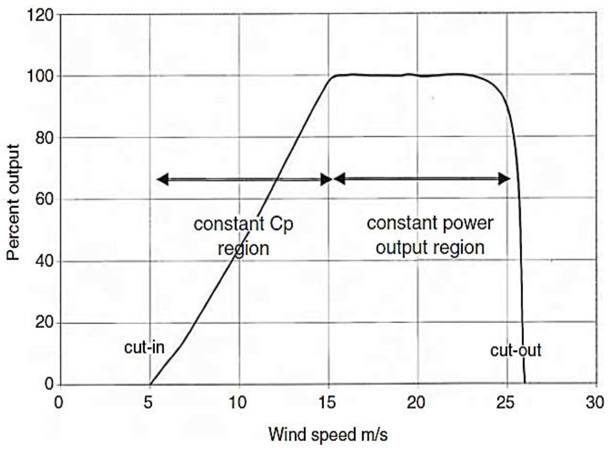
The final objective of this work is to forecast the wind speed to predict the generated power. For a given wind speed, the power generated depends on the type of generator to use. The wind turbine chosen for the study was the WES100 model with 100 kW of power, capable of generating 100 kW at an average wind speed of (17 m/s),
Figure 6 shows the power curve of the wind turbine.
To obtain the generator power curve equation, curve expert software was used from the Power and Speed data. The equation that represents the generation curve is given by:
where
P = Generated Power;
x = Wind Speed;
a = 1.515151515153736 × 10
−2;
b = −6.414141414141929 × 10
−2;
c = −9.734848484848370 × 10
−2;
d = 8.005050505050480 × 10
−2; and
e = −1.893939393939385 × 10
−3.
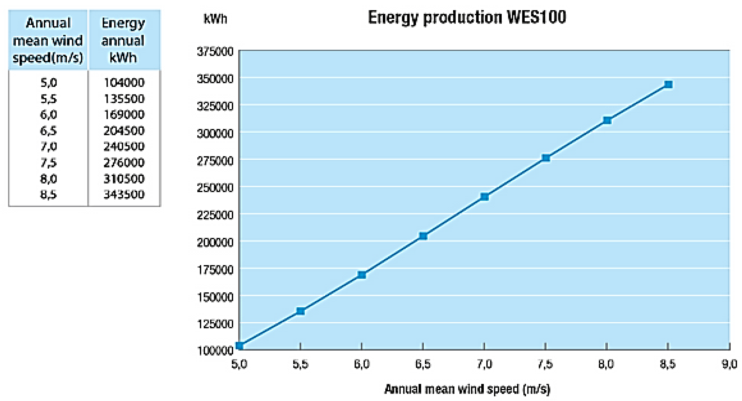
Figure 7 shows the graph of annual generation of wind turbine generator wind energy solutions (WES) 100 in kWh.
To obtain the energy curve equation provided by the generator, curve expert software was used from the Energy and Speed data. The annual energy equation generated according to the wind speed for this turbine is:
where
E = Generated Energy;
v = wind speed;
a = 5.738920454544906 × 10
5;
b = −3.862506313128678 × 10
5;
c = 9.348295454540566 × 10
4;
d = −8.406565656562561 × 10
3; and
e = 2.803030303030391 × 10
2.
4. Result Analysis
The results obtained will be shown for each forecast universe as described above. In the case of wind speed, there were used symmetric daubechies wavelets combined with ARIMA model for the forecast.
4.1. Ultra Short Term Forecast—CPU (Minutes)
The data used have a base containing 7200 rows, and a total of 36,000 data; such amount is equivalent to a universe of five days.
The multi-step ahead results show that some of the used models have a significant loss of precision, the higher the prediction step, the lower the precision. The ARIMA model already starts with very large errors, the absolute mean error for example in 5-min steps is 0.795 and the MAE percentage is 15.024%. For 20-min steps, the absolute mean error becomes 1.182, and the mean absolute percentage error reaches 20.591%. However, because the ARIMA model returns the prediction values with one-step delay, it will always be worse than the model with neural networks. The ARIMA + NN1 + NN2 model in the step forecast or 5 min, obtained an absolute mean error response of 0.199 and an absolute mean error response of 3.620%. For prediction of 20 min steps, the absolute mean error goes to 0.308 and the mean absolute percentage error goes to 5.305% (see
Table 3); this result is superior to the other models, confirming its performance (see
Table 3).
The values presented in the table above show the results for each model. The results of ARIMA tend to predicted average based on the delay and the values with intervention of the model of neural networks are based on non-linear characteristics. The actual values were obtained until 31 May 2017, the forecast was made from the Minute 00 of 1 June 2017 extending to the 20th min of the same date; that is, a forecast of 20 step (minutes) forward.
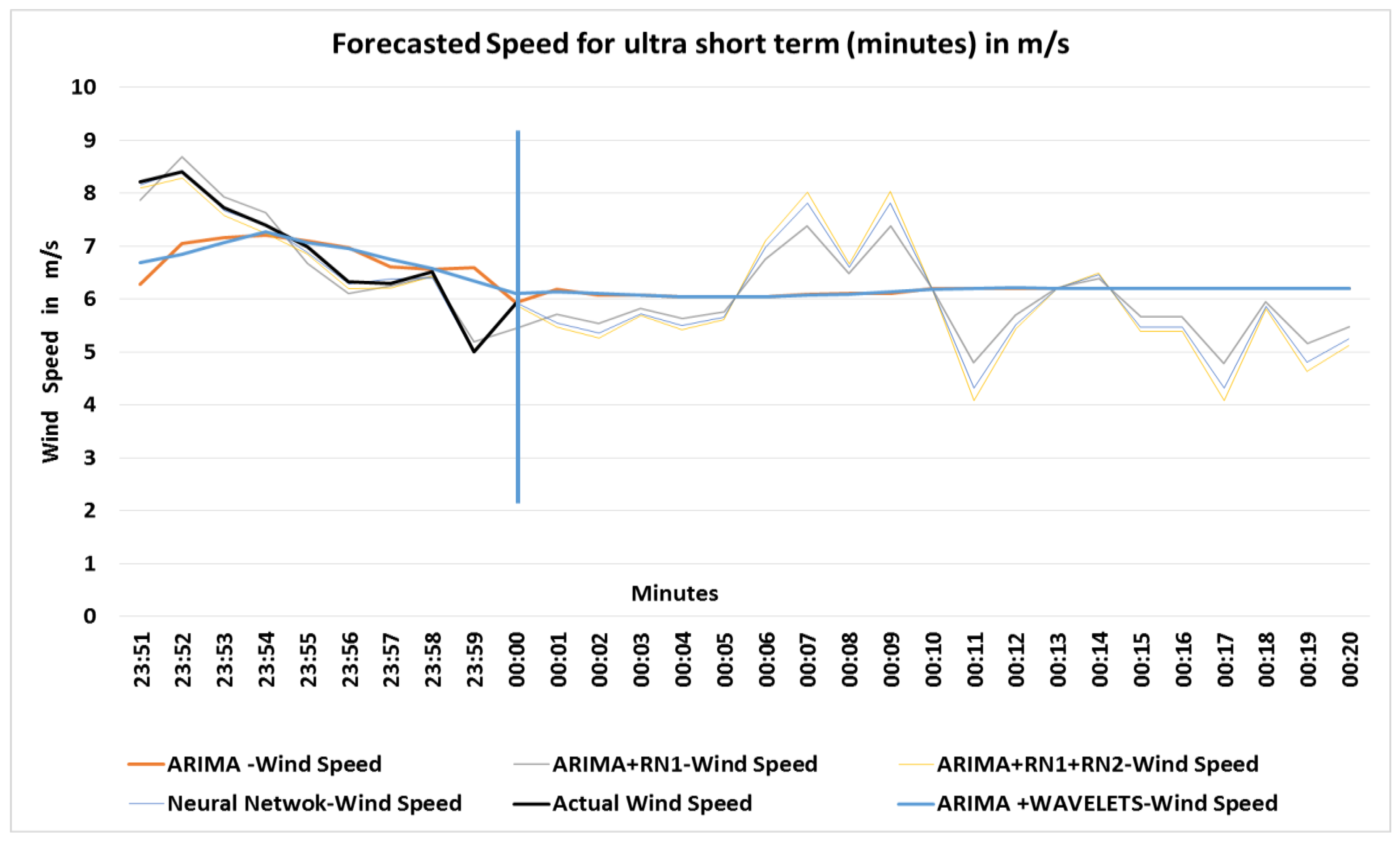
4.2. Forecasted Speed at Ultra-Short Term (Minutes)
Figure 8 shows the results of the speed values in m/s predicted for ultra-short term in minutes.
In
Figure 8 it can be appreciated that there is no great difference between ARIMA model and ARIMA + WAVELETS model, and the latter one will not be included in power and energy forecasting.
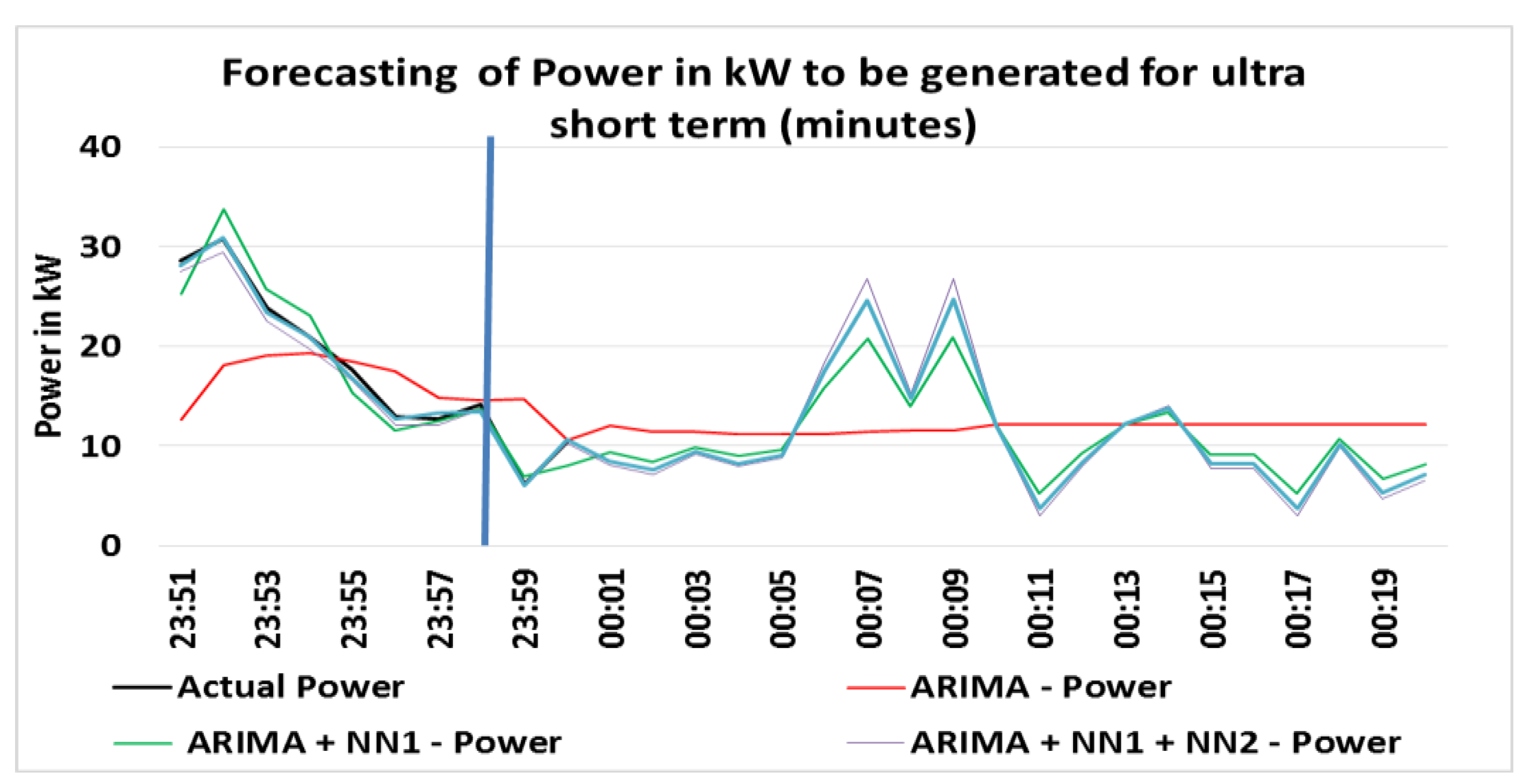
4.3. Estimated Power at Ultra-Short-Term (Minutes)
Figure 9 shows the generated power predicted for ultra-short-term (minutes); the results data are in KW.
The forecast for this horizon takes into account an ultra-short time interval, which produces some abrupt changes in the speed variation. From the interval of 5 min to 7 min, there was an increase of approximately 15 kW according to the forecast ARIMA + NN1 + NN2, and a drop of approximately 20 kW from the range of 9 min to 11 min. After these peaks, forecasting tended to an average of approximately 10 kW and the ARIMA model tended to 12 kW. There were peaks in the prediction of up to 26 kW. The forecast of power generation for this horizon is important for electricity market compensation, real-time network operations and regulatory actions.
4.4. Short Term Forecast—(Hours)
It was also performed the short term forecast that covers the magnitude of time in hours. The data used for this horizon have a base containing 8760 lines, and a total of 43,800 data, these data are equivalent to a universe of 1 year.
Table 4 shows the errors in the values of predicted speed for short term forecast.
The short-term results show outcomes proportional to the ultra-short term results where the ARIMA model obtained a good result, and the neural network model was superior. The second stage of the ARIMA + NN1 model had a subtle improvement, and the Proposed Hybrid Model ARIMA + NN1 + NN2 is superior to the other models with results. Although the correlation in the Neural Networks model was subtly superior to the proposed Hybrid model, the result of the mean absolute error (MAE) has greater weight in the consideration of the best model. Nevertheless, the RMSE is also important because it shows the average magnitude of the estimated errors, has always positive value and the closer to zero, the higher the quality of the measured or estimated values. The smaller the discrepancy of the data, the better is the result. The ARIMA + NN1 + NN2 model returns a higher accuracy than other ones.
In
Table 4, the results of errors in speed prediction for ultra-short term for 5 h, 10 h and 20 h for ARIMA, ARIMA + NN1, ARIMA + NN1 + NN2 and Neural Networks models are presented.
The average speed (VMED) results for the various prediction steps are very close due to the wind behavior which although varying throughout the day, the average takes into account all previous values. For example, the speed for five steps or 5 min in the ARIMA model is 7.562 m/s; this average is the sum of the values divided by the number of samples, in the 20-step or minute forecast the average speed is 7.306.
Although the speed is very close, the ARIMA model has a characteristic that tends to mean moving average of the data, even with this characteristic of the behavior of the average speed and the characteristic of the model, the average percentage error (MAPE) returns a very high value of forecast. In this forecast horizon for short-term (hours) multi-steps ahead, the ARIMA + NN1 + NN2 model in both the absolute mean error, the mean square error, and the mean error, obtained a better result than the other models.
4.5. Wind Speed Short Term Forecasting (Hours)
Figure 10 shows the results of the speed values in m/s predicted for short term forecasting in hours.
In
Figure 10, it can be appreciated again that there is not a great difference between ARIMA model and ARIMA + WAVELETS model.
The actual values are until 31 May 2017, the forecast was made from Hour 01 of 1 June 2017 extending up to 20 h at the same date; that is, a forecast of 20 step (hours) forward.
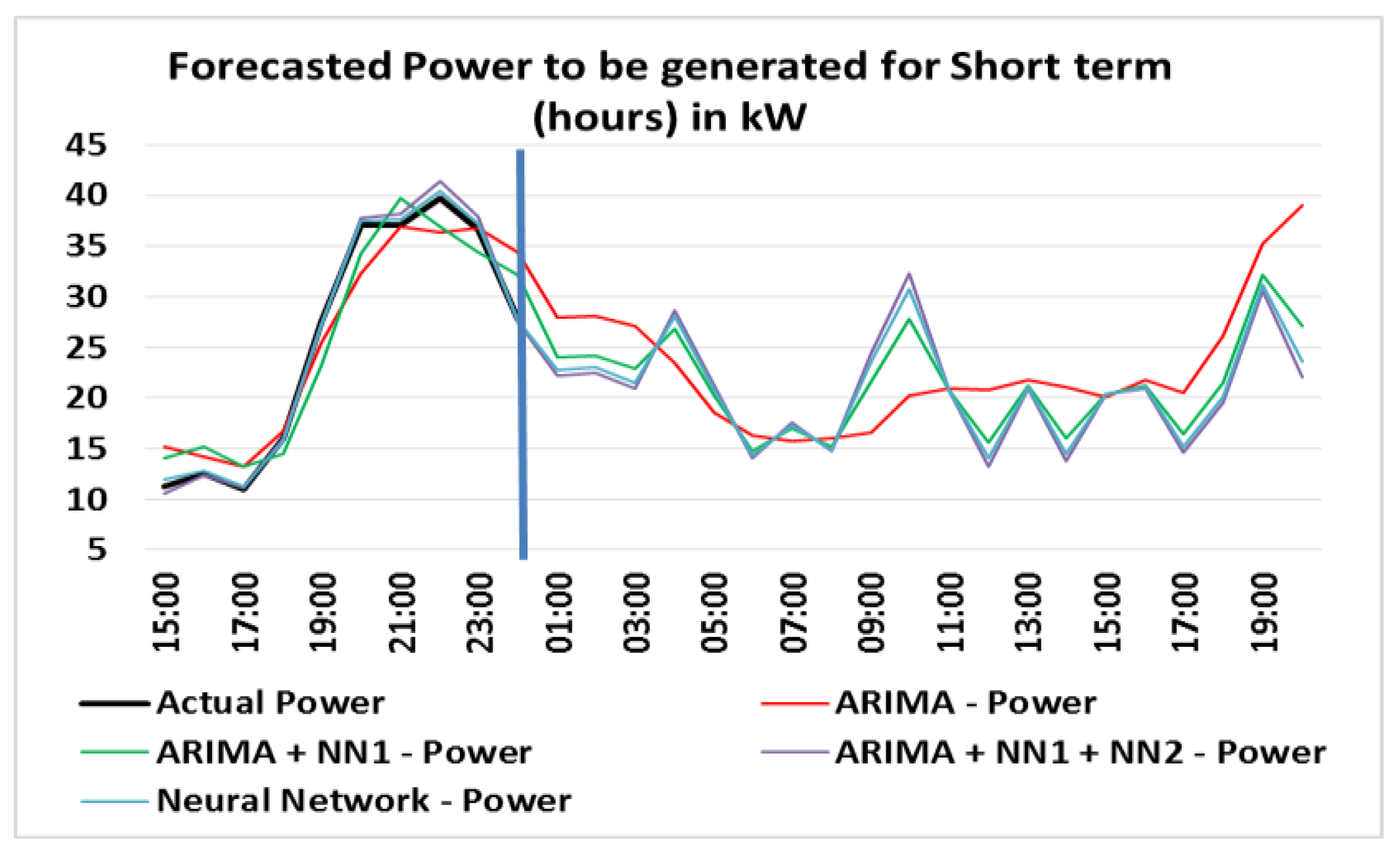
4.6. Short Term (Hours) Forecasted Power in kW
Figure 11 shows the expected generated power for short term (hours); the results are given in kW.
The generated power varies according to the expected wind speed, for the selected generator. For this generator can be generated a power of up to 40 kW. This power can be increased taking into account the speed and also adopting a wind generator of more capacity. The variation in the power generation prediction behavior was smoother than the ultra-short prediction, but there was still a variation of approximately 15 kW from the range of 8–10 h and a decrease in the same proportion in the 10 h for 12 h interval
This forecast horizon is important for planning the economic load dispatch, reasonable load decisions and operational safety in the electricity market.
4.7. Medium Term Forecast (Days)
The data used for this horizon, have a base containing 8736 lines, and a total of 43,680 data. These data are equivalent to a universe of 13 years.
All values of errors are considered important in the result analysis. For the medium term, the proposed Hybrid model ARIMA + NN1 + NN2 has a better result than other models. In
Table 5, the results of the errors for Medium Term for 5 days, 10 days and 20 days are presented for ARIMA, ARIMA + NN1, ARIMA + NN1 + NN2 and Neural Networks models related to the speed predicted.
Results show that even the highest 20 h forecast for the ARIMA + NN1 + NN2 model is superior to the lower ARIMA and ARIMA + NN1 prediction, showing the efficiency of the proposed model.
4.8. Medium Term Forecasted Speed (Days)
Figure 12 shows the results of the speed values in m/s predicted for medium term in days.
The actual values are until 31 May 2017, and the forecast was made from 1 June 2017 extending through 20 June 2017 with 20 steps (Days) forward.
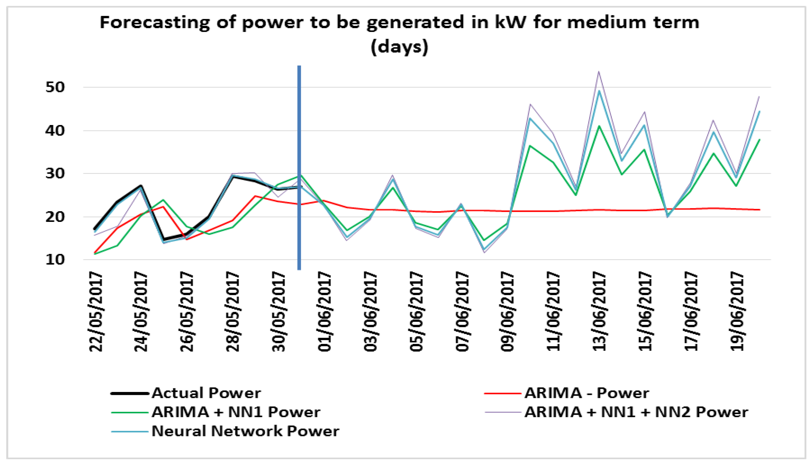
4.9. Estimated Power for Medium Term (Days)
Figure 13 shows the expected power generated for the medium term. The results are given in KW.
The calculated actual values are until 31 May 2017, and the forecast was made from 1 June 2017 and extended until 20 June 2017 with 20 steps (days) forward. The variation of the generation capacity of the horizon days is greater in relation to the hour horizon. This is due to the behavior of the winds, which although not being part of the analysis of this paper, deserves an observation since the wind repeats its behavior during the cycle of one day, one month and one year, on proportional scales. It is possible to realize that there were generation peaks of more than 50 kW, close to 60% of the maximum capacity of the wind turbine. This generation value could increase if another wind generator of greater capacity would be used. The medium-term forecast horizon is important for unit commitment decisions, reserve commitment decisions and generator online/offline decisions.
4.10. Medium Term Forecast (Weeks)
The fourth forecast horizon was performed over the medium term, which covers the time quantity in weeks. The data used have a base containing 1248 rows, and a total of 6240 data, and such amount is equivalent to a universe of 13 years.
Results for the medium-term forecast show that the ARIMA + NN1 + NN2 hybrid model is superior both in relation to the compared models and in comparison, to the horizons already shown, the linear correlation keeps the result very strong considering the Pearson coefficient. The MAPE obtained shows a better result for this horizon due to the forecasted speed behavior. The mean absolute percentage error. The results of the errors in predicted speed for the medium term for 5 weeks, 10 weeks and 20 weeks for the ARIMA, ARIMA + NN1, ARIMA + NN1 + NN2 and Neural Networks models are presented in
Table 6.
Although, in the prediction of one step (week), the hybrid model proposed ARIMA + NN1 + NN2 had a loss of precision in relation to the medium term horizon forecast (days), these variations are relative to the statistical behavior of the data.
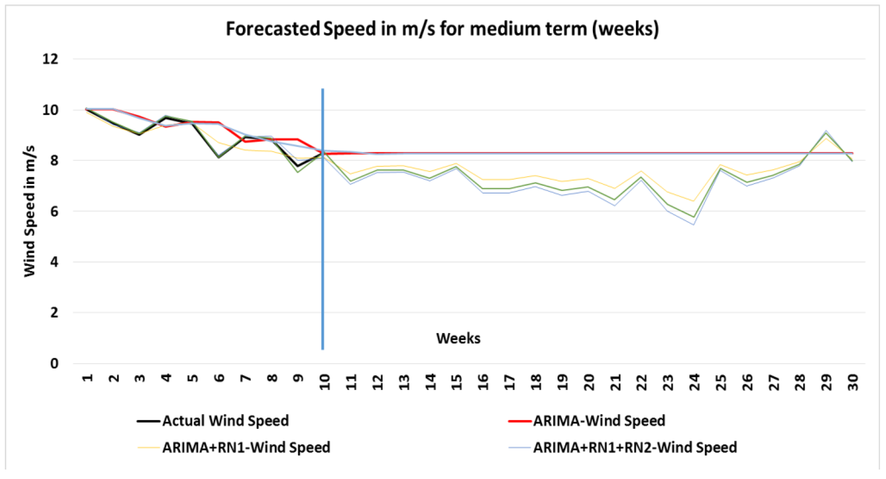
4.11. Predicted Wind Speed in Medium Term (Weeks)
Figure 14 shows the results of the expected speed values in m/s for medium term in weeks.
The actual values are up to 31 May 2017, and the forecast was made from 1 June 2017 extending for 20 weeks, which corresponds to the date of 12 October 2017, with a horizon of 20 step (weeks) forward.
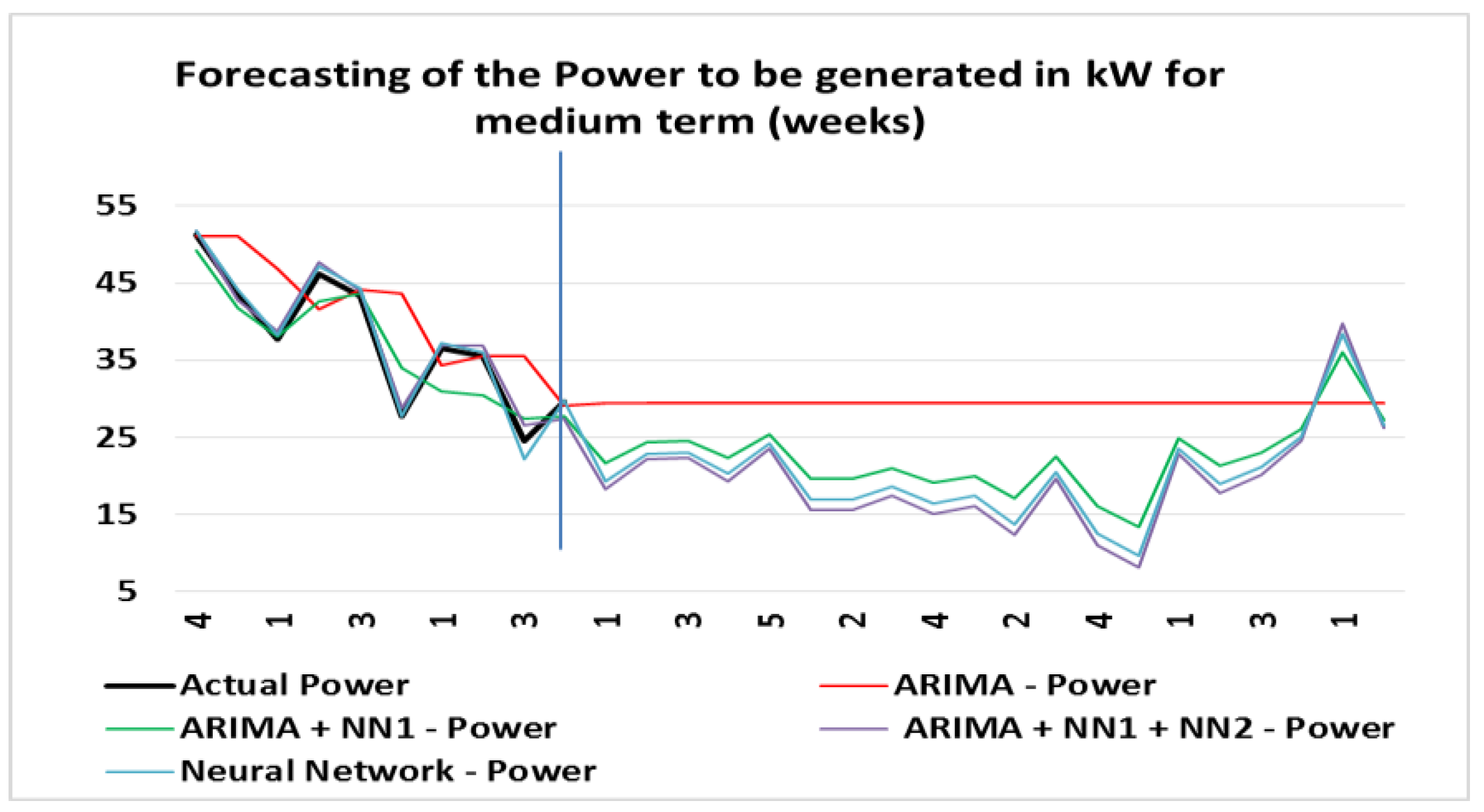
4.12. Estimated Power Medium Term Weeks
Figure 15 shows the expected power generated for medium term (weeks); results are given in KW.
Actual calculated values are until 31 May 2017, and the forecast was made from 1 June 2017, extending it 20 weeks forward. Comparing the generation results with the other horizons, it is possible to notice that the behavior varies according to the winds, even though the variations are below 10 kW, the power generation forecast was maintained at an average near 20 kW and with peaks of 40 kW expected. These values may be higher with wind variation or adopting wind generator with higher generation capacity. The medium-term forecast horizon for weeks is also important for unit commitment decisions, reserve commitment decisions and generator online/offline decisions
4.13. Long-Term Forecast (Months)
The fifth forecast horizon was performed in long term, the time quantity in months was used.
The data used have a base containing 312 rows, and a total of 1560 data, which is equivalent to a universe of 13 Years.
The long-term results show an improvement in the results in the proposed ARIMA + NN1 + NN2 hybrid model, which is superior both in relation to the compared models and in comparison, to the previous horizons, the linear correlation has a result considered perfect according to the Pearson’s coefficient. These values have higher results than the multi-step forecast, since these represent responses to one-step only.
Table 7 presents the results of the long-term errors in predicted speed for 5 months, 10 months and 20 months for the ARIMA, ARIMA + NN1, ARIMA + NN1 + NN2 and Neural Networks models.
The ARIMA + NN1 + NN2 hybrid model maintained the same evolution of the medium term horizon (weeks), which had the best performance in relation to the previous horizons, but had a loss of precision in multi steps.
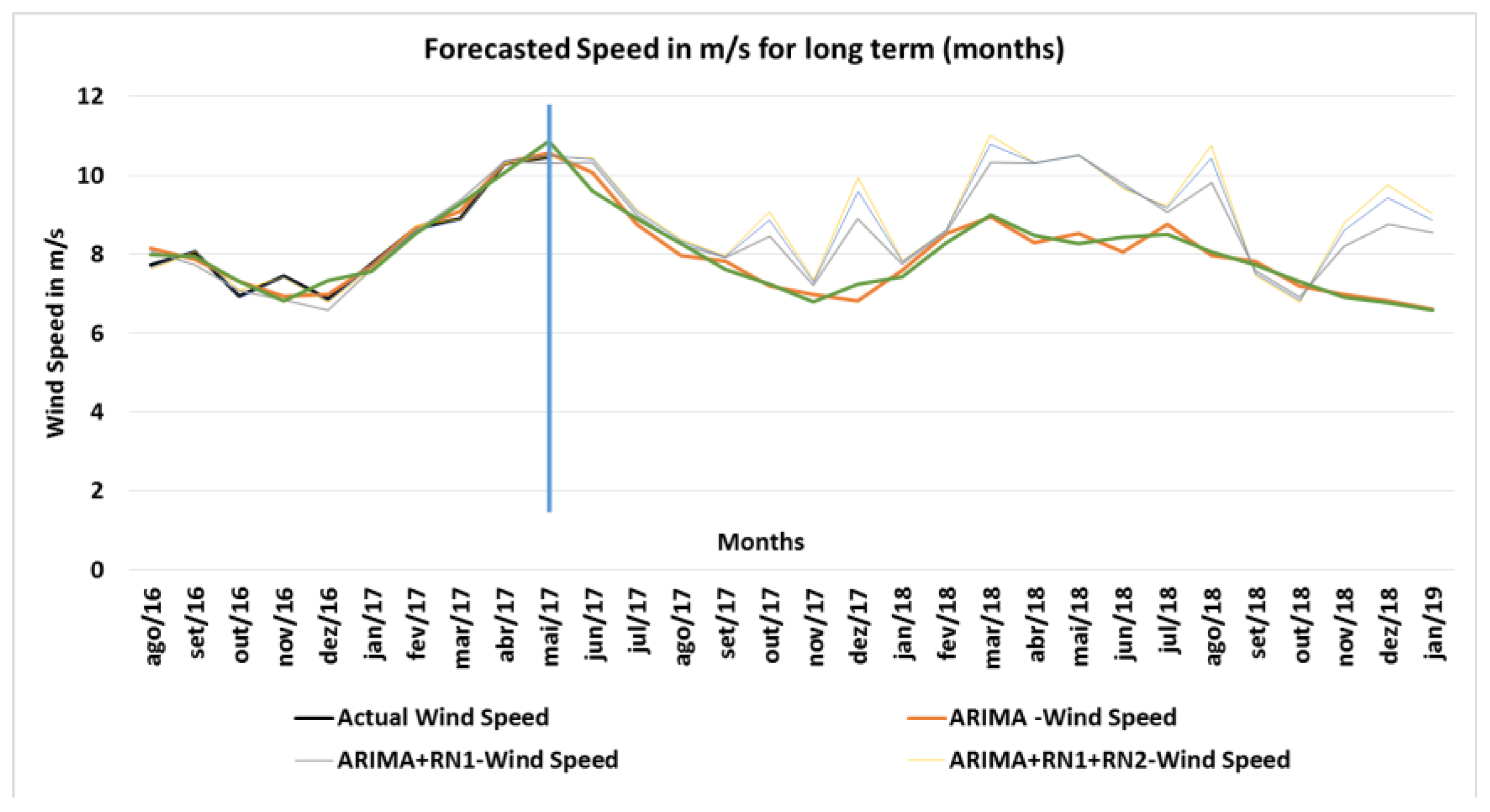
4.14. Long-Term (Months) Forecast Speed
Figure 16 shows the results of the speed values in m/s predicted for long term in months.
The actual amounts are up to 31 May 2017, the forecast was made from 1 June 2017 and it was extended for 20 months, covering until January 2019, a horizon of 20 step (months) forward.
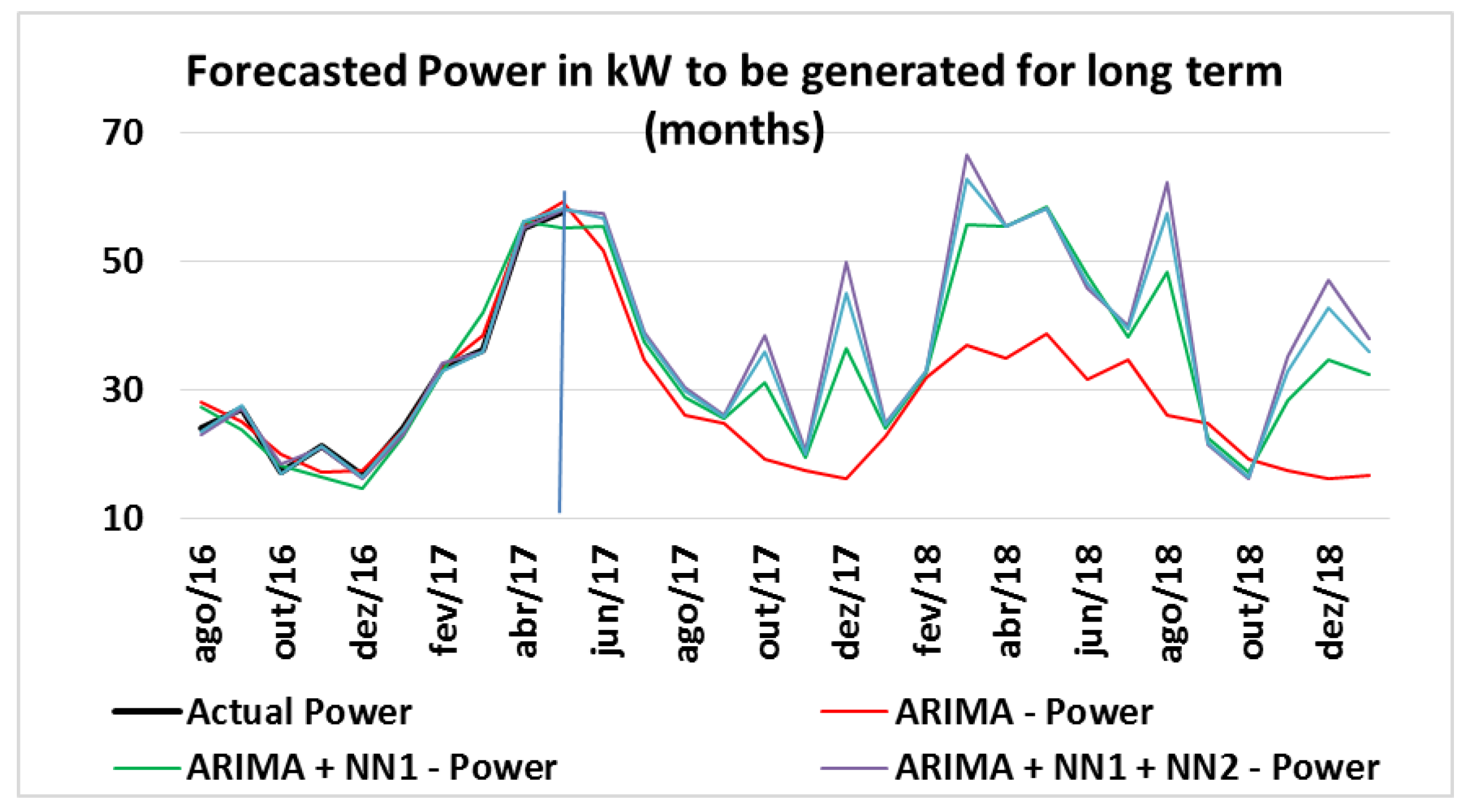
4.15. Long-Term (Months) Forecasted Power
Figure 17 shows the generated power expected for long term (months); the results are given in KW.
Actual calculated values are until 31 May 2017, the forecast was made from 1 June 2017, and it was extended 20 months forward. In this horizon, the forecast amplitude of the generated power is greater, due to the wind behavior, which varies the complete cycle, in April, May and June. There were obtained peaks of more than 60 kW of predicted power, almost 70% of the total capacity of the wind generator. If another higher capacity generator replaces the generator, the power generation will also be higher. The long-term forecast horizon is important for maintenance planning, operation management, optimum operating cost, and feasibility study of wind farm projects.
4.16. Long-Term Forecast (Years)
The sixth forecast horizon was performed in the long term, the time quantity was used in years.
For the long-term horizon of magnitude in years, because the database has only 13 rows, which is considered insufficient to make a forecast with the models and techniques proposed, the base of months was used, which contains 312 rows, with a total of 1560 data. This amount is equal to a universe of 13 years. After the application of the models was done, the interpolation of the data transforming the results from months to years, and for comparison of the results, the extrapolation was also used through the moving average of the data in years to enable the comparative tests to be carried out.
The results for long term in years have similar behavior to the other horizons keeping the proposed Hybrid Model ARIMA + NN1 + NN2 with superior performance compared to the other models analyzed.
Table 8 presents the results of the five-year long-term errors for the ARIMA, ARIMA + NN1, ARIMA + NN1 + NN2 and Neural Networks models. For this horizon, it was only possible to forecast for five-steps (years) due to limited database of 13 years.
The result for the long-term horizon in years had a great performance even having a very small database; the result was possible using statistical and mathematical techniques of extrapolation and interpolation and due to the consistency of the applied models.
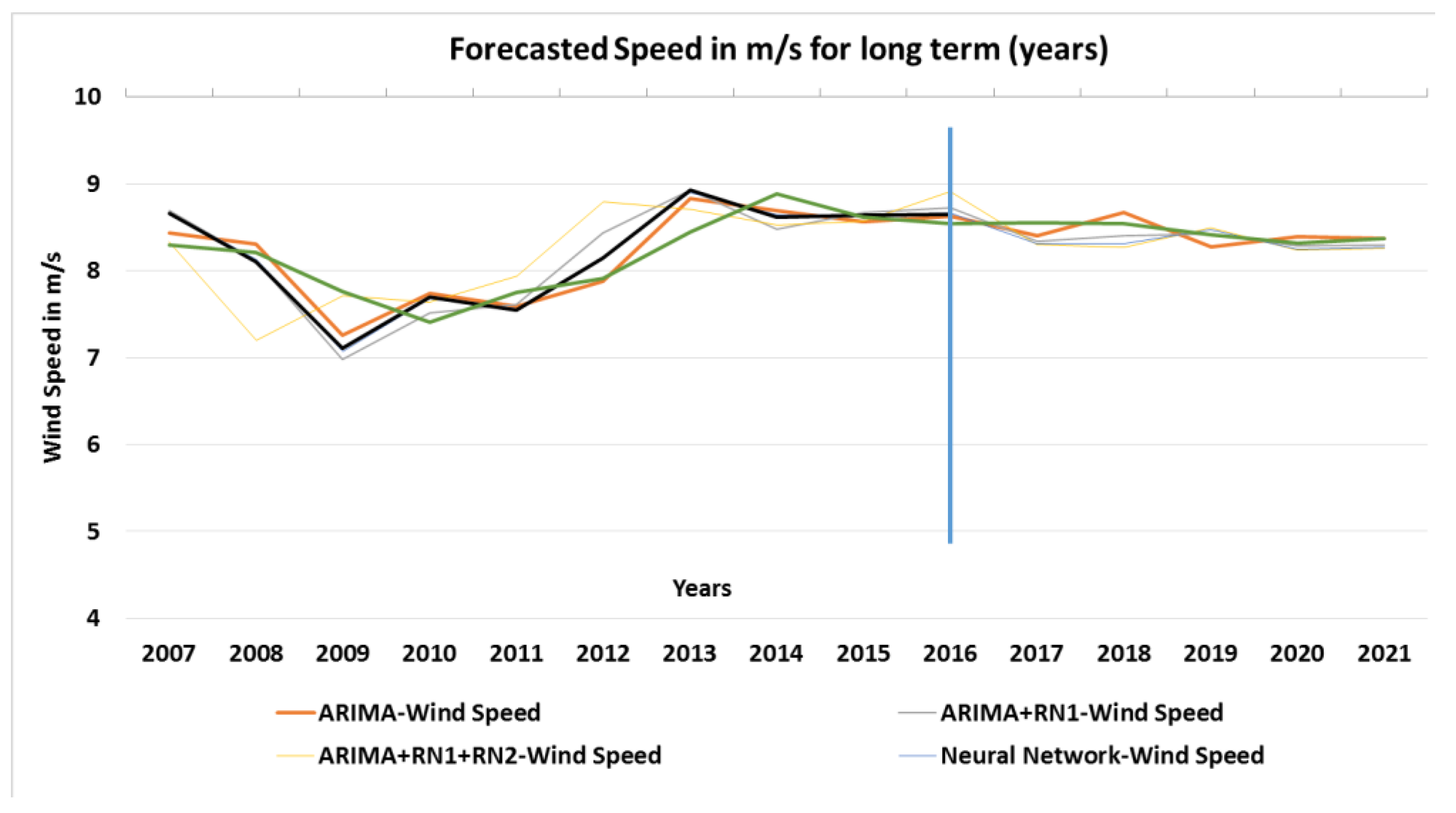
4.17. Long-Term Forecasted Speed
Figure 18 shows the results of the speed values in m/s predicted for Long Term forecast in years.
The actual values are until 31 December 2016, the forecast was made from 1 January 2017, and it was extended for five years, covering until 2021, which is a horizon of 20 steps (years) forward. The annual speed has a smaller variation than the velocities of the other horizons, since the wind has a variation according to the seasons of the year, but this paper does not intend to treat this subject.
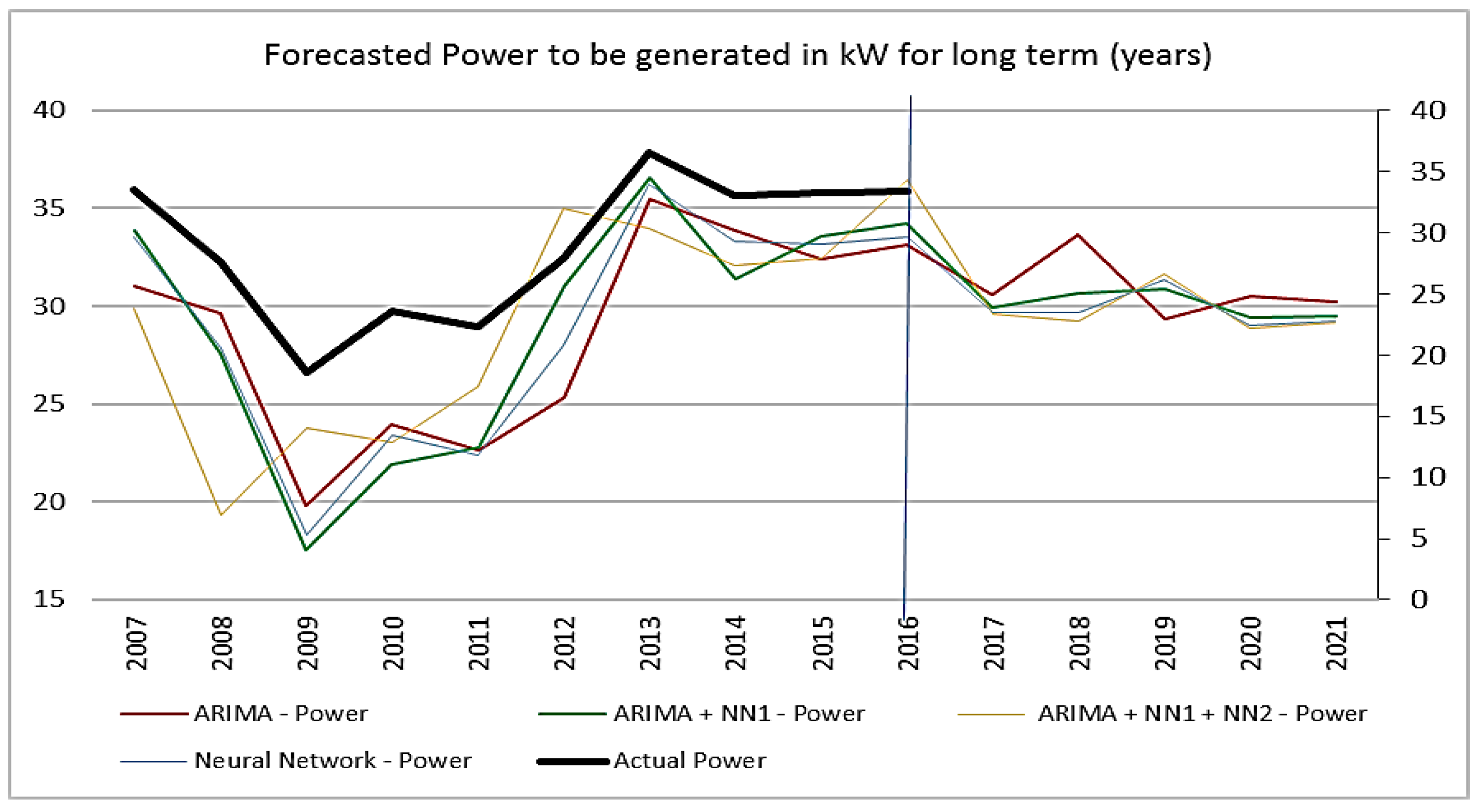
4.18. Long-Term (Years) Power Generation Forecast
Figure 19 shows the power generated predicted for long term (years) forecast; the results are given in kW.
The calculated actual values are until 31 December 2016, the forecast was made from 1 January 2017, and it was extended five years forward. This forecast horizon extends for five steps or five years; it is a lower forecast than the previous horizons due to the amount of historical data. However, it is possible to perceive that the amplitude of forecast of generation is greater, due to the behavior of the wind the in the months of April, May and June, with peaks of more than 60 kW of expected power, almost 70% of the total capacity of the wind generator, if the generator is replaced by a larger one, the power generation will also be bigger. The long-term forecast horizon for steps in years is important for maintenance planning, operation management, optimum operating cost and feasibility study for wind farm projects.
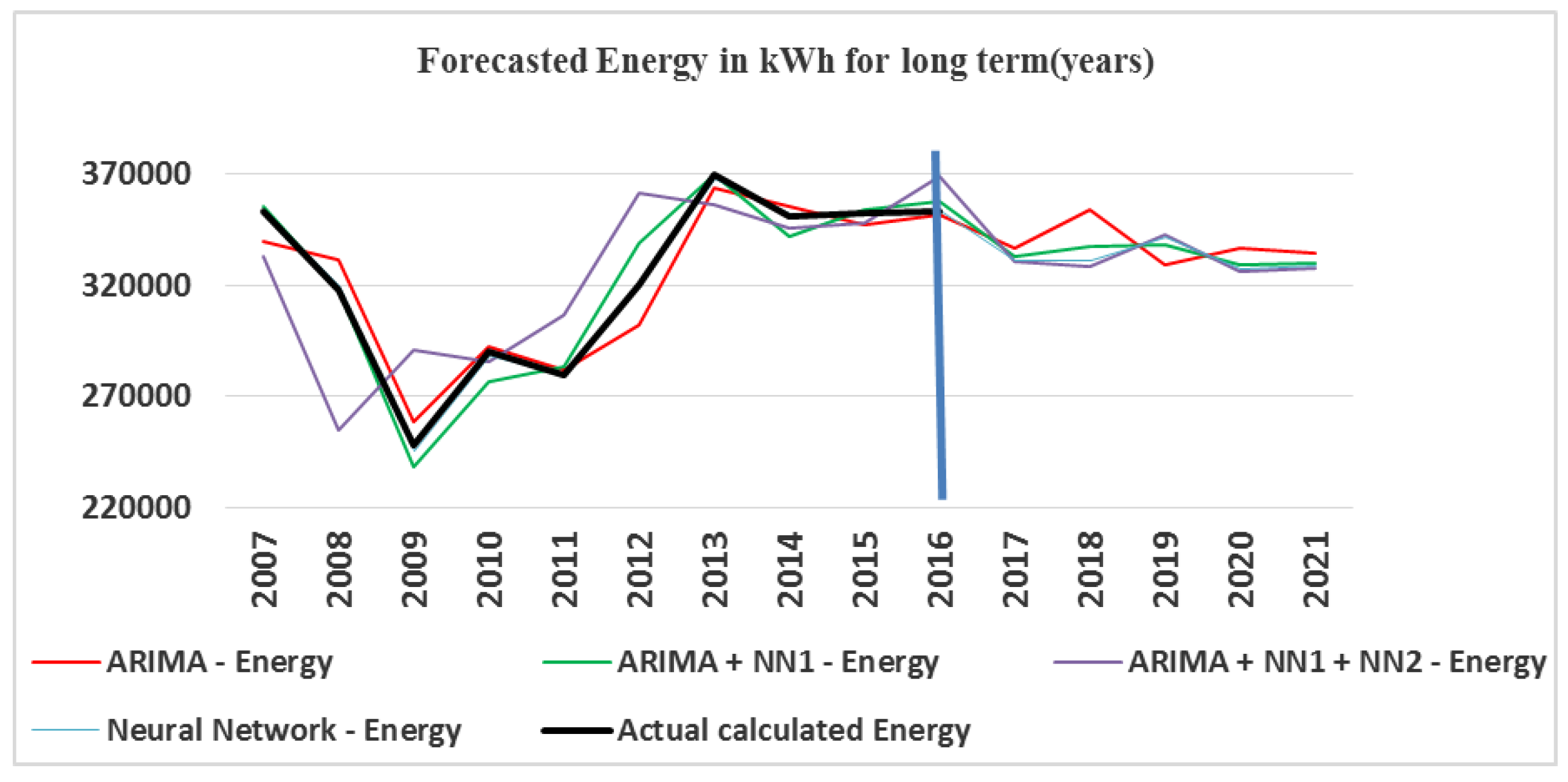
4.19. Average Yearly Energy Predicted for Long-Term Forecast (Years)
Figure 20 shows the predicted average annual energy forecast for long-term horizon (years); the results are given in kWh.
The energy forecast for the horizon shows a peak of approximately 365,000 kWh for the ARIMA model and 362,000 kWh for the ARIMA + NN1 + NN2 model, the amplitude of the forecast is not very large, and does not have very abrupt forecast variations.


 ,
, 


