The Use of an Improved LSSVM and Joint Normalization on Temperature Prediction of Gearbox Output Shaft in DFWT

1
School of Mechanical, Electronic and Control Engineering, Beijing Jiaotong University, Beijing 100044, China
2
Department of Electrical Engineering, North China Electric Power University, Baoding 071003, China
*
Author to whom correspondence should be addressed.
Energies 2017, 10(11), 1877; https://doi.org/10.3390/en10111877
Submission received: 20 September 2017
/
Revised: 4 November 2017
/
Accepted: 5 November 2017
/
Published: 16 November 2017
Abstract
:In the working process of Double-Fed Wind Turbines (DFWT), it is very important to monitor and predict the temperature of the high-speed output shaft of the gearbox timely and effectively. Support vector machine has more advantages in the temperature prediction of wind turbines. Least squares support vector machine is suitable for online prediction due to reducing the computational complexity of support vector machine. In order to solve the sparsity of least squares support vector machine, an improved least squares support vector machine based on pruning algorithm is proposed in this paper to predict the temperature of the high-speed output shaft of gearbox using the practical data of Double-Fed Wind Turbines. At the same time, in order to improve the prediction accuracy and to solve the problem of few links between different feature parameters in common normalization method, the paper uses the method of joint normalization to preprocess the data. The principal component analysis is used to reduce the dimension of the data. Particle swarm optimization algorithm is used to optimize the parameters of the pruning least squares support vector machine. The proposed model that is established in this paper is a new model to forecast the temperature of the high-speed output shaft. The results show that its prediction accuracy is higher than that of other algorithms.
1. Introduction
Wind energy is a kind of clean and renewable energy. Wind energy generation has a positive significance to improving the diversity of energy supply and reducing environmental pollution [1]. At present, the large capacity variable speed constant frequency Double-Fed Wind Turbines (DFWT) are mainly used in the wind farm [2]. The gearbox is one of the most important components of DFWT. It is shown that the maintenance cost for the gearbox is very high when compared with the other higher failure rate components, such as electric system and hydraulic system [3]. So, the timely monitoring of the working state of the gearbox is very necessary. Now, using the temperature information to monitor the abnormal operation of the gearbox is an effective method [4]. High-speed output shaft is the core of DFWT gearbox, with high rigidity, high precision, low elastic deformation, and other characteristics. However, the built-in structure of the gearbox makes heat dissipation worse, especially under high-speed conditions. So, in the working process of DFWT, the high-speed output shaft of the gearbox has a higher temperature because of the frictional losses due to gear meshing. The heat has an important effect on the lubrication and cooling of the system. For example, a higher temperature can lead to adequate oil film thickness, resulting in the damage of contacting components. The metal of tooth surface may contact bonded together, which will cause scuffing. It also has a great impact on the working life of the key structural components, such as bearings [5]. Therefore, monitoring temperature of high-speed output shaft of gearbox and predicting its changes in the latter according to the current temperature is very important for improving the performance of the transmission system and realizing the condition maintenance of wind turbines [6].
Many scholars have studied the temperature prediction of wind turbines. For example, Zhang Jian and Li Yuxia used the method of orthogonal least squares and correlation coefficient to select the input variables, used back propagation (BP) neural network to predict the temperature of the gearbox of wind turbines [7]. In [8], a neural network (NN) based normal behavior model of generator bearing temperature was developed to analyze bearing faults in WTs. A comparative analysis of two NN-based models and a regression-based model was presented in [9] to detect the anomalies in gearbox bearing temperature and generator stator temperature. Guo Peng et al. used the method of temperature trend analysis to monitor the operation state of gearbox in wind turbines. They used the method of nonlinear state estimation to establish the gearbox temperature model under normal working condition and predict the temperature [10]. In [11], nonlinear state estimation was also used to monitor the operation state of generator in wind turbines. In [12], the spindle temperature model was established and was used to predict by the nonlinear state estimate technology under the normal operating condition of the spindle. Zhang Xiaotian et al. studied the relationship between the temperature of the gearbox and its potential faults by using the real-time monitoring data of wind turbines. The linear regression method was used to predict the main bearing temperature [13]. In literature [14], the relation between gearbox fault and its temperature was discussed and the prediction model for normal behavior of gearbox temperature was built up by regression analysis. In literature [15], wind turbine fault prediction methodology is proposed by using the support vector machine (SVM) method. Fang Ruiming and others used SVM to establish the prediction model of temperature of gearbox. They analyzed the characteristics of gearbox in different states, and the relative errors of the predicted values of the normal and abnormal states were sought [16]. Li Hui et al. used the unequal interval grey model to predict the generator speed and temperature of the wind turbines [17]. These introduced methods have their own characteristics. Table 1 summarizes the advantages and disadvantages of these commonly used temperature prediction methods.
As can be seen from Table 1, the use of SVM for temperature prediction has more advantages. But in the standard SVM algorithm, complex quadratic programming (QP) problem is needed to solve. In order to reduce the computational time, least squares support vector machine (LSSVM) is proposed, which is an improved algorithm of SVM [29]. The quadratic programming problem in SVM is transformed into solving a set of linear relations in LSSVM, which reduces the computational complexity and is suitable for online prediction [30]. LSSVM has been used in many forecasting problems currently. For example, in literature [31], one least square support vector machine (LSSVM) model that was optimized with coupled simulated annealing (CSA) was developed for the prediction of nanofluid viscosity based on 3144 data points. In literature [32], the ability of least squares support vector machines (LSSVM) was assessed to estimate the solubility of SiO2 in the steam of boilers. In literature [33], a novel soft computing method, based on LSSVM and an improved gravitational search algorithm was proposed to forecast the heat rate of a 600 MW supercritical steamturbine unit. In literature [34], a hybrid model based on wavelet transform (WT) and least squares support vector machine was proposed to forecast short-term load.
But LSSVM algorithm is too sensitive for the noise data, and the sparse characteristic is lost [29]. In order to solve the sparsity of LSSVM, an improved LSSVM based on pruning algorithm is proposed to predict the temperature of high-speed output shaft of the gearbox in this paper. What is more, in the current prediction literature, common normalization methods, such as maximum-minimum method, value method, and peak method were used. These kinds of normalization lack the connection between different characteristic parameters. In order to solve the problem of few links between different feature parameters in common normalization methods, the joint normalization method is proposed to deal with the sample data in this paper. In order to reduce the correlation of the data, the principal component analysis (PCA) is used to reduce the data dimension. Also, in order to reduce the blindness of parameters selection, particle swarm optimization (PSO) algorithm is used to optimize the parameters of the improved LSSVM. The proposed model established in this paper is a new model that is used to forecast the temperature of the high-speed output shaft. The results show that it is superior to other prediction algorithms.
2. The Related Theories
2.1. LSSVM and Pruning Algorithm
2.1.1. LSSVM Prediction Algorithm
In 1999, Suyken, a professor at University of Leuven in Belgium, introduced the least squares estimation method to SVM, and proposed LSSVM [35]. LSSVM replaces the inequality constraints in traditional SVM with equality constraints. By solving a set of equations, the optimal classification hyperplane is obtained. The specific content of LSSVM prediction algorithm is as follows.
Suppose that there are n samples for the training set . Where, is the input. is the output. In the original space, the regression model has the following form:
where, ω is weight vector; is nonlinear mapping function; b is offset.
Construct the following optimization function:
where, is penalty factor; ek is error at the sample point.
The optimal problem of (2) is transformed into dual space, and Lagrange function is introduced:
where, the Lagrange multiplier αk is called the support value.
The following partial differential equations are solved for each variable:
Eliminating ω, e, and getting:
where ; is a matrix, , .
Therefore, LSSVM regression estimation model can be obtained:
where, α, b are solutions of Equation (5); is kernel function. In this paper, radial basis function is the kernel function. Its expression is:
where, is standardized parameter. It determines the width of the function around the center point. The selection of the value will affect the distribution of sample data in feature space.
2.1.2. LSSVM Pruning Algorithm
The standard SVM has sparse characteristic because many of the support vector values, ai, are equal to zero, but this feature is lost in the LSSVM. This is because in LSSVM, support vector values ai = ϒ ei are generally not zero. The algorithm is no longer sparse. The computational efficiency of the algorithm and the required storage space are affected. In order to make better use of the advantages of LSSVM, and make it sparse, in this paper, pruning algorithm is used to prune the support vector value obtained by LSSVM. The specific algorithm process is as follows.
- (1)
- Setting n = ntot, which is the number of training samples.
- (2)
- According to LSSVM algorithm, ak is calculated.
- (3)
- The obtained ak is sorted according to its absolute value.
- (4)
- According to the value of ak, m samples are deleted corresponding to the smaller ak (in general, m is 5–10% of the number of training samples).
- (5)
- Keep the remaining n − m samples and set n = n − m.
- (6)
- Return (2) to retrain the model using the reduced set of samples, until the generalization ability of the classifier required by the user begins to drop.
2.2. Joint Normalization of Data
Commonly used normalization methods include the maximum-minimum method, value method, and peak method [36]. The calculations are as follows:
(1) Maximum-minimum method:
(2) Value method:
(3) Peak method:
where j = 1, 2, …, l; l is the dimension of the sample.
These methods normalize the samples in column vectors in fact. These kinds of normalization lack the connection between different characteristic parameters. In order to solve the problem of the few links between different feature parameters in common normalization methods, the joint normalization method is used to deal with the sample data in this paper. That is, the column vectors of the sample space are normalized, and then the row vectors are normalized. When compared with the conventional normalization methods only dealing with the same characteristic parameter, the joint normalization deals with different parameters increasingly.
Assuming that the sample is (i = 1, 2, …, n), joint normalization can be done in two steps.
- (1)
- Column vectors normalization. Maximum-minimum standardized method is selected to carry out the column vectors normalization in this paper.
- (2)
- Row vectors normalization. Maximum-minimum standardized method is also selected to carry out the row vectors normalization in this paper.
2.3. PCA Dimension Reduction Processing
SVM has no limit on the dimension of input data. But in fact, high-dimensional inputs will greatly increase the calculation of the inner kernel function and introduce noise. When the temperature of the high-speed output shaft of the gearbox is predicted, nacelle vibration x, nacelle vibration y, wind speed, rotor speed, gearbox temperature input shaft, gearbox temperature output shaft, gearbox oil temperature, grid power, and main bearing gearbox side temperature will be selected as input information. Perhaps there are correlations between this information. Some redundant information may be in existence. So, before using LSSVM to predict, the dimension of input data is reduced by PCA algorithm in this paper.
PCA is a commonly used method of dimension reduction. Its idea is: Suppose m indicators X = (X1, X2, …, Xm)’, through linear transformation, they can be transformed into a new integrated variable Y. The composition Y1, Y2, …, Ys are called, respectively, the first principal component, the second principal component, …, the sth principal component of the original variable index X1, X2, …, Xm. Among them, the variance of Y1 is the largest proportion of the total variance. The variance proportions of Y2, Y3, ..., Ys decrease, in turn [37].
2.4. PSO Algorithm
It is known from Equation (2), when using LSSVM, penalty parameter affects the performance of LSSVM. If the selected value is too large, then the training time becomes longer. If the selected value is too small, the prediction accuracy will be reduced. Therefore, in this paper, the intelligent optimization algorithm—PSO—is used to optimize the penalty parameter Y and the kernel function parameter .
PSO is a swarm intelligence optimization algorithm besides ant colony algorithm and fish swarm algorithm. The principle of the algorithm is as follows [38].
Assuming in a d dimensional search space that there are m particles. i particle is represented as a vector of d dimensions . The flight velocity of i particle is . The optimal location for i particle so far is . The optimal location for the whole population so far is .
The updated formulas of PSO algorithm for velocity and position of the particle are:
where, ω is inertia weight coefficient. c1 and c2 are nonnegative constants. They are known as the acceleration constant. When c1 is larger, then the particles will pace up and down in the local range. When c2 is larger, the particles will converge to local minima prematurely. r1 and r2 are random number among 0~1 [39].
2.5. Forecasting Evaluation Index
In this paper, mean absolute percentage error (MAPE), mean squared error (MSE), and T-test are selected as the forecasting evaluation indexes. The equations are as follows [40].
MAPE:
MSE:
T-test:
where, xi is the actual temperature data; is the predicted temperature data; n is the sample number; is the actual average temperature; is the predicted average temperature; is the actual temperature variance; and, is the predicted temperature variance.
3. Temperature Prediction of High-Speed Output Shaft Based on Pruning LSSVM
3.1. The Proposed Prediction Model
The proposed prediction model based on the improved LSSVM and joint normalization can be built according to Figure 1.
3.2. Predictive Example
According to the real-time monitoring of a 1.5 MW wind turbine, when considering the factors that are related to temperature, the inputs of the model are determined as: nacelle vibration x, nacelle vibration y, wind speed, rotor speed, gearbox temperature input shaft, gearbox temperature output shaft, gearbox oil temperature, grid power, and main bearing gearbox side temperature. The output is the next temperature of the output shaft of the gearbox. From the actual operation data of 1 September 2016 to 1 November 2016, 1000 groups were randomly selected as the sample data. Table 2 is part of the sample data.
After joint normalization, the initial data lies between 0 and 1, as shown in Table 3.
In order to show the advantages of joint normalization, the same data is also normalized by the maximum-minimum method, peak method and value method for latter use.
In this paper, the main ingredients of influencing factors are extracted from the original 9-dimensional input vectors by PCA. The contribution rate of each component is shown in Table 4. Select the components (in the paper, there are five components), whose cumulative contribution rate are more than 95%, to be the input parameters of LSSVM, instead of the original nine factors.
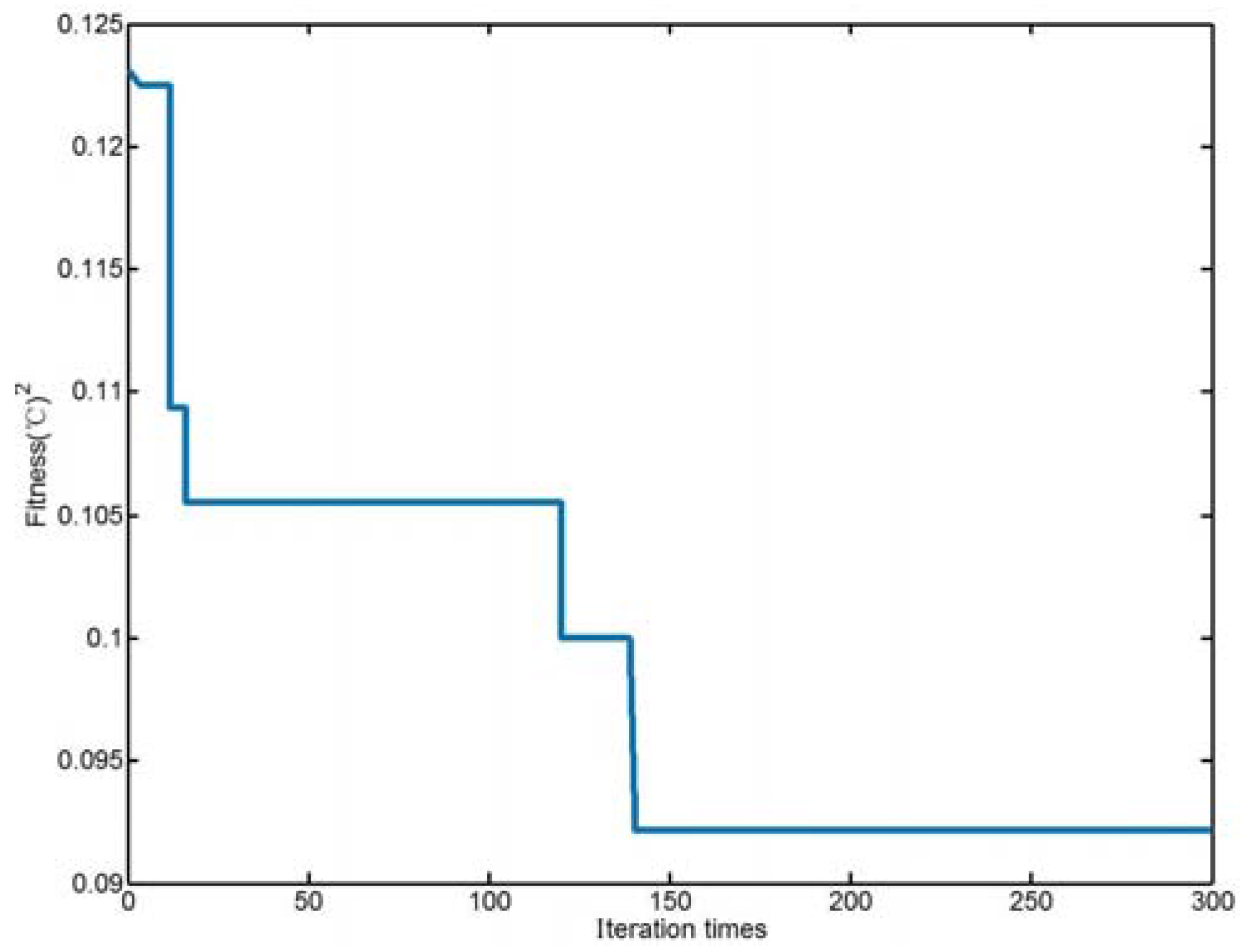
When the temperature of the high-speed output shaft of the gearbox is predicted, in order to optimize the parameters of LSSVM, Y and are considered as two particles, , . Particle number m is 20. The maximum number of iterations Tmax is 300. The range of inertia weight coefficient ω is chosen as [0.4, 0.9]. The formula of the objective function is: . is the predicted temperature. y(t) is the actual temperature. n is sample number.
Through simulation, when c1 and c2 are, respectively, 1.5 and 1.7, the optimized parameters are Y = 65.6085, = 5.9767. Figure 2 is the change of fitness curve during optimization.
In this paper, 10% training samples are deleted each time. 600 sets of data are for training. 400 sets of data are for testing.
3.3. Comparative Analysis of Prediction Results
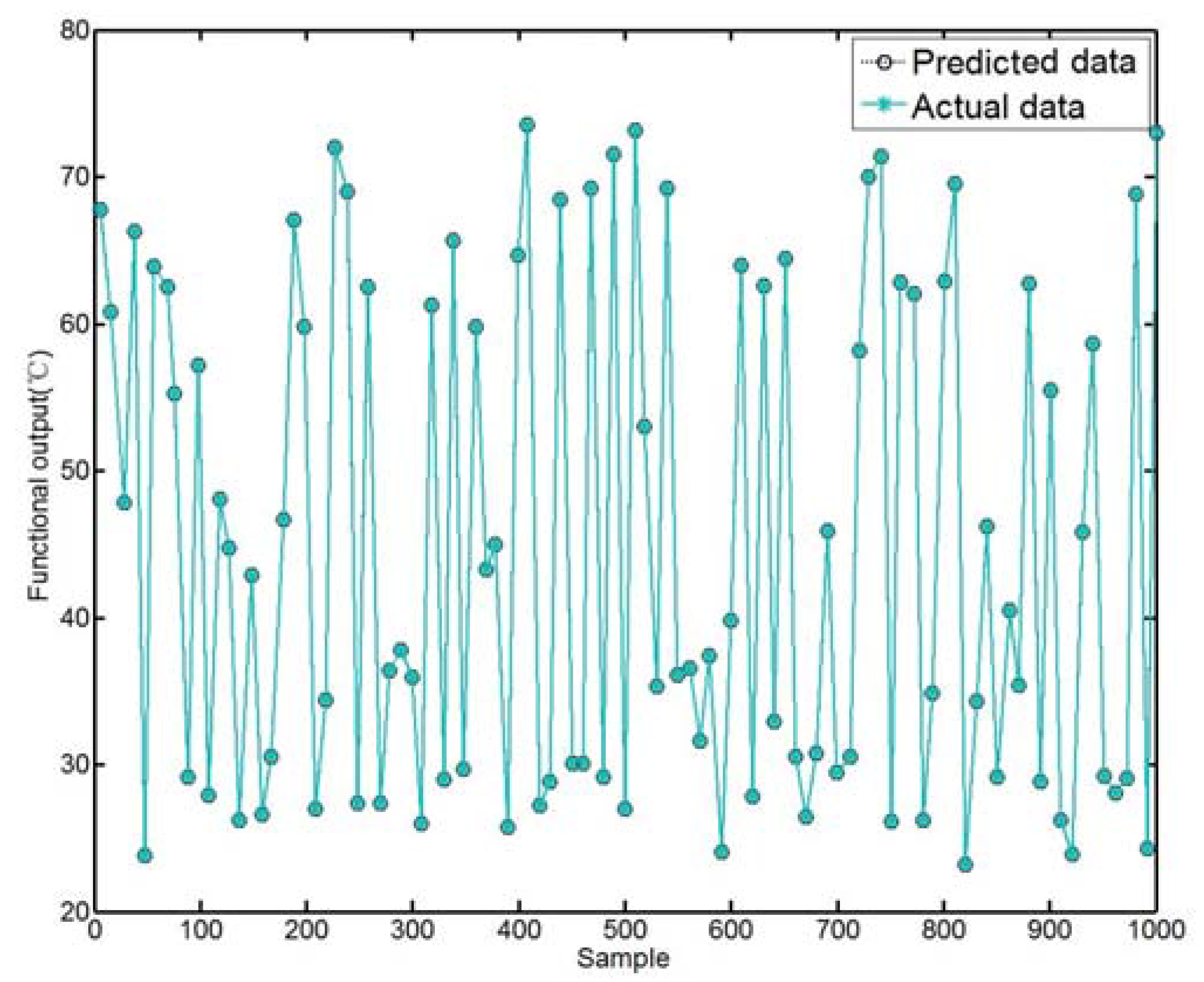
The comparison between the actual data and the predicted data using the proposed pruning PSO-LSSVM model is shown in Figure 3. In order to illustrate the superiority of the model, several other prediction methods are also used to predict temperature. The comparison results are shown in Table 5.
It can be seen from Table 5, when using the same algorithm, different normalization methods are used to predict the temperature. The results of joint normalization are better than the other three methods. For different algorithms, it is obvious that the prediction accuracy of pruning PSO-LSSVM (joint normalization), as proposed by this paper, is the highest, and the prediction time is the shortest. For testing data, the running time is 2.124 s, the correct rate of error within ±5 °C is about 90%, the correct rate of error within ±10 °C is about 93%, the MAPE is 3.7%, and the MSE is 3.8%. The speeds and accuracy of the other algorithms are worse than that of the proposed algorithm. The superiority of the proposed model is proved.
4. Conclusions
In this paper, a pruning algorithm improved LSSVM model is put forward. The temperature of the high-speed output shaft of gearbox is predicted. Joint normalization is used to consider the characteristic of the same and different parameters. In order to reduce the correlation and redundancy of the data, PCA is adopted. In order to reduce the blindness of parameter selection, the PSO algorithm is used to optimize the parameters in the model. The experimental results show that the proposed method has shorter training time and higher prediction accuracy than other methods. It is valuable in real-time forecasting.
Acknowledgments
This work was supported by the National Natural Science Foundation of China (51577008) and the China Scholarship Council. The authors are grateful to the anonymous reviewers for their constructive comments on the paper.
Author Contributions
Yancai Xiao and Ruolan Dai contributed to paper writing and the whole revision process. Guangjian Zhang contributed to paper writing and did the simulation. Weijia Chen helped organize the article. All the authors have read and approved the final manuscript.
Conflicts of Interest
The authors declare no conflicts of interest.
References
- Xiao, Y.; Wang, Y.; Mu, H.; Kang, N. Research on misalignment fault isolation of wind turbines based on the mixed-domain features. Algorithms 2017, 10, 67. [Google Scholar] [CrossRef]
- Xiao, Y.; Kang, N.; Hong, Y.; Zhang, G. Misalignment fault diagnosis of DFWT based on IEMD energy entropy and PSO-SVM. Entropy 2017, 19, 6. [Google Scholar] [CrossRef]
- Crabtree, C.J.; Feng, Y.; Tavner, P.J. Detecting incipient wind turbine gearbox failure: A signal analysis method for on-line condition monitoring. In Proceedings of the European Wind Energy Conference, Warsaw, Poland, 20–23 April 2010. [Google Scholar]
- Guo, P.; Bai, N. Wind turbine gearbox condition monitoring with AAKR and moving window statistic methods. Energies 2011, 4, 2077–2093. [Google Scholar] [CrossRef]
- Kostandyan, E.E.; Sørensen, J.D. Reliability assessment of solder joints in power electronic modules by crack damage model for wind turbine applications. Energies 2011, 4, 2236–2248. [Google Scholar] [CrossRef]
- Liu, Z.; Zhang, P.; Shen, Y. Thermal analysis model of high speed cylindrical roller bearing. Mech. Sci. Technol. 2000, 16, 607–611. [Google Scholar]
- Zhang, J.; Li, Y. Selection and simulation of input variables in the temperature prediction of wind turbine gearbox. J. Xi’an Technol. Univ. 2015, 4, 340–344. [Google Scholar]
- Kusiak, A.; Verma, A. Analyzing bearing faults in wind turbines: A data-mining approach. Renew. Energy 2012, 48, 110–116. [Google Scholar] [CrossRef]
- Schlechtingen, M.; Santos, I.F. Comparative analysis of neural network and regression based condition monitoring approaches for wind turbine fault detection. Mech. Syst. Signal Process. 2011, 25, 1849–1875. [Google Scholar] [CrossRef] [Green Version]
- Guo, P.; David, I.; Yang, X. Wind turbine gearbox condition monitoring using temperature trend analysis. Chin. J. Electr. Eng. 2011, 31, 129–136. [Google Scholar]
- Guo, P.; Infield, D.; Yang, X.Y. Wind turbine generator condition-monitoring using temperature trend analysis. IEEE Trans. Sustain. Energy 2012, 3, 124–133. [Google Scholar] [CrossRef]
- Wang, Z.; Guo, P. Wind turbine spindle condition monitoring based on operational data. In Proceedings of the 29th Chinese Control and Decision Conference, Chongqing, China, 28–30 May 2017; pp. 1435–1440. [Google Scholar]
- Zhang, X.; Yan, S.; Zhou, X.; Zhao, H. Early fault prediction method for main bearing of wind turbine based on state monitoring. Guangdong Power 2012, 11, 7–50. [Google Scholar]
- Zhao, H.; Zhang, X. Early fault prediction of wind turbine gearbox based on temperature measurement. In Proceedings of the 2012 IEEE International Conference on Power System Technology, Auckland, New Zealand, 30 October–2 November 2012; p. 5. [Google Scholar]
- Shin, J.; Lee, Y.; Kim, J. Fault prediction of wind turbine by using the SVM method. In Proceedings of the 2014 International Conference on Information Science, Electronics and Electrical Engineering, Sapporo, Japan, 26–28 April 2014; pp. 1923–1926. [Google Scholar]
- Fang, R.; Jiang, S.; Shang, Y.; Wang, L. On line assessment of the wind turbine gearbox state using the trend state analysis. J. Huaqiao Univ. 2016, 37, 32–37. [Google Scholar]
- Li, H.; Li, X.; Hu, Y.; Yang, C.; Zhao, B. Unequal interval grey prediction of wind turbine operation state parameters. Power Syst. Autom. 2012, 36, 29–34. [Google Scholar]
- He, F.; Zhou, C.; Liu, C. Application of BP neural network in predicting solar greenhouse soil temperature. Int. Agric. Eng. J. 2016, 25, 175–183. [Google Scholar]
- Ma, Z.; Zhao, Z.; Huang, W. Stepwise regression analysis of the melting point of the coal ash in Ruqigou. Coal Geol. China 2010, 22, 7–9. [Google Scholar]
- Xu, J.; Liu, X.; Li, D.; Zhou, Z.; Wang, F.; Yu, G. Study on temperature prediction model of coal ash flow. J. Fuel Chem. 2012, 40, 1415–1421. [Google Scholar]
- Niu, M.; Sun, Y.; Lin, B. Study on calculation formula of coal ash melting temperature. Coal Qual. Technol. 2011, 17, 69–72. [Google Scholar]
- Xu, Z.; Zheng, J.; Wen, X. Prediction of ash fusion point based on partial least squares regression. J. Power Eng. 2010, 30, 788–792. [Google Scholar]
- Zhang, Y.; Yin, Y.; Wang, X. Model for predicting ash melting point of coal ash composition. Sized Nitrogenous Fertil. Prog. 2012, 6, 10–12. [Google Scholar]
- Li, J.; Shen, B.; Li, H.; Zhao, J.; Wang, J. Effect of coal blending on the melting point of coal ash and the prediction model of ash melting point. Coal Qual. Technol. 2009, 5, 66–70. [Google Scholar]
- Kahramanac, H.; Bos, F.; Reifenstein, A. Application of a new ash fusion test to theodore coals. Fuel 1998, 77, 1005–1011. [Google Scholar] [CrossRef]
- Zhang, D.; Long, Y.; Gao, J.; Zhang, B. The relationship between chemical composition of coal ash and ash fusibility. J. East China Univ. Sci. Technol. 2003, 29, 590–594. [Google Scholar]
- Fan, Q.; Pan, P. Analysis of correlation between chemical composition and melting temperature and melting temperature. Boil. Technol. 2007, 38, 10–13. [Google Scholar]
- Cao, X.; Li, H.; Liu, J.; Zhang, Z.; Zhu, B.; Zhao, Q. Effect of mineral concentrate on the melting characteristics of coal ash and its melting mechanism. J. Coal Sci. 2013, 38, 314–319. [Google Scholar]
- Ren, H.; Lei, X.; Zhang, P. A study of wind speed prediction based on particle swarm algorithm to optimize the parameters of sparse least squares support vector. Int. J. Simul. 2016, 17, 1.1–1.7. [Google Scholar]
- Ye, M.; Wang, X.; Zhang, H. Chaotic time series prediction based on online least squares support vector regression. Phys. J. 2005, 54, 2568–2573. [Google Scholar]
- Hemmati-Sarapardeh, A.; Varamesh, A.; Husein, M.M.; Karan, K. On the evaluation of the viscosity of nanofluid systems: Modeling and data assessment. Renew. Sustain. Energy Rev. 2018, 81, 313–329. [Google Scholar] [CrossRef]
- Ahmadi, M.A.; Rozyn, J.; Lee, M.; Bahadori, A. Estimation of the silica solubility in the superheated steam using LSSVM modeling approach. Environ. Prog. Sustain. Energy 2016, 35, 596–602. [Google Scholar] [CrossRef]
- Liu, C.; Niu, P.; Li, G.; You, X.; Ma, Y.; Zhang, W. A hybrid heat rate forecasting model using optimized LSSVM based on improved GSA. Neural Process. Lett. 2017, 45, 299–318. [Google Scholar] [CrossRef]
- Yi, L.; Niu, D.; Ye, M.; Hong, W. Short-term load forecasting based on wavelet transform and least squares support vector machine optimized by improved cuckoo search. Energies 2016, 9, 827. [Google Scholar] [CrossRef]
- Yang, J.; Cheng, Y.; Huang, J. A novel short-term multi-input-multi-output prediction model of wind speed and wind power with LSSVM based on quantum-behaved particle swarm optimization algorithm. Chem. Eng. Trans. 2017, 59, 871–876. [Google Scholar]
- Liu, X. Research on normalization of input layer data of BP neural network. Mechan. Eng. Autom. 2010, 3, 123–126. [Google Scholar]
- Santos-Alamillos, F.J.; Thomaidis, N.S.; Quesada-Ruiz, S.; Ruiz-Arias, J.A.; Pozo-Vázquez, D. Do current wind farms in Spain take maximum advantage of spatiotemporal balancing of the wind resource. Renew. Energy 2016, 96, 574–582. [Google Scholar] [CrossRef]
- Zhang, W.; Ma, D.; Wei, J.J.; Liang, H. A parameter selection strategy for particle swarm optimization based on particle positions. Expert Syst. Appl. 2014, 41, 3576–3584. [Google Scholar] [CrossRef]
- Pousinho, H.M.I.; Catalao, J.P.S.; Mendes, V.M.F. Wind power short-term prediction by a hybrid PSO-ANFIS approach. In Proceedings of the Melecon 2010–2010 15th IEEE Mediterranean Electrotechnical Conference, Valletta, Malta, 25–28 April 2010; pp. 955–960. [Google Scholar]
- Sun, P.; Li, J.; Chen, J.; Lei, X. A short-term outage model of wind turbines with doubly fed induction generators based on supervisory control and data acquisition data. Energies 2016, 9, 882. [Google Scholar] [CrossRef]
Figure 1.
Schematic of the model.
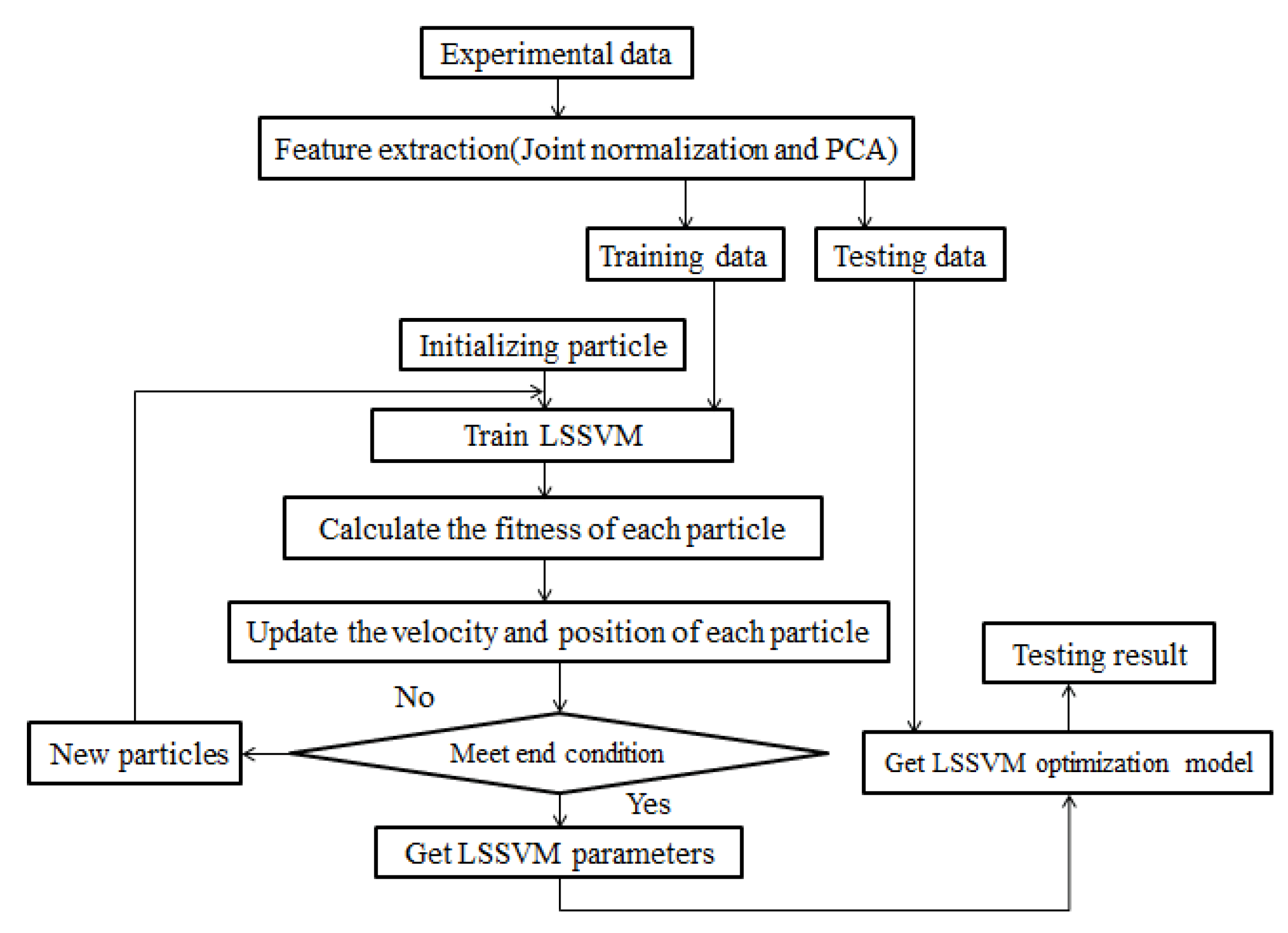
Figure 2.
Particle swarm optimization (PSO) fitness curve.

Figure 3.
Predicted data of the proposed model compared with the actual data.

Table 1.
Comparison of temperature prediction methods.
| Method | Characteristic | Advantages | Disadvantages |
|---|---|---|---|
| BP neural network | It is a nonlinear regression method, which has strong nonlinear mapping ability [18]. | The adaptability is strong. The forecasting precision is high, and the modeling process is more convenient and direct. It is not necessary to specify the direct relationship between input and output. | It requires huge data samples. Less samples cannot get accurate results. |
| Nonlinear state estimation | A method for estimating the internal state of a dynamic system based on measured data. | Non parametric modeling method. Clear physical meaning. | Low accuracy. Poor implementation. |
| Linear regression method | The curve is fitted by using various algorithms, including stepwise regression method [19,20,21,22], piecewise fitting method [23,24], regression analysis fitting [25], partial least squares regression [26,27], least squares regression [28]. | Operation is more convenient. | The adaptability of the prediction model is poor, only in the proper scope it has a good prediction effect. |
| Support vector machine | It has many unique advantages in solving a few, nonlinear and high dimensional samples. | The prediction precision is high and the samples are relatively a few. | The choice of parameters affects the accuracy of the model. |
| Gray model | Based on the generated data, but not the original data. | Do not need a lot of samples. There is small amount calculation. | It is better for predicting data with definite trends. |
Table 2.
Part of original sample data.
| Nacelle Vibration x (mm) | Nacelle Vibration y (mm) | Wind Speed (m/s) | Rotor Speed (r/min) | Gearbox Tempera-Ture Input Shaft (°C) | Gearbox Tempera-Ture Output Shaft (°C) | Gearbox Oil Tempera-Ture (°C) | Grid Power (KW) | Main Bearing Gearbox Side Temperature (°C) |
|---|---|---|---|---|---|---|---|---|
| −0.00779748 | −0.002426243 | 9.285114 | 12.84335 | 62.9 | 64.9 | 56.8 | 316.8 | 40.5 |
| −0.004867697 | 0.007827997 | 9.329819 | 12.84534 | 62.1 | 64 | 55.8 | 318.6 | 40.3 |
| −0.001937914 | −0.000473023 | 9.821562 | 12.92032 | 61.2 | 63.3 | 55 | 316.8 | 40.1 |
| −0.000961351 | 0.004898214 | 8.916306 | 12.98766 | 60.3 | 62.7 | 54.6 | 316.8 | 39.9 |
| −0.000961351 | −0.003402805 | 10.03391 | 13.04737 | 59.6 | 62.1 | 54.1 | 315.6 | 39.7 |
| −0.003891087 | 0.00148015 | 11.45326 | 12.95979 | 59.1 | 61.6 | 53.6 | 314.4 | 39.5 |
| −0.002914524 | −0.002914524 | 8.234571 | 13.04737 | 58.7 | 61.1 | 53 | 316.2 | 39.4 |
| −0.001937914 | 0.008316278 | 11.17386 | 13.01453 | 58.5 | 60.6 | 51.8 | 315.6 | 39.3 |
| 0.00050354 | −0.007309198 | 11.49796 | 12.9369 | 58.6 | 60.1 | 50.3 | 319.2 | 39.1 |
| −0.000473023 | −0.001937914 | 11.59855 | 13.09713 | 59.4 | 61.2 | 53.6 | 325.2 | 39 |
Table 3.
Part of data after joint normalization.
| Nacelle Vibration x | Nacelle Vibration y | Wind Speed | Rotor Speed | Gearbox Tempera-Ture Input Shaft | Gearbox Tempera-Ture Output Shaft | Gearbox Oil Tempera-Ture | Grid Power | Main Bearing Gearbox Side Tempera-Ture |
|---|---|---|---|---|---|---|---|---|
| 0.282 | 0.049 | 0.601 | 0.469 | 0.55 | 0.491 | 0.510 | 0.591 | 0.898 |
| 0.128 | 0.575 | 0.608 | 0.469 | 0.505 | 0.448 | 0.439 | 0.589 | 0.864 |
| 0.02 | 0.150 | 0.693 | 0.478 | 0.455 | 0.414 | 0.382 | 0.591 | 0.830 |
| 0.025 | 0.425 | 0.537 | 0.486 | 0.405 | 0.386 | 0.354 | 0.591 | 0.796 |
| 0.076 | 1.279 | 0.730 | 0.492 | 0.366 | 0.357 | 0.319 | 0.593 | 0.762 |
| 0.076 | 0.250 | 0.974 | 0.482 | 0.338 | 0.333 | 0.283 | 0.594 | 0.728 |
| 0.076 | 0.025 | 0.419 | 0.492 | 0.316 | 0.309 | 0.241 | 0.592 | 0.711 |
| 0.025 | 0.599 | 0.926 | 0.489 | 0.305 | 0.285 | 0.156 | 0.593 | 0.694 |
| 0.025 | 0.199 | 0.982 | 0.480 | 0.311 | 0.261 | 0.049 | 0.588 | 0.661 |
| 0.153 | 0.075 | 1 | 0.498 | 0.355 | 0.314 | 0.283 | 0.580 | 0.644 |
Table 4.
Principal components and their contribution rate.
| Serial Number | Characteristic Value | Contribution Rate | Cumulative Contribution Rate |
|---|---|---|---|
| 1 | 4.938 | 54.861% | 54.861% |
| 2 | 1.350 | 15.004% | 69.865% |
| 3 | 1.198 | 13.312% | 83.178% |
| 4 | 0.681 | 7.563% | 90.740% |
| 5 | 0.617 | 6.859% | 97.599% |
| 6 | 0.186 | 2.065% | 99.664% |
| 7 | 0.016 | 0.178% | 99.841% |
| 8 | 0.010 | 0.116% | 99.957% |
| 9 | 0.004 | 0.116% | 100% |
Table 5.
Comparison of various algorithm results.
| Method | Time(s) | t-Test | Accuracy of Error within ±5 °C | Accuracy of Error within ±10 °C | Mean Absolute Percentage Error (MAPE) | Mean Squared Error (MSE) |
|---|---|---|---|---|---|---|
| LSSVM (normalized with maximum-minimum method) | 4.958 | 0.0037 | 75% | 78% | 7.3% | 7.6% |
| LSSVM (normalized with peak method) | 4.957 | 0.0045 | 76% | 79% | 7.4% | 7.5% |
| LSSVM (normalized with value method) | 4.976 | 0.0054 | 78% | 80% | 7.2% | 7.1% |
| LSSVM (joint normalization) | 3.675 | 0.0056 | 80% | 82% | 6.5% | 6.8% |
| PCA-LSSVM (normalized with maximum-minimum method) | 3.567 | 0.0067 | 78% | 79% | 6.5% | 6.5% |
| PCA-LSSVM (normalized with peak method) | 3.987 | 0.0034 | 79% | 80% | 6.4% | 6.4% |
| PCA-LSSVM (normalized with value method) | 3.765 | 0.0045 | 81% | 82% | 6.3% | 6.2% |
| PCA-LSSVM (joint normalization) | 2.345 | 0.0056 | 83% | 84% | 5.6% | 5.8% |
| PSO-PCA-LSSVM (normalized with maximum-minimum method) | 3.125 | 0.0034 | 81% | 84% | 5.6% | 5.7% |
| PSO-PCA-LSSVM (normalized with peak method) | 3.135 | 0.0065 | 83% | 86% | 5.4% | 5.9% |
| PSO-PCA-LSSVM (normalized with value method) | 3.173 | 0.0075 | 82% | 85% | 5.2% | 5.1% |
| PSO-PCA-LSSVM (joint normalization) | 2.473 | 0.0064 | 85% | 87% | 4.7% | 4.9% |
| Pruning PSO-PCA-LSSVM (normalized with maximum-minimum method) | 2.348 | 0.0036 | 84% | 91% | 4.6% | 4.4% |
| Pruning PSO-PCA-LSSVM (normalized with peak method) | 2.475 | 0.0065 | 83% | 92% | 4.7% | 4.5% |
| Pruning PSO-PCA-LSSVM (normalized with value method) | 2.725 | 0.0076 | 85% | 92% | 4.3% | 4.2% |
| Pruning PSO-PCA-LSSVM (joint normalization) | 2.124 | 0.0045 | 90% | 93% | 3.7% | 3.8% |
| SVM | 6.453 | 0.1576 | 70% | 85% | 5.8% | 8.9% |
© 2017 by the authors. Licensee MDPI, Basel, Switzerland. This article is an open access article distributed under the terms and conditions of the Creative Commons Attribution (CC BY) license (http://creativecommons.org/licenses/by/4.0/).
Share and Cite
MDPI and ACS Style
Xiao, Y.; Dai, R.; Zhang, G.; Chen, W. The Use of an Improved LSSVM and Joint Normalization on Temperature Prediction of Gearbox Output Shaft in DFWT. Energies 2017, 10, 1877. https://doi.org/10.3390/en10111877
AMA Style
Xiao Y, Dai R, Zhang G, Chen W. The Use of an Improved LSSVM and Joint Normalization on Temperature Prediction of Gearbox Output Shaft in DFWT. Energies. 2017; 10(11):1877. https://doi.org/10.3390/en10111877
Chicago/Turabian StyleXiao, Yancai, Ruolan Dai, Guangjian Zhang, and Weijia Chen. 2017. "The Use of an Improved LSSVM and Joint Normalization on Temperature Prediction of Gearbox Output Shaft in DFWT" Energies 10, no. 11: 1877. https://doi.org/10.3390/en10111877
Note that from the first issue of 2016, this journal uses article numbers instead of page numbers. See further details here.