1. Introduction
The system frequency of an electric grid should be kept within an allowable range at all times to ensure stable operation. To achieve this goal, if a large frequency event such as a generator tripping occurs, the decreased frequency should be promptly recovered to the nominal value. In a conventional electric power grid, synchronous generators that have spinning reserve increase their mechanical power by relying on the frequency deviation [
1]. The frequency nadir is an important metric in maintaining the frequency stability.
For an electric power grid that has a high level of wind power penetration, variable-speed wind turbine generators (WTGs)—e.g., doubly-fed induction generator (DFIG)-based WTGs and full converter-based WTGs—perform a maximum power point tracking (MPPT) operation that extracts the maximum energy from the wind at different wind speeds [
2,
3]. However, this operation adversely impacts frequency stability [
4,
5]. Therefore, some countries specify requirements on the frequency response of WTGs [
6,
7], and a number of studies on the frequency response of WTGs have been reported in the literature [
8,
9,
10,
11,
12,
13,
14,
15,
16].
The frequency-supporting capabilities of a WTG can be classified into two groups: short-term frequency response (STFR) [
8,
9,
10,
11,
12,
13,
14] and long-term frequency response [
15,
16]. The former temporarily releases the kinetic energy stored in the rotating masses in a WTG without the reserve power. In contrast, the latter releases the reserve power to compensate for part of the deficient power. Thus, the latter provides more contribution to frequency response; however, the latter requires the deloaded operation of a WTG, and this inevitably causes a significant loss of annual energy. Thus, this paper focuses on the STFR of a WTG and assumes that a WTG operates in an MPPT mode prior to a disturbance.
STFR schemes have been reported that release kinetic energy depending on the system frequency [
8,
9]; however, these schemes provide a slow response. To provide a faster response, STFR schemes were suggested that promptly increase the output power when an event is detected [
10,
11,
12,
13,
14]. The power reference, which is defined as a function of time, increases the output, and this value is maintained for a preset period. Then, to recover the rotor speed, the power reference in [
10,
11] is abruptly reduced to a preset value and the reference for MPPT operation, respectively. The scheme in [
11] can recover the rotor speed faster than the scheme in [
10], but it causes a large second frequency drop (SFD). In addition, to ensure the stable operation of a WTG, the schemes in [
10,
11] should increase the power reference by a small value only. On the contrary, the schemes in [
12,
13,
14] can release more kinetic energy while preventing over-deceleration because the power reference is defined as a function of the rotor speed. When an event is detected, the schemes in [
12,
13] simply add a constant to the reference for MPPT. In contrast, the scheme in [
14] increases the reference to the torque limit referred to power, thereby improving the frequency nadir higher than those in [
12,
13]; then, the reference is linearly reduced with the rotor speed. To recover the rotor speed, the schemes in [
12,
13,
14] reduce the reference by a small value after the rotor speed is converged to a value in the stable region; then, the reference is maintained until the reference reaches the reference for MPPT. Thus, the schemes in [
12,
13,
14] can ensure a small SFD; however, the slow rotor speed is inevitable for a higher rotor speed, thereby delaying the frequency stabilization.
This paper proposes an STFR scheme of a DFIG-based WTG that ensures fast frequency stabilization while improving the frequency nadir. To achieve these objectives, the power reference function is defined in four stages. Stage I and Stage II belong to the energy-releasing period, while Stage III and Stage IV are in the energy-absorbing period. In the energy-releasing period, to speed up the rotor speed convergence while improving the frequency nadir, at Stage I, the power reference is increased up to the torque limit referred to power and reduced along with the torque limit referred to power for a predefined period. At Stage II, to converge the rotor speed into the stable operating region, the power reference decreases linearly with the rotor speed. In the energy-absorbing period, to promptly recover the rotor speed, at Stage III, the power reference smoothly decreases with the rotor speed and time during a predefined period so that it meets the reference for MPPT. At Stage IV, the rotor speed is eventually recovered to the value prior to an event along with the MPPT curve. The efficacy of the proposed scheme is verified with various wind conditions based on the IEEE 14-bus system using an electromagnetic transient program restructured version (EMTP-RV) simulator, which is a technically advanced simulation and analysis software for power system transients.
2. Modeling and Control of a DFIG-Based WTG
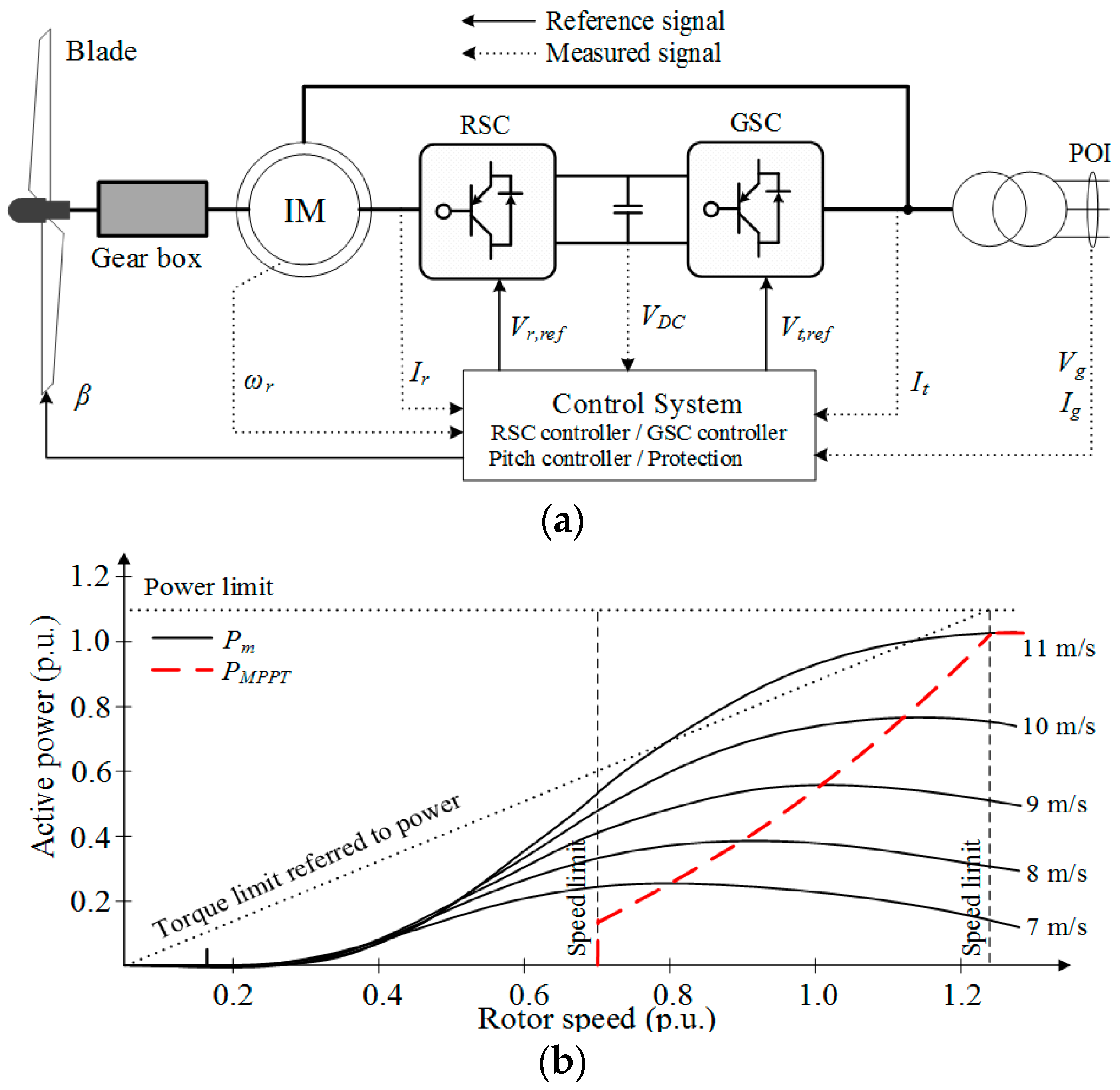
Figure 1a depicts a typical configuration of a DFIG-based WTG model: a wind turbine model, an induction machine, and a control system.
As in [
17], the mechanical power extracted from the wind,
Pm, is given by:
where
ρ is the air density in kg/m
3,
A is the rotor-swept area of a DFIG-based WTG in m
2,
vwind is the wind speed in m/s, and
cP is the power coefficient, which is a function of tip-speed ratio,
λ and pitch angle,
β.
The references for a rotor-side convertor (RSC) and grid-side convertor (GSC) are determined by a DFIG-based WTG control system. The RSC controls the active and reactive powers supplied into an electric power grid; whereas the GSC maintains the DC-link voltage [
18,
19].
As in [
20], to extract the maximum energy from the wind, the reference for MPPT operation,
PMPPT, is set to:
Table 1 shows the parameters of a DFIG-based WTG used in this study.
Figure 1b illustrates
PMPPT and the mechanical power curves at different wind speeds as indicated by a red dashed line and the black solid lines, respectively. To obtain realistic results, this paper considers the power limit and torque limit referred to power as represented by the two black dotted lines. In this paper, the maximum power and torque limits of the DFIG-based WTG are set to 1.10 p.u. and 1.07 p.u., respectively; the rate limit is set to 0.45 p.u./s [
21]. The operating range of the rotor speed is from 0.70 p.u. (
ωmin) to 1.25 p.u. (
ωmax). In addition, when the rotor speed reaches 1.25 p.u., the pitch controller is activated.
3. STFR Schemes of a DFIG-Based WTG
In this section, the overall operational features of the two conventional schemes in [
10,
14], which are represented as Scheme #1 and Scheme #2, respectively, in this paper, are briefly described. Then, the operational characteristics of the proposed scheme are described.
3.1. Scheme #1
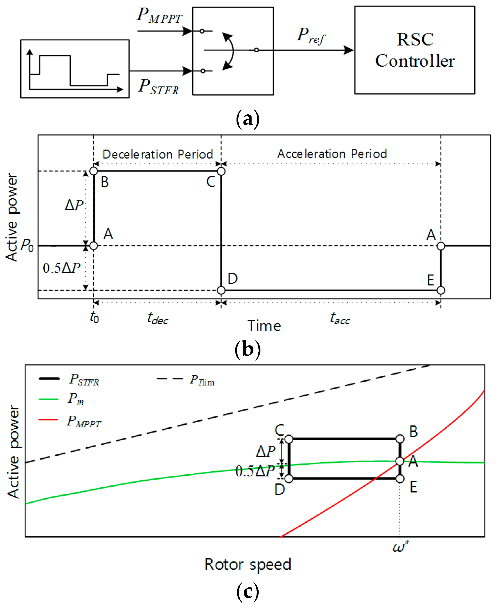
Figure 2a illustrates the control scheme of Scheme #1 [
10]. At the instant of a frequency event, Scheme #1 switches the power reference,
Pref, from
PMPPT to
PSTFR, which is defined in the time domain. At
t0,
Pref instantly increases from
P0 to
P0 + Δ
P. At
t0 +
tdec,
Pref abruptly decreases from
P0 + Δ
P to
P0 − 0.5Δ
P. At
t0 +
tdec +
tacc,
Pref is returned to
PMPPT.
Pref at Point D should be smaller than
Pm so that
ωr starts recovering (see
Figure 2c). To prevent over-deceleration, a small Δ
P should be determined and it was set to 0.1 p.u.;
tdec and
tacc are set to 10.0 s and 20.0 s, respectively [
10]. At
t0 +
tdec, to restore the
ωr, 0.15 p.u. is abruptly reduced.
3.2. Scheme #2
In Scheme #2 [
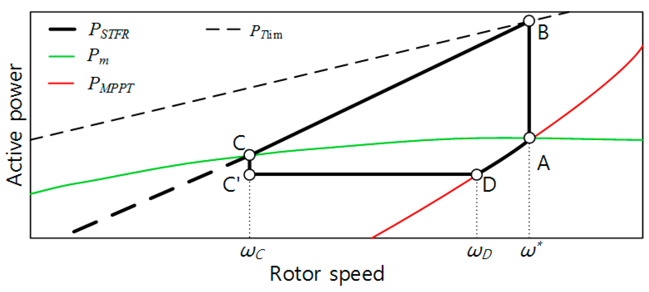
14], to improve the frequency nadir while ensuring stable operation,
Pref is defined as a function of
ωr, as shown in
Figure 3. Upon detecting an event, Scheme #2 increases
Pref from
P0 to
PTlim(
ω*), which is the torque limit referred to power at
ω*. Thus, Scheme #2 is capable of improving the frequency nadir than that in Scheme #1 by releasing more kinetic energy.
Then, to converge
ωr to a point in the stable region,
Pref is reduced as a function of
ωr (from Point B to Point C in
Figure 3) as in
where
PMPPT(
ωmin) is
PMPPT at
ωmin.
During this period, ωr keeps decreasing until it converges to ωC, which is a point of intersection of (3) and Pm. Note that ωC is determined between ωmin and ω*; this means that ωC is located in the stable region, and thus Scheme #2 ensures stable operation while supporting the frequency.
To recover ωr to ω*, Scheme #2 abruptly reduces Pref at Point C, as Scheme #1 does; however, the reduced power is 0.03 p.u., which is 20% of the reduced power (0.15 p.u.) in Scheme #1. Thus, Scheme #2 causes a significantly smaller SFD than Scheme #1. At ωC, Pref is reduced to Pref(ωC) − 0.03 p.u., which is maintained until Pref meets PMPPT at Point D; thereafter, ωr is returned to ω* along with the PMPPT curve. Therefore, Scheme #2 can improve the frequency nadir at a higher level while ensuring a smaller SFD than Scheme #1. However, for a higher ω*, the ωr recovery becomes significantly slower than that in Scheme #1, thereby delaying the frequency stabilization.
3.3. Proposed STFR Scheme of a DFIG-Based WTG for the Rapid Rotor Speed Recovery
This paper aims to improve the
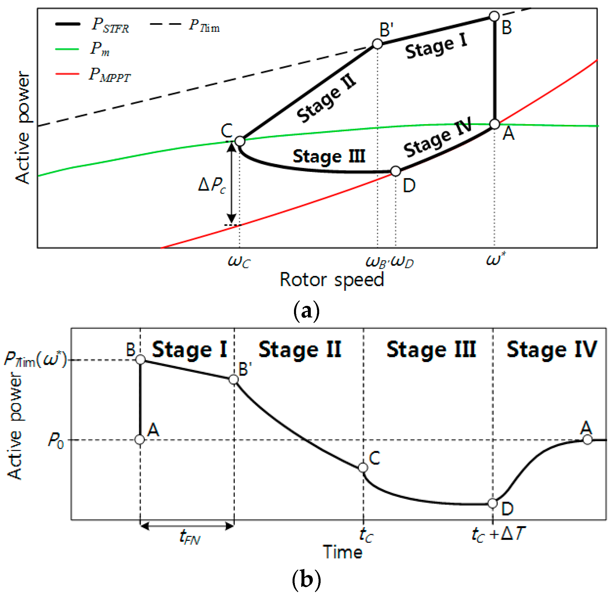
ωr recovery faster than Scheme #2 while improving the frequency nadir at a higher level, thereby providing rapid frequency stabilization. As shown in
Figure 4a, upon detecting an event, the proposed scheme instantly increases
Pref to
PTlim(
ω*) as Scheme #2 does; then,
Pref in the proposed scheme consists of four stages. Stage I and Stage II, in which
ωr keeps decreasing until it converges to
ωC, correspond to the section from Point B to Point C in Scheme #2. Stage III corresponds to the section from Point C to Point D in Scheme #2; finally, Stage IV is the same as the section from Point D to Point A in Scheme #2. During Stage III and Stage IV,
ωr keeps increasing until
ωr reaches
ω*.
3.3.1. Energy-Releasing Period: Stage I and Stage II
To support the frequency, the proposed scheme instantly increases
Pref up to
PTlim(
ω*) upon detecting an event as in Scheme #2. As a result,
ωr decreases. To accelerate the
ωr convergence faster than Scheme #2,
Pref should be larger than that in Scheme #2 because the reduction rate of
ωr depends on the difference between
Pref and
Pm. To do this,
Pref is reduced along with
PTlim(
ωr) for the preset time, which is represented as
tFN in this paper, as in:
In this paper,
tFN is determined in association with the time of occurrence of the frequency nadir in an electric power grid.
Pref in (4) can not only accelerate the reduction in
ωr, but improve the frequency nadir at a higher level than the conventional schemes because the maximum kinetic energy can be released until around the frequency nadir. However, if a WTG has a smaller kinetic energy level under low wind conditions, where
PTlim(
ω*) becomes larger than that under high wind conditions (see
Figure 1b), a large
tFN can cause over-deceleration. To prevent this, in the proposed scheme,
tFN is set to zero if
ω* is equal to or smaller than 0.9 p.u.
At Stage II,
Pref is defined as
Pref in (5) is a straight line, like it is in (3) in Scheme #2. Note that ωC in the proposed scheme can be set to any point in the stable operating region depending on design purposes, while ωC in Scheme #2 is fixed for a ω*. If ωC can be set to a value close to ωB’, a slope between Point B’ and Point C becomes very large, thereby causing an SFD. Thus, careful attention should be paid on selecting ωC so that it can avoid an SFD between Point B’ and Point C. For comparison, ωC in the proposed scheme is set to be the same as that in Scheme #2; this means that in Scheme #2 and the proposed scheme the total released kinetic energy while performing STFR is the same. However, ωr in the proposed scheme converges to ωC faster than that in Scheme #2 because Pref at Stage I and Stage II in the proposed scheme are larger. As a result, the proposed scheme can start recovering ωr earlier than it does in Scheme #2. This helps to rapidly restore ωr to ω*.
It is decided that
ωr converges to
ωC if (6) is satisfied.
3.3.2. Energy-Absorbing Period: Stage III and Stage IV
To recover ωr to ω*, Scheme #1 and Scheme #2 abruptly reduce Pref by 0.15 p.u., and 0.03 p.u., respectively. Thus, Scheme #2 ensures a small SFD, but slows the ωr recovery.
To improve the ωr recovery to ω* faster than Scheme #2, the power reduction at ωC larger than 0.03 p.u. is required. However, the instant power reduction of larger than 0.03 p.u. can cause a larger SFD. To avoid this, the proposed scheme reduces the power smoothly during the preset period of ΔT instead of reducing it instantly.
In this paper,
Pref at Stage III is defined as:
where Δ
PC is
Pref(
ωC) −
PMPPT(
ωC), as shown in
Figure 4a; and Δ
T is the period of Stage III.
PMPPT, which is the first term in (7), is proportional to the cube of
ωr (see (2)) while the second term of (7) is a function of time. Thus,
Pref in (7) smoothly decreases with
ωr and
t. As time goes on,
ωr increases so that
PMPPT increases; in addition, the second term decreases from Δ
PC to zero at
tC + Δ
T (Point D), where
Pref reaches
PMPPT. Note that in the proposed scheme the duration for
ωr recovery can be controlled by setting Δ
T. The use of a small Δ
T leads Point D in
Figure 4a to move to the left, therefore increasing the difference between
Pm at Point C and
Pref at Point D. Thus, a small Δ
T is desirable for the rapid
ωr recovery but can cause a significant SFD; in contrast, the use of a large Δ
T conversely results in the small SFD but slows the
ωr recovery. In this paper, Δ
T is set to 15.0 s by compromising the
ωr recovery duration and size of an SFD.
At Point D, where Stage IV starts, ωr moves to ω* along with PMPPT.
5. Case Studies
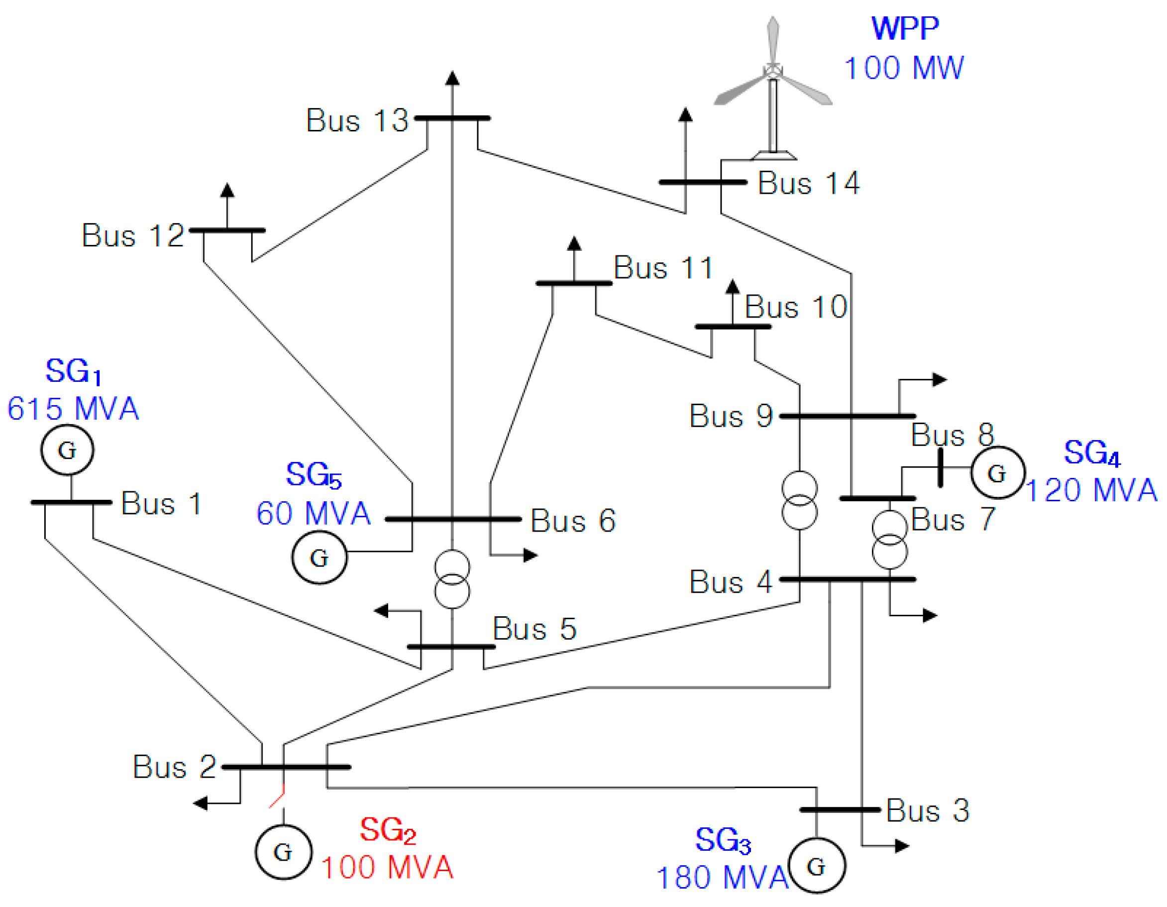
The performance of the STFR schemes of a WTG is affected by the wind speed. Thus, this section investigates the performance of STFR schemes under various wind speeds with the wind power penetration level of 18.6%; this paper defines the wind power penetration level as the installed capacity of a WPP divided by the total load [
24].
Table 3 shows the initial outputs of synchronous generators and the WPP for three cases. As a disturbance, Synchronous Generator 2 (SG
2) generating approximately 100 MW is tripped out at 50.0 s for all cases.
The performance of the proposed STFR scheme is compared to Scheme #1 in [
10] and Scheme #2 in [
14]; in addition, it is compared to MPPT operation. As suggested in [
10],
tdec and
tacc in Scheme #1 are set to 10.0 s and 20.0 s, respectively; Δ
P is set to be 0.1 p.u. The following subsections describe the comparison results of the STFR schemes for three cases.
5.1. Effects of Wind Speeds
The wind speed affects the performance of the STFR schemes of a WTG, thereby resulting in different levels of kinetic energy in a WTG. Thus, this subsection validates the effects of high (10.0 m/s), medium (9.0 m/s), and low (8.0 m/s) speeds on the performance of the STFR schemes.
5.1.1. Case 1: Wind Speed of 10.0 m/s and Wind Power Penetration Level of 18.6%
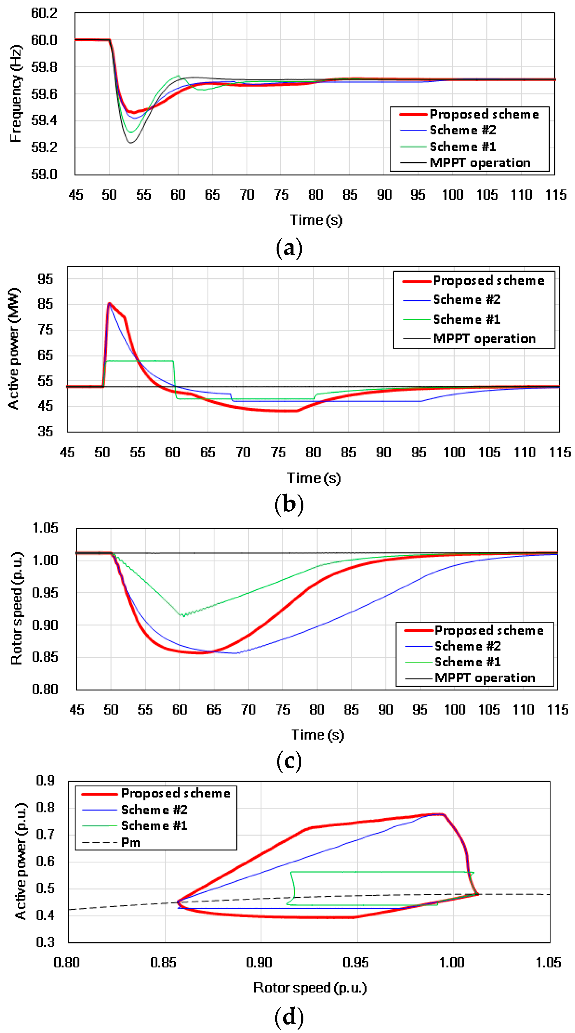
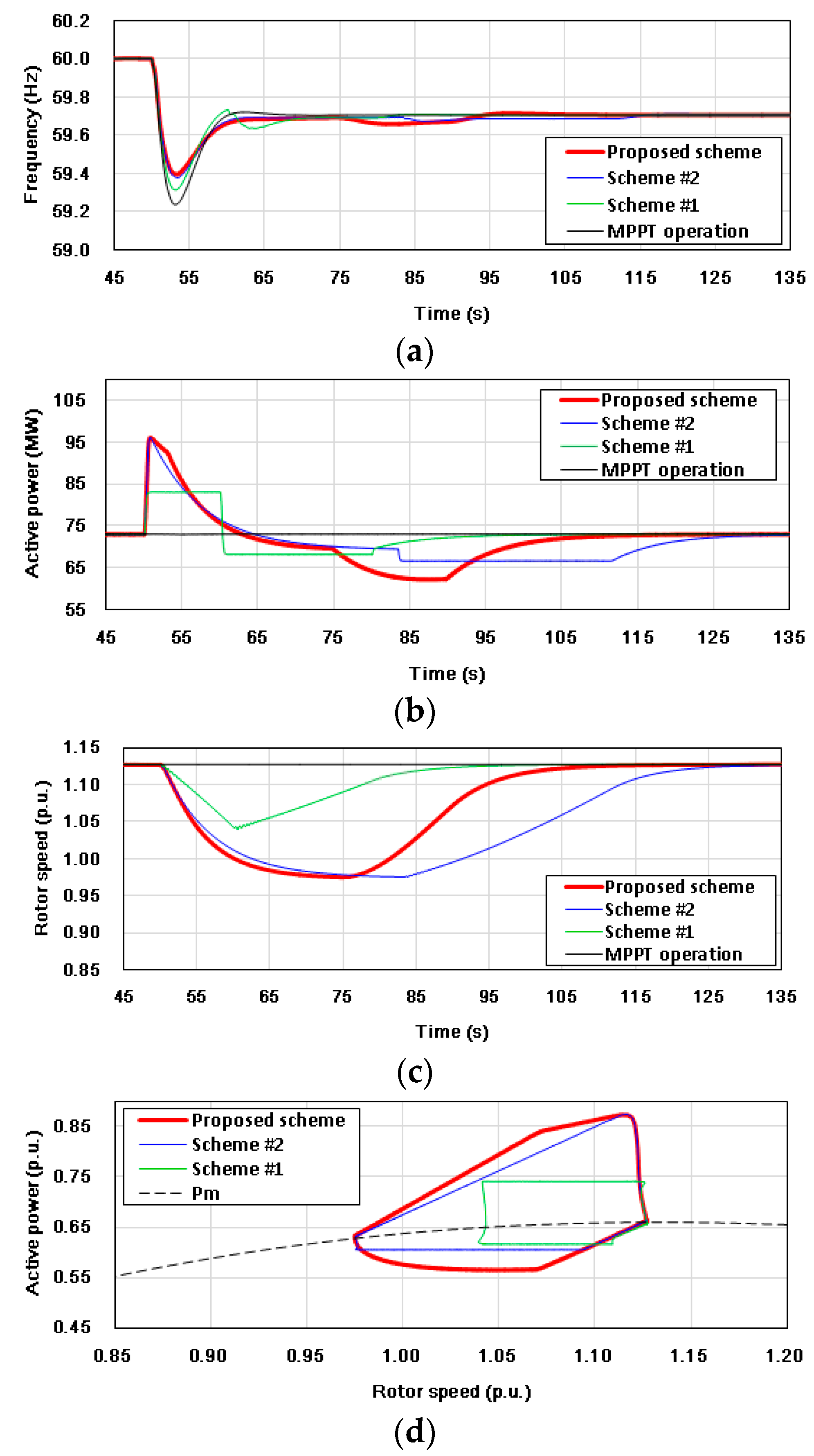
Figure 6 illustrates the results for Case 1. In this case,
tFN is set to 3.0 s because the frequency nadir in the IEEE 14-bus system regularly appears approximately 3.0 s after an event. In addition,
ωC is set to 0.98 p.u.
The frequency nadir in the proposed scheme is 59.40 Hz, which is higher than that in Scheme #2 by 0.02 Hz, and higher than that in Scheme #1 by 0.09 Hz (see
Figure 6a). The frequency nadir for the proposed scheme is higher than those in the conventional schemes because the proposed scheme releases more kinetic energy until around the frequency nadir.
As shown in
Figure 6c,
ωr in the proposed scheme and Scheme #2 converge to the same value of 0.98 p.u. at 75.1 s and 83.5 s, respectively. Note that
ωr in the proposed scheme is converged faster than that in Scheme #2 by 8.4 s because of a larger
Pref in Stage I and Stage II (energy-releasing period) even though both schemes release the same kinetic energy.
For recovering
ωr, 0.15 p.u. is instantly reduced from
Pref in Scheme #1 at 60.0 s, where a significant SFD of 0.098 Hz occurs. (In this study, the size of an SFD is defined as the difference between the frequency prior to an SFD and the second frequency nadir.) In Scheme #2, 0.03 p.u. is instantly reduced from
Pref after
ωr converges at 83.5 s, where a small SFD of 0.021 Hz occurs; however, this results in the slow
ωr recovery, therefore delaying the frequency stabilization. In contrast to the conventional schemes, in the proposed scheme, 0.08 p.u. is smoothly reduced from
Pref for 15.0 s after
ωr converges at 75.1 s. The size of an SFD in the proposed scheme is 0.034 Hz, which is significantly smaller than that in Scheme #1 and slightly larger than in Scheme #2. As shown in
Figure 6c, the duration for
ωr recovery is 64.5 s, which is faster than it is in Scheme #2 by 18.0 s because of the faster
ωr convergence and a larger difference between
Pm and
Pref in Stage III. Consequently, the system frequency in the proposed scheme is stabilized significantly faster than it is in Scheme #2 with a slightly larger SFD (see
Figure 6a).
As shown in
Figure 6d, the proposed scheme increases
Pref up to the torque limit referred to power upon detecting an event and decreases
Pref along with
PTlim for 3.0 s. Afterward,
Pref linearly reduces to
ωC. After the reduction in
Pref,
ωr successfully returns to
ω*.
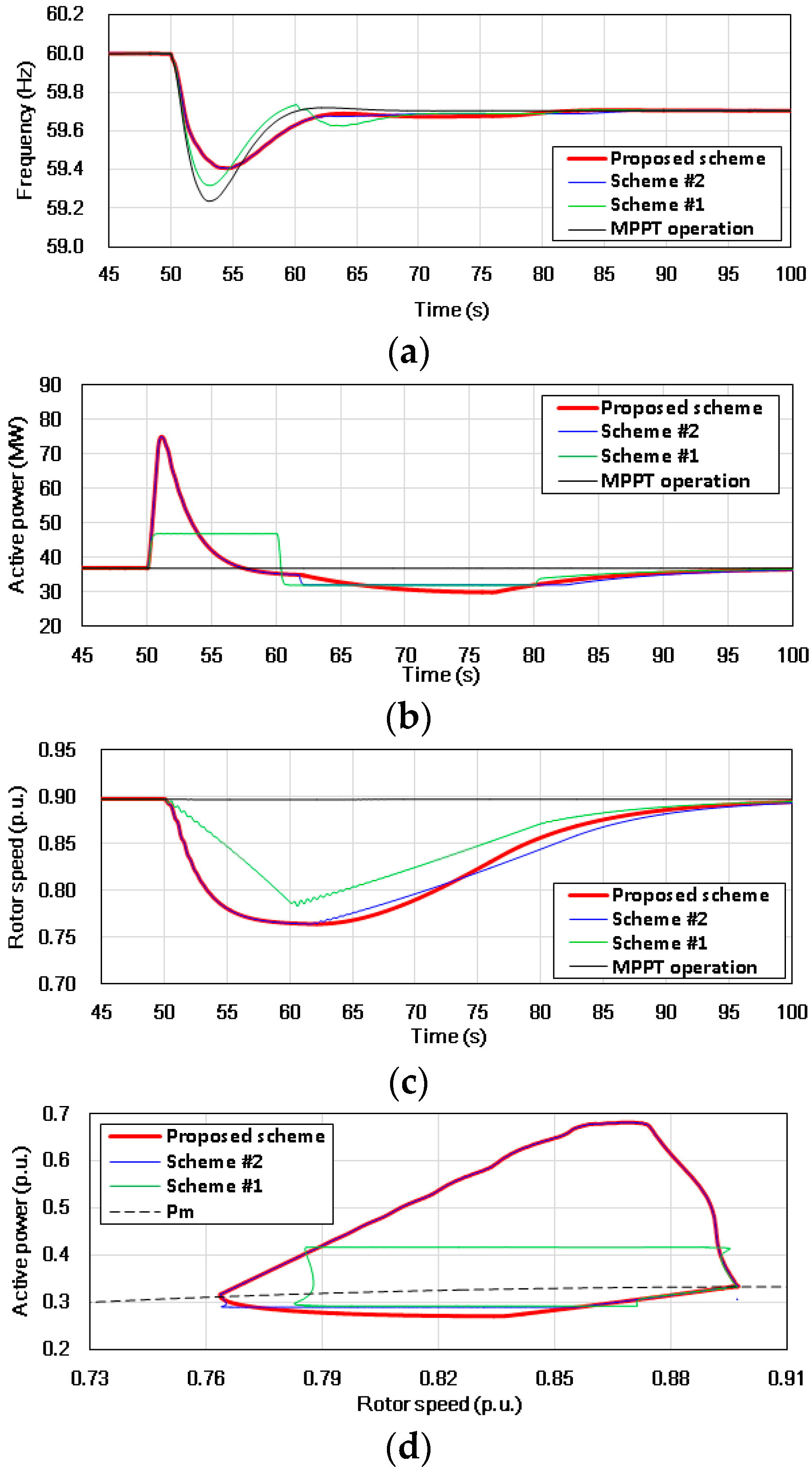
5.1.2. Case 2: Wind Speed of 9.0 m/s and Wind Power Penetration Level of 18.6%
Figure 7 illustrates the results for Case 2. In this case,
tFN is set to 3.0 s and
ωC is set to 0.86 p.u.
The frequency nadir in the proposed scheme is 59.46 Hz, which is higher than that in Scheme #2 by 0.04 Hz, and higher than that in Scheme #1 by 0.15 Hz. This is because the proposed scheme releases a larger kinetic energy than Scheme #1 and Scheme #2 until around the frequency nadir as in Case 1.
As in Case 1,
ωr in the proposed scheme converges to 0.86 p.u. at 63.0 s, which is faster than that in Scheme #2 by 5.3 s because of a larger
Pref in the energy-releasing period. To recover
ωr, Scheme #1 causes a large SFD of 0.101 Hz while Scheme #2 reduces the size of an SFD to 0.020 Hz but slow the
ωr recovery. In contrast, the proposed scheme causes a small SFD of 0.016 Hz, which is slightly smaller than in Scheme #2. Further,
ωr in the proposed scheme is recovered at 101.4 s, which is faster than that in Scheme #2 by 16.4 s (see
Figure 7c) because of the faster
ωr convergence in Stage I and Stage II and a larger difference between
Pm and
Pref in Stage III. Thus, the system frequency is stabilized faster than it is in Scheme #2. Thus, the proposed scheme is capable of ensuring the rapid frequency stabilization while improving the frequency nadir.
5.1.3. Case 3: Wind Speed of 8.0 m/s and Wind Power Penetration Level of 18.6%
Figure 8 illustrates the results for Case 3 with the lower wind speed than that in the previous cases; thus, the smaller kinetic energy is stored. In this case,
tFN is set to zero because
ωr prior to an event is 0.9 p.u.; thus,
Pref in Stage I and Stage II are the same in Scheme #2 and the proposed scheme. As a result, the frequency nadir and
tC in the proposed scheme and Scheme #2 are the same. The frequency nadir in Scheme #2 and the proposed scheme is 59.41 Hz, which is higher than it is in Scheme #1 by 0.10 Hz (see
Figure 8a). In addition, similar to the previous cases, Scheme #1 causes a large SFD while Scheme #2 does a small SFD with the slow
ωr recovery. In contrast, the proposed scheme ensures the rapid
ωr recovery with a small SFD which is slightly larger than that in Scheme #2. As a result, the proposed scheme is able to ensure the rapid frequency stabilization.
The results of the previous three cases clearly indicate that the proposed scheme is able to improve the frequency nadir by releasing the maximum power for the predefined period and ensures the faster ωr recovery and frequency stabilization under various wind conditions.
Table 4 shows a comparison of the numerical results for three cases in terms of the released kinetic energy for 3.0 s, frequency nadir, time to rotor speed recovery after an event, and size of an SFD. Because the released kinetic energy for 3.0 s in the proposed scheme is larger than those in the conventional schemes, the frequency nadir is higher than it is in the conventional schemes in all cases except for Case 3; this is because in the low wind speed there is no Stage I in the proposed scheme. The rotor speed recovery is faster than in Scheme #2 because of the faster
ωr convergence and larger difference between
Pm and
Pe at Stage III. In addition, the proposed scheme causes an SFD, which is much smaller than that of Scheme #1 and slightly larger than or similar to that Scheme #2 since the proposed scheme smoothly decreases
Pref during Stage III. Thus, the proposed scheme is capable of ensuring the rapid frequency stabilization.
6. Conclusions
This paper proposes an STFR scheme of a DFIG-based WTG for ensuring the rapid frequency stabilization while improving the frequency nadir. In the energy-releasing period, the proposed scheme increases the power reference up to the torque limit referred to power and reduces along with the torque limit referred to power for a predefined period, and then the reference decreases so that the rotor speed converges to the preset value. In the energy-absorbing period, the reference is smoothly reduced with the rotor speed and time during a predefined period so that it meets the reference for MPPT.
The simulation results clearly demonstrate that the proposed scheme improves the frequency nadir under various wind conditions. Further, the proposed scheme ensures the faster rotor speed recovery than Scheme #2 with a slightly larger SFD than Scheme #2, thereby improving the frequency stabilization.
The advantages of the proposed scheme are that it can ensure the rapid frequency stabilization while improving the frequency nadir under various wind conditions. Therefore, the proposed scheme will provide potential solutions to ancillary services by helping stabilize the system frequency in an electric power grid.

 ,
, 


