Ice Cover Prediction of a Power Grid Transmission Line Based on Two-Stage Data Processing and Adaptive Support Vector Machine Optimized by Genetic Tabu Search

Abstract

With the increase in energy demand, extreme climates have gained increasing attention. Ice disasters on transmission lines can cause gap discharge and icing flashover electrical failures, which can lead to mechanical failure of the tower, conductor, and insulators, causing significant harm to people’s daily life and work. To address this challenge, an intelligent combinational model is proposed based on improved empirical mode decomposition and support vector machine for short-term forecasting of ice cover thickness. Firstly, in light of the characteristics of ice cover thickness data, fast independent component analysis (FICA) is implemented to smooth the abnormal situation on the curve trend of the original data for prediction. Secondly, ensemble empirical mode decomposition (EEMD) decomposes data after denoising it into different components from high frequency to low frequency, and support vector machine (SVM) is introduced to predict the sequence of different components. Then, some modifications are performed on the standard SVM algorithm to accelerate the convergence speed. Combined with the advantages of genetic algorithm and tabu search, the combination algorithm is introduced to optimize the parameters of support vector machine. To improve the prediction accuracy, the kernel function of the support vector machine is adaptively adopted according to the complexity of different sequences. Finally, prediction results for each component series are added to obtain the overall ice cover thickness. A 220 kV DC transmission line in the Hunan Region is taken as the case study to verify the practicability and effectiveness of the proposed method. Meanwhile, we select SVM optimized by genetic algorithm (GA-SVM) and traditional SVM algorithm for comparison, and use the error function of mean absolute percentage error (MAPE), root mean square error (RMSE) and mean absolute error (MAE) to compare prediction accuracy. Finally, we find that these improvements facilitate the forecasting efficiency and improve the performance of the model. As a result, the proposed model obtains more ideal solutions and has higher accuracy and stronger generalization than other algorithms.

1. Introduction

As the terrain and landforms in China are complex and diverse, and the characteristics of micro topography and micro meteorology are extensive, grid transmission lines in these regions are often affected by extreme weather conditions. Ice disasters are one of the most serious natural disasters that affect safe and stable operation of power systems [1]. In recent years, with the increasingly frequent occurrence of extreme weather, icing accidents on transmission lines have occurred more frequently and have attracted the attention of researchers. Transmission lines are important components of power transmission, of which normal and safe operation is an important guarantee to avoid major accidents in the power grid. Severe ice cover will lead to a sharp decline of the mechanical and electrical properties in the transmission line, causing downed transmission line poles, conductor galloping, and broken line accidents. Those accidents will lead to power outages and pose a grave threat to safe and stable operation of the power system [2]. Moreover, the distribution of energy resources in China is uneven, for example, the demand for electricity in the central and eastern regions is vigorous, while the energy resources are mainly distributed in the west. As a result, our country needs to vigorously promote construction of the outgoing channel of the power base to enhance the reliability when transmission lines go through extremely harsh and complex areas of contamination, high altitude, snow, strong acid rain, and fog [3,4].

According to incomplete statistics, since the 1950s, transmission lines in China have suffered from thousands of ice disaster accidents, and the impact of the accidents is increasing [5]. In 2008, the southern part of the country suffered the most severe ice disaster on meteorological record. Disconnections, downed rods, and tripping incidents of large areas resulted in partial grid disaggregation and a large area outage, causing a great loss of more than 1000 billion yuan to the State Grid Corporation [6,7,8]. The annual maximum thickness of ice cover in some transmission lines shows an increasing trend, as shown in Figure 1. Especially in 2008, the ice cover thickness was the highest during the recent ten years. Along with the promotion of the West–East electricity transmission project and ultra-high voltage transmission project, more and more AC/DC ultra-high voltage transmission lines cross the icing areas. The ice cover becomes one of the main factors influencing safe operation of a power system. Thus, prediction and early warning of the ice cover on transmission line are heated research topics. How to effectively predict the degree of transmission line ice cover thickness has become an important research subject.

According to different stages of development, physical methods, empirical methods, and intelligent methods are introduced to predict ice cover thickness [9,10,11,12]. Some parameters in the physical methods are difficult to measure in real circumstances, which limits the feasibility of these methods. It is very difficult to directly apply physical methods to the forecasting of ice cover on transmission lines [10,11,12]. Empirical methods do not take the physical mechanism of the real process of icing into consideration. The ice cover model can be directly established through the operation and the experimental summary of the law of the model. The principle of empirical model is simple and clear, and the data are accessible. The most common empirical models are the Lenhard model and Chaine-Skeates model. However, the overall empirical models are rough and cannot be applied to other transmission lines in the geographical environment with large diversity. The generalization ability of the model is not strong. The comparison of the common prediction modeles for the ice cover thickness of transmission lines is shown in

Table 1. Comparison of common prediction model for ice cover thickness of transmission line.

Model		Characteristic of Model	Applicable Type
Physics models	Imai model	The model is correct in principle, but the assumption is not constant in practice. Therefore, it may cause a large deviation of the ice cover thickness.	Short term
	Goodwin model	The model assumes that the conductor icing is a circular ice cover and the coefficient is 1, which are not reasonable.
Empirical models	Growth model	This two models have a large dependence on the regularity of the sample and need large quantity of sample data. Meanwhile, the impact of outliers on the prediction results is large.	Short term & medium term
	Extremum model		Medium term

[13].

Intelligent models are popular in the study of ice cover prediction [14,15,16,17,18,19,20,21,22,23]. Due to their nonlinear approximation ability, neural networks are widely used in icing prediction [14,15,16,17]. Reference [15] used the genetic algorithm to optimize the back propagation (BP) neural network to speed up the convergence rate and reduce the system error, which improves the accuracy of the model. Reference [16] determined the key factors that affect ice cover and used the radial basis function (RBF) neural network for prediction to control the occurrence of error within an acceptable range. However, the neural network algorithm has the disadvantages of local optima, low efficiency, and poor generalization ability, and it is difficult to guarantee the accuracy of the model [18].

Support vector machine (SVM), as one of the most commonly used machine learning algorithms, which can overcome the defects of a neural network. SVM has the advantages of repeated training, fast convergence speed and it can solve real problems with the characteristics of small samples, non-linearity and local extrema. SVM is suitable for ice cover prediction, which is influenced by climate [19,20,21,22,23]. To improve the prediction accuracy, the wavelet method [19], particle swarm optimization algorithm [20], and other algorithms are used to optimize the parameters of SVM. The prediction results are improved to a certain degree. As the single optimization algorithm has some defects of slow convergence rate, local optimum and low accuracy, it does not significantly improve the prediction accuracy. The optimization algorithm combination has been introduced in many fields for prediction. It can complement single algorithms and use their respective advantages to avoid the defects of the algorithm itself. Satisfactory results are achieved in many areas [24,25,26].

The ice cover of transmission lines is affected by many natural factors and has certain randomness. Therefore, the non-linear and non-stationary characteristics of the collected data of ice thickness are important factors affecting the accuracy of ice thickness predictions. Therefore, in this paper, the original data is denoised firstly, and then decomposed into a certain scale to reduce the non-stationarity of the signal. SVM can make comprehensive consideration of multiple factors on the coefficient, with good non-linear mapping ability and generalization ability. It can also be repeated by training and the convergence speed is fast. In the SVM regression prediction model, the kernel parameter g and the penalty coefficient C have a great influence on the accuracy of the model. In this paper, we use a hybrid algorithm of a genetic arglothm-tabu search (GATS) to optimize the parameters g and C, finding optimal parameters to improve the prediction accuracy of the model. In view of this, this paper presents a hybrid intelligent prediction model. It is applicable to non-linear and non-stationary data signals. Through data denoising and decomposition, the non-stationarity of the data can be better reduced. The hybrid algorithm combines single optimization algorithms, which can make up for the defects of each single algorithm, achieve global search and improve the convergence speed. The combination algorithm is used to optimize the SVM parameters, which can further improve the prediction accuracy. Therefore, the hybrid model proposed in this paper can not only solve the problem of rough and unstable raw signals, but also achieve better prediction results.

The innovations and contributions of this study are further explained as follows:

(a)

As a new topic, the current research on the prediction of thickness of ice cover is not often seen. As ice cover on transmission lines will bring many dangers to the safety of power supply, accurate forecasting results are helpful for power grid enterprises to prepare for and control and control their aftermaths in advance.

(b)

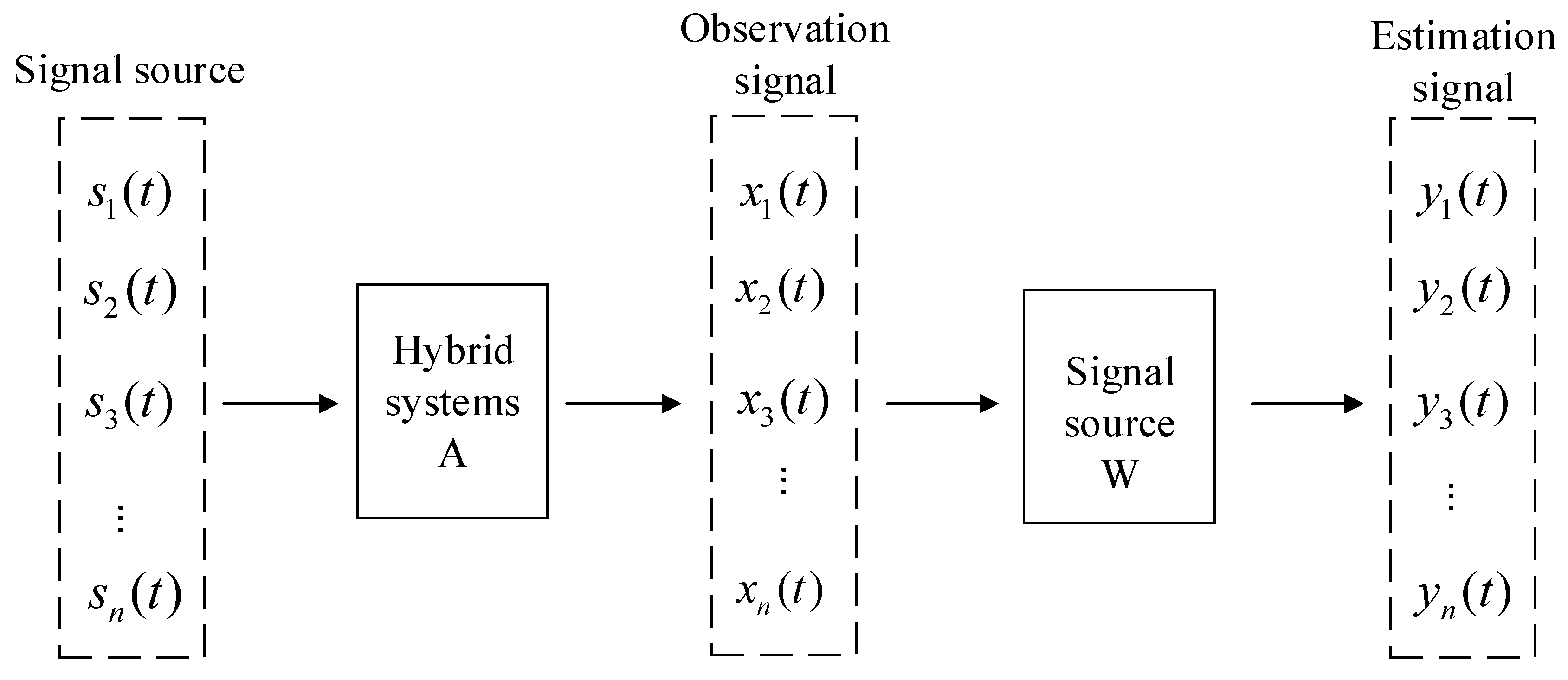
The method of fast independent component analysis (FICA) has the characteristics of fast convergence and good stability. It can weaken all kinds of interference information while protecting the useful signal. It has a wide application prospect in signal processing field. The FICA method is proposed for the original data to minimize the impact of the extreme conditions on the shock of the original sequence.

(c)

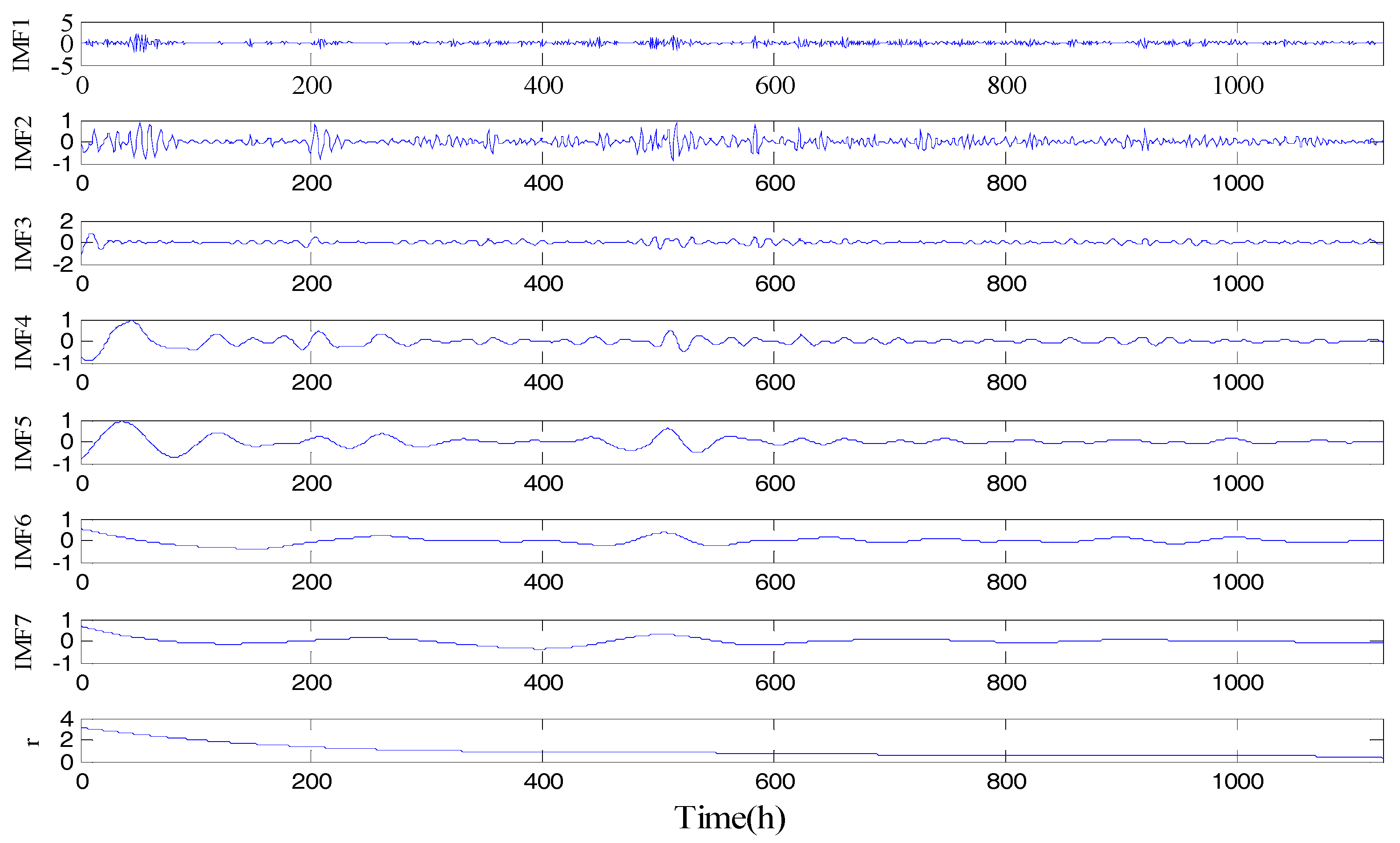
Ensemble empirical mode decomposition (EEMD) is a noise-aided data analysis method. This method avoids the difficulty of selecting wavelet bases in wavelet transform. Besides, it inherits the advantages of the empirical mode decomposition (EMD) method and also effectively solves the modal aliasing problem existing in the EMD process. As the thickness of ice cover is greatly affected by climatic factors, the regularity of the original data is not strong, and the sequence has non-stationary characteristics. To better reflect the internal structure of the original sequence, the data after denoising are decomposed by ensembling empirical mode decomposition (EEMD) into a high frequency and low frequency component.

(d)

The SVM is based on the principle of structural risk minimization. It can find the best compromise between the complexity and learning ability of the prediction model according to the information of the icing thickness sequence sample to obtain the best generalization ability. EEMD decomposes raw data into high-frequency and low-frequency component sequences with different complexity. In this paper, the optimal model parameters and kernel functions are selected according to the characteristics and complexity of each component, the SVM prediction model suitable for itself are established to improve the accuracy of single prediction model. The support vector machine model used in this paper is called the adaptive support vector machine model (ASVM).

(e)

A new hybrid algorithm, which is named of GATS, is presented by combining the genetic algorithm and tabu search. The hybrid algorithm effectively combines the parallel search capability of the genetic algorithm (GA) and the local search capability of the TS algorithm. The combined method can enhance the global search ability and improve the search speed.

(f)

The empirical results validate that the proposed model is suitable for ice cover prediction. The model can obtain higher accuracy and satisfactory results. The establishment of the model has important practical significance for the power grid enterprise to effectively confront ice disasters and ensure the safe and reliable operation of the power network [27].

2. Two-Stage Data Pre-Processing Method

2.1. Data De-Noising Processing by Fast Independent Component Analysis (FICA)

Independent component analysis (ICA) is a signal processing method developed in the 1990s. Initially, it was developed for the solution of blind signal separation. Recently, ICA has become a powerful tool for signal processing and data analysis [28,29].

ICA is essentially an optimization algorithm, namely, how to make the separating independent component close to each source signal. The standard ICA problem can be defined as:

Assuming that $x(t)={[x_1(t),x_2(t),\cdots ,x_m(t)]}^T$ is an M dimensional observation signal vector. It is linearly mixed with $N$ unknown and independent source signals $s(t)={[s_1(t),s_2(t),\cdots ,s_n(t)]}^T$, where $t$ is a discrete time and its value is $0,1,2\dots$. According to [28], the formula can be expressed as:

$$x(t)=As(t)$$

(1)

where $A$ is an $m\times n$ dimensional matrix, called the mixed matrix.

The basic idea of ICA is descriped as follows and seen in Figure 2.

In Figure 2, $s(t)$ is the source signals, $A$ is unknown mixed matrix, $x(t)$ is observed signal, and $W$ is separation matrix. The observed signal $x(t)$ is obtained by mixing the source signal $s(t)$ with the matrix $A$. In the case of the unknown mixed matrix $A$ and the source signals $s(t)$, the separation matrix $W$ is determined according to only the observed data vector $x(t)$, so that the output signal $y(t)={[y_1(t),y_2(t),\cdots ,y_n(t)]}^T$ is the estimation of the source signal $s(t)$, and $W$ is an $n\times m$ dimensional matrix. According to [29], the formula can be expressed as:

$$y(t)=Wx(t)=WAs(t)$$

(2)

The core of the ICA algorithm is to update $W$ to bring the estimation closer to the source signal. FICA is commonly used for the task. The FICA algorithm is also known as the fixed-point algorithm, uses the Newton iteration method to batch a large number of sampling points of the observed signal. An independent component is separated from the observation signal, which makes the convergence more rapid and stead, and the efficiency of the calculation is improved [30].

2.2. Data Decomposition by Ensemble Empirical Mode Decomposition (EEMD)

Empirical mode decomposition (EMD) is an adaptive signal processing method proposed by Huang in 1998. The method is used for non-linear and non-steady sequences and is directly aimed at data without determining the decomposition basis. EMD is relatively simple and easy to implement. The main idea is to use the Hilbert-Huang transform (HHT) conversion method to transform the non-linear and non-steady time sequence data into a steady sub-time sequence. The method is characterized by the introduction of the concept of the intrinsic mode functions (IMFs). The fluctuation or trend of different scales in the signal is decomposed into a series of data sequence with different feature scales, and each sequence is called an intrinsic mode function. IMF can be linear or non-linear, and each component has practical physical meaning [30]. However, they all have the same number of extreme points and zero crossing points, and there is only one extreme point between two adjacent zero crossing points. Additionally, any two IMF components are independent of each other.

Each IMF is superimposed, and residual component $r_n$ is the source signal. Compared to the method of frequency domain and time domain analysis, EMD is more suitable for the analysis of non-linear and non-steady signals [31].

For the traditional wavelet decomposition algorithm, empirical mode decomposition reduces the influence of human factors on the decomposition results, and has a certain advanced nature. However, in some cases, the algorithm shows the mode mixing phenomenon [32]. Ensemble empirical mode decomposition (EEMD) is a noise-assisted data analysis method aimed at eliminating the disadvantage of the mode mixing of EMD. EEMD includes the white Gaussian noise signals, which are continuous on different time scales, and can eliminate the noise effect by calculating the average of multiple noise processing results. The method solves the EMD mode mixed stack effectively. The basic principle of the EEMD method is as follows:

With the original signal $x(t)$, the EMD algorithm will decompose $x(t)$ into a set of IMF components $c_i$ and residual $r$, which is [32]:

$$x(t)={\displaystyle \sum _{i=1}^n{c}_i+r}$$

(3)

EEMD methods add Gaussian white noise to the original signal, using the uniform distribution characteristics of the Gaussian white noise frequency to make the signal in different time scales continuous to eliminate the frequency aliasing phenomenon. Gaussian white noise is subject to the normal distribution of $(0,{(\alpha \epsilon )}^2)$, where $\epsilon$ is the standard deviation of the signal and $\alpha$ is the strength parameter of the noise. The specific steps are as follows.

Gaussian white noise $n_i(t)$ with zero mean and constant standard deviation is added to the original signal $x(t)$. According to [33], the formula can be expressed as:

$$x_i(t)=x(t)+k\times n_i(t)$$

(4)

$n_i(t)$ is the noise added for the $ith$ time, and $x_i(t)$ is the signal after adding the noise the $ith$ time. $k$ is proportionality coefficient. It is generally believed that the standard deviation of the white noise added is 0.2 times of the standard deviation of the signal [34].

The following formula is obtained after decomposing noise signals [33]:

$$x_i(t)={\displaystyle \sum _{j=1}^n{c}_{ij}+r_i}$$

(5)

$c_{ij}$ is the $jth$ IMF component after EMD decomposition for the $ith$, and $r_i$ is the remainder after EMD decomposition for the $ith$.

Repeat the above steps for the $Nth$ EMD decomposition, calculate the IMF component and the remainder, and obtain the final IMF component $c_j$ and the residual. The formula can be expressed as [34]:

$$c_j={\displaystyle \sum _{i=1}^N\raisebox{1ex}{$c_{ij}$}\!\left/ \!\raisebox{-1ex}{$N$}\right.}$$

(6)

$$r={\displaystyle \sum _{i=1}^N\raisebox{1ex}{$r_i$}\!\left/ \!\raisebox{-1ex}{$N$}\right.}$$

(7)

The final result of the EEMD decomposition is [34]:

$$x(t)={\displaystyle \sum _{j=1}^n{c}_j+r}$$

(8)

2.3. Ensemble Empirical Mode Decomposition Based on Independent Component Analysis

The formation of ice cover is affected by climatic factors, such as wind direction, wind speed, temperature, humidity, etc. Therefore, collected ice thickness data is non-linear and non-steady, which will be the main factor affecting forecasting results. The effective denoising and decomposition of the ice thickness samples can reduce the non-stationarity of the signals. Independent component analysis belongs to the neural network category. The feature extraction method is not affected by strong background noise or strong interference signals. Fast independent component analysis (FICA) is applied to the signal decomposition to weaken the noise to signal interference, thereby the accuracy of signal decomposition and decomposition efficiency is improved. Ensemble empirical mode decomposition (EEMD) has a great improvement on the traditional empirical mode decomposition method [34]. It effectively solves the problem of mode superposition in traditional empirical mode, which makes the real signal get the maximum reservation. Combining the advantages of the two methods, the paper presents a new feature extraction method based on fast independent component analysis and empirical mode decomposition (FICA-EEMD). Firstly, the signals are separated into statistical independent components by FICA, and then the autocorrelation components of these statistical independent components are analyzed to eliminate the influence of environmental noise [35]. Next, the statistical independent components after denoised are decomposed by EEMD. The same frequency eigenmode function of each statistical independent component is cumulative reconstruction. Finally, extract the intrinsic mode function of ice thickness and constitute a new set of IMFs for the following predictions.

3. Improved Support Vector Machine Prediction Model

3.1. Adaptive Support Vector Machine (ASVM)

The basic idea of SVM is to use the non-linear mapping algorithm to convert the linear undecomposed samples in the low-dimensional space into the high-dimensional feature space, and then it can be divided into linear samples and analyzed by a linear method. SVM regression is used to build a non-linear mapping. The data will be mapped into a high dimensional feature space and a linear regression will be used for analysis [22,23,24]. Traditional modeling process for support vector machine is seen in [22,23,24].

An adaptive support vector machine (ASVM) model is proposed in this paper to improve the accuracy of the support vector machine prediction. The selection of the kernel function has a great impact on the veracity of prediction results of the model. By analyzing the complexity of the sample sequence, the kernel functions and parameters of different components are selected to improve the authenticity of the model. The SVM prediction model is established to obtain the final predictive value through component superposition.

3.2. Hybrid Optimization Algorithm of Genetic Algorithm and Tube Search

Genetic algorithm (GA) sets all individuals in the group as objects, and completes the adaptive search of the optimal solution of the problem through biological genetic and evolutionary selection, crossover and mutation mechanism simulation, complete the problem of the optimal solution of the adaptive search. It has the ability of parallel search, and can search for the optimal solution to solve the problem of multi-point departure from a solution space, which can preserve the historical information to a certain extent. It is applicable for the global optimization problem of large-scale arbitrary objective functions. However, GA also has shortcomings of poor local search ability and precocious termination phenomenon. If the algorithm has a small mutation probability, the introduction of new chromosomes is rare. On the contrary, the traditional mutation operator will lead to greater algorithmic randomness and make the search process too blind.

Similarly, due to its flexible memory function and contempt rules, the tube search (TS) algorithm can accept inferior solutions and a strong climbing capabilities in the process of searching. It can jump out of a local optimal solution to search the solution space in other fields, which increase the possibility of obtaining a better global optimal solution. However, the TS algorithm has over-reliance on the initial solution. The convergence rate of the algorithm will be affected by the poor initial solution, and the probability of obtaining the global optimal solution can be reduced due to move from one solution to another during the iterative search.

To improve the computing efficiency, the two algorithms are combined. First, the genetic algorithm is used for global search, which results in individual distribution in the solution space in most regions. Then, the TS search is performed for each individual to improve the quality of the group. The hybrid algorithm effectively combines the parallel search capability of the GA and the local search capability of the TS algorithm. Through the combination of the optimization algorithm, horizontal and vertical can combine to achieve global search. The specific calculation process is shown in Section 3.3. The basic theories and rules of the TS algorithm are found in [36], and the specific GA optimization process is described in [37,38]. We will not repeat those narrations in this paper.

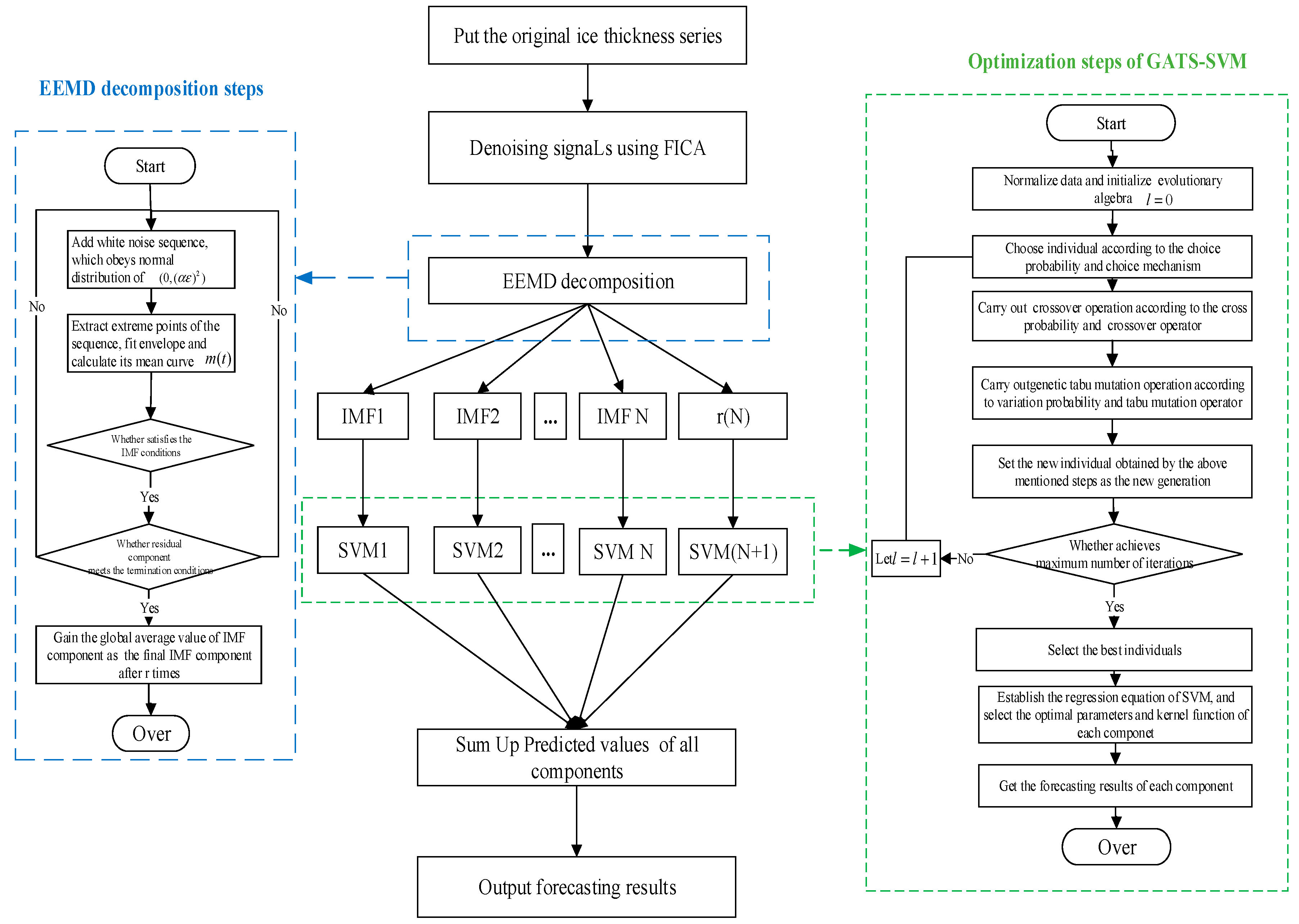
3.3. Modeling Process of the Adaptive Support Vector Machine Model Optimized by Genetic Tabu Search (GATS-ASVM)

Combining the characteristics of different intelligent algorithms, this paper optimizes the parameters of SVM based on the advantages of GA and tabu search (TS). Due to many uncertain natural climatic factors, the data of ice sheet thickness has great volatility and instability. Before forecasting, the original signal was decomposed by ensemble empirical mode decomposition, and the IMF components from high frequency to low frequency are obtained. According to the complexity of each component, different kernel functions of the support vector machine are selected for prediction. To improve the accuracy of the empirical mode decomposition, fast independent component analysis is adopted to perform the data preprocessing. As shown in Figure 2, the concrete forecasting steps include:

Step 1: Data preprocessing by FICA. Collect the real-time ice sheet sequences and use the FICA method based on the negative entropy to denoise the original signals. For $y(t)=Wx(t)$, $x$ is the original signal collected, and $W$ is the solution mixing matrix, which can separate the independent components $y$ in turn. For the multi-independent component decomposed, the useful signal and the noise signal are identified according to the prior knowledge of the signal time and frequency domain. Set the noise signal channels in the independent component to zero and reverse the original signal by the equation of $\widehat{x}(t)=W^{-1}y(t)$, where $\widehat{x}(t)$ is the signal after denoising.

Step 2: Data decomposition by EEMD. Use the EEMD to decompose the ice cover sequence $\widehat{x}(t)$ and obtain the IMF components $c_i(t)$ and the remainder $r_n$. Add the white noise sequence, which obeys normal distribution of $(0,{(\alpha \epsilon )}^2)$. Extract extreme points of the sequence, fit envelope and calculate its mean curve $m(t)$. After $x(t)$ minus $m(t)$, get a new signal $h(t)$. Then take the next step until $h(t)$ satisfies the IMF condition after screening $k$ times. The IMF component $h(t)$ is separated from the original signal, and the residual component $r(t)$($r(t)=x(t)-h(t)$) is obtained. The residual component $r(t)$ is used as the new raw data. Repeat the above steps and get the rest of the IMF component and 1 residual component.

Step 3: Normalization and initialization. Normalize the component data and initialize the evolutionary algebra $l=0$.

Step 4: Genetic tabu operation. Select the individuals based on the selection probability and selection mechanism. Cross-operation based on cross-probability and crossover operator. Perform the genetic tabu mutation operation according to the variation probability and tabu mutation operator.

Step 5: Convergence condition. The new individuals obtained by Step 4 are set to a new generation, the convergence conditions are determined: if the evolution algebra is less than the maximum number of iterations, then let $l=l+1$ and go back to Step 4; otherwise, terminate the network training, select the optimal individual, and continue to Step 6.

Step 6: Component prediction. Contract the SVM regression model for the IMF components $c_i(t)$ and $r_n$, select the best parameters and kernel functions, input the forecasting samples and the predicted values of each sequence are obtained.

Step 7: Final prediction. Superimpose each component forecast value to obtain the prediction value of the ice thickness.

In Figure 3, the graphics in the middle show the overall flow, the graph on the left shows the flow of ensemble empirical mode decomposition (EEMD) and the graph on the right shows optimization of support vector machines based on Genetic Tabu Search.

4. Case Study and Results Analysis

In this paper, a 220 kV DC transmission line in Hunan Province is used to verify the proposed model. The transmission line is an important transmission channel in Hunan with a total length of more than 80 km. Line monitoring data include leakage currents, ambient temperature, humidity, wind direction, rainfall and wind speed. Due to the influence of many factors, the time series of ice thickness of transmission line icing is disordered. According to the historical data, the prediction accuracy of the original data is determined, and other forecasting techniques are introduced for comparison.

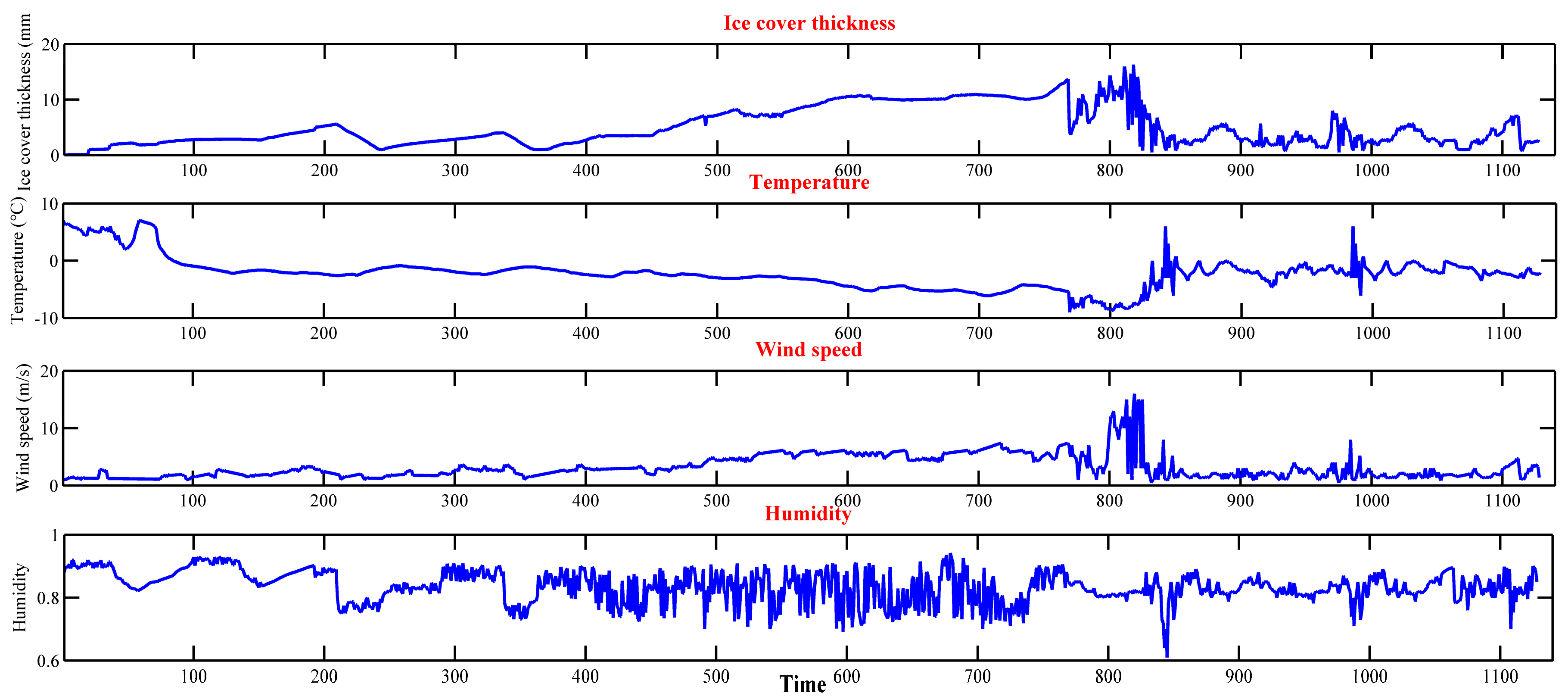
4.1. Data Preparation

Among the numerous factors influencing the power grid icing and meteorological factors is the most important factor, such as temperature, humidity, wind speed, wind direction and other external climate. A lot of scholars have studied the impact factors preliminary. Reference [39] summarizes the three necessary conditions for the formation of icing by reviewing the results of research of predecessors: Air relative humidity must be above 85%; wind speed should be greater than 1 m/s; the temperature has to reach 0 °C and below.

Analysis of the historical data shows that the most severe seasonal ice cover occurs in December, January, February, and March. On this basis, the main factors considered here are the temperature, relative humidity, and wind speed. Consequently, we choose the typical data for analysis. Per hour icing thickness and meteorological factors from 1 February 2014 to 19 March 2014 for the 220 kV transmission line are selected for the sample data. The raw data trend chart of ice cover thickness, temperature, relative humidity and wind speed are shown in Figure 4.

It can be seen from Figure 4 that the regularity of the ice cover thickness and the influencing factors are weak. There are more noises in the primitive sequence and the trend of the overall data is not strong. In general, the relative humidity fluctuates at 80%, the wind speed is greater than 0, while the temperature is lower than 0 degrees. On this basis, with the decrease of temperature, the increase of wind speed and relative humidity, the ice cover thickness shows an increasing trend. There is a strong correlation between the ice cover thickness and the selected three factors.

The figure above shows that the original sequence of ice thickness is out of order and has some fluctuations. The reprocessing of the original data is needed. Thus, before training samples, we must screen the raw data, adjust the missing data, and remove obvious errors. Finally, we retain 1128 sample points, of which the first 1000 sample points are selected as the training set and the remaining 128 sample points are used as the testing set to prove the validity of the model.

The forecasting model is solved through Matlab on a single core of a 32-bit Lenovo workstation running Windows 7 with 2 dual-core 2.60 GHz CPUs and 4.0 GB of RAM. We extract rules from the past information to forecast the ice cover thickness.

Due to the length limitations of the manuscript, the denoising and decomposition process of the influencing factors in Section 4.2 and Section 4.3 are not shown below. We just take ice cover thickness data as an example to show.

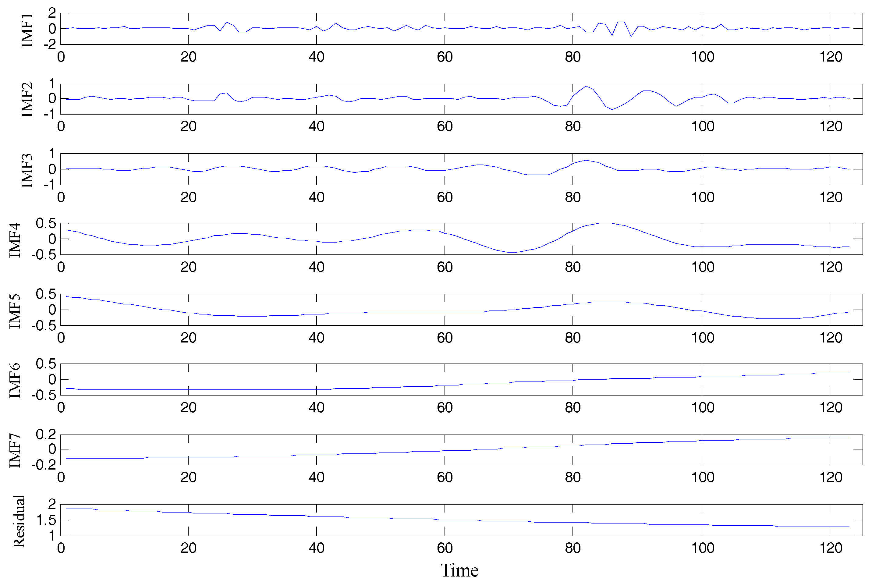
4.2. Data Preprocessing and Decomposition

Because the original data have large noise due to the abnormal points, the fast independent component analysis method is used to process with the original data to improve the model’s recognition before the decomposition of the EEMD model. Ice thickness data after denoising are decomposed into different sub-time series by the EEMD model, and the IMF component of a series of different scales is generated to achieve the stability sequences of the ice cover.

The EEMD method needs to determine the appropriate value of the strength parameters of noise $\alpha$ and decomposition number $n$. Reference [40] proved that we can gain greater results when $n=100$ and the $\alpha$ values range from 0.1 to 0.3. Thus, this paper selects $n=100$ and $\alpha =0.2$. EEMD decomposition of the time series of ice cover thickness is obtained by seven intrinsic mode components (from IMF1 to MF7) and a residual sequence. The results are shown in Figure 5. The EEMD decomposition process selects the intrinsic volatility components in the original sequence from high frequency to low frequency. The high-frequency components of high-frequency fluctuations are frequent and chaotic. In some places, the amplitude changes dramatically. The low-frequency components of the periodic law are relatively clear and have strong fluctuation.

4.3. Single Prediction

4.3.1. Selection of the Kernel Function

According to the characteristics of each component, the optimal model parameters and kernel functions are selected to establish the SVM model optimized by the genetic tabu search. The selection of the kernel function and its parameters are chosen to improve the accuracy of the sub-models by analyzing the complexity of the sample sequence, as seen in

Table 2. Complexity analysis of each component.

Mode	PE Values	Complexity
IMF1	0.99	High level
IMF2	0.782	High level
IMF3	0.573	High level
IMF4	0.441	Low level
IMF5	0.348	Low level
IMF6	0.254	Low level
IMF7	0.219	Low level
Residual	0.155	Low level

.

To capture the complexity features, the Permutation Entropy (PE) measurement is proposed [41]. It is a method to measure the complexity of time series. The value of permutation entropy represents the stochastic degree of time series. Generally speaking, the smaller the value, the more regular the time series. Otherwise, the time series is of more randomness. From IMF1 to the residue, the PE values gradually decrease from 1.0 to 0.1. Assuming that the threshold is 0.5, the PE values of IMF1 to IMF3 are all above the threshold value, indicating that the three modes have comparatively high-level complexity. In contrast, IMF4 to IMF7 and the residue have relatively low-level complexity because their PE values are all below the threshold. The radial basis kernel function (RBF) with better generalization capability and better processing nonlinear sequence is used for the intrinsic mode components IMF1, IMF2, and IMF3, which have large fluctuation frequency and high complexity; The polynomial kernel function is selected for IMF4, IMF5, IMF6 and IMF7, which have medium- and low-frequency components with the stable change. The residual component is predicted by the linear kernel function [42].

4.3.2. Single Prediction Results

The combined intelligent optimization algorithm of GA and TS is adopted to optimize the parameters $g$ and $C$ to determine an optimal parameter to improve the prediction accuracy of the model. The root mean square error ($RMSE$), mean absolute error ($MAE$) and mean absolute percentage error ($MAPE$) are set for the prediction effect evaluation of each model. The predictive value and the actual value of the model are, respectively, ${\widehat{y}}_i$ and $y_i$.

The corresponding formulas are as follows:

$$MAPE=\frac{1}{n}{\displaystyle \sum _{i=1}^n\left|\frac{{\widehat{y}}_i-y_i}{y_i}\right|}$$

(9)

$$RMSE=\sqrt{\frac{1}{n}{\displaystyle \sum _{i=1}^n{({\widehat{y}}_i-y_i)}^2}}$$

(10)

$$MAE=\frac{1}{n}{\displaystyle \sum _{i=1}^n\left|{\widehat{y}}_i-y_i\right|}$$

(11)

where $n$ represents the sample number.

Set the corresponding components of temperature, humidity and wind speed as input factors, corresponding components of ice thickness sequence as output factors, and put them into the SVM model, we can get the prediction results of each sub-sequence for the testing data as shown in Figure 6. The results of estimated errors in the predictions are given in Figure 7.

The instantaneous frequency of each IMF component has significant importance at any point. Different IMFs have different meanings, for instance, the low frequency band $IM{F}_n$ represents the trends of the data, whereas the highest frequency band IMF1 mainly contains noises. Figure 8 shows that the prediction error of $IM{F}_1$, which contains the signal of noises, is relatively large. The value of $MAPE$ is close to 200%, and the value of $RMSE$ and $MAE$ is much higher than those of other components. Thus, to improve the overall prediction accuracy and to retain the most important information, we remove the interference term IMF1 to achieve the purpose of the second-time denoising. The prediction results from $IM{F}_2$ to $IM{F}_7$ and the residual can be added to form the final prediction results.

4.4. Overall Forecasting Results and Error Analysis

Based on the above analysis, the predicted values of the components are superimposed to obtain the predicted values of the thickness of ice cover. The average percentage error $MAPE$ of the forecast value and the actual value are taken as the objective function to search the minimum value of the objective function as the target. The global minimum corresponding to the best fitness function value is the kernel parameter $g$ and penalty factor $C$ of the SVM model when the iteration terminates. The optimized parameters are used in the SVM prediction model to predict the ice thickness.

To investigate the performance of the intelligent model, four algorithms (non-preprocessing adaptive support vector machine optimized by genetic algorithm and tabu search (GATS-ASVM), support vector machine optimized by genetic algorithm (GA-SVM), and standard support vector machine (SVM)) are established for comparison to evaluate the effect of the intelligent model in ice cover thickness prediction. The prediction results of the comparison algorithms are shown in Figure 8.

Figure 8, Figure 9 and Figure 10 show the results of the four prediction models for forecasting of the thickness of ice cover and the actual measurement of the ice cover thickness. In general, the overall forecasting trends of the four models are close to the real value. The GATS-ASVM algorithm is the closest to the real curve, whereas the standard SVM prediction curves have some deviation.

Various error metrics between the real and forecasting data have been defined to assess the forecasting performance. In our experiments, $MAPE$ and $RMSE$ are introduced to appraise and compare the different simulation results.

Table 3. Error comparison of different algorithms.

Algorithm	MAPE (%)	RMSE (mm)
GATS-ASVM	5.22	1.81
Non-GATS-SVM	6.12	2.5
GA-SVM	6.47	3.51
SVM	7.78	4.68

and Figure 11 show the error distribution of the different models.

From Table 3 and Figure 8, Figure 9, Figure 10 and Figure 11, the following conclusions can be drawn:

(1)

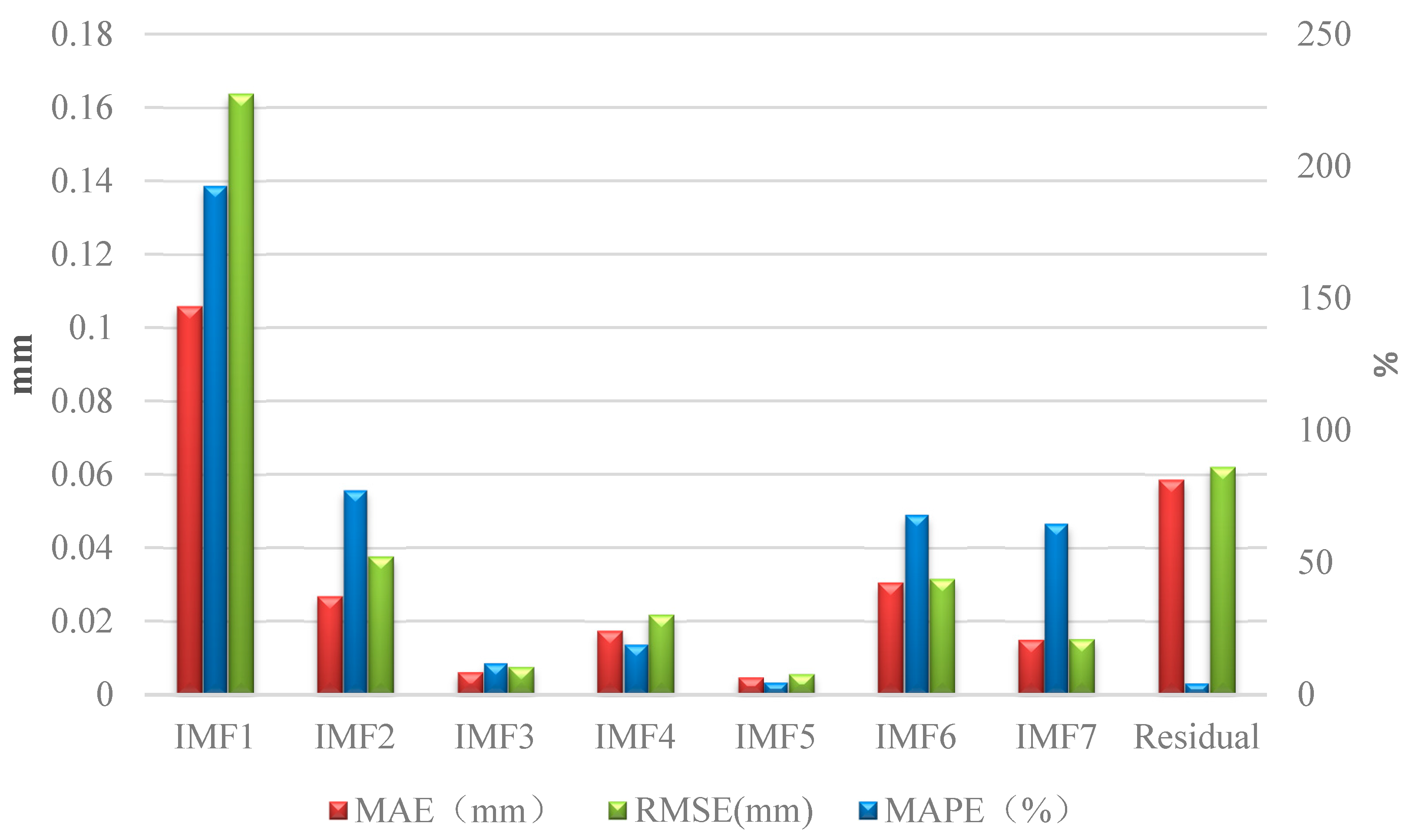
The results in Figure 8 and Figure 9 and Table 3 indicate that the model proposed in this paper with the processed data has significant advantages compared to the model with untreated data. Both the error metrics of MAPE and RMSE of the GATS-ASVM with data processing are less than the GATS-ASVM with untreated data because the EEMD method can separate different periods of the fluctuation signal from the original data to make the sub sequence data relatively orderly for higher forecast accuracy. At the same time, FICA denoising is necessary to make the processed data smoother.

(2)

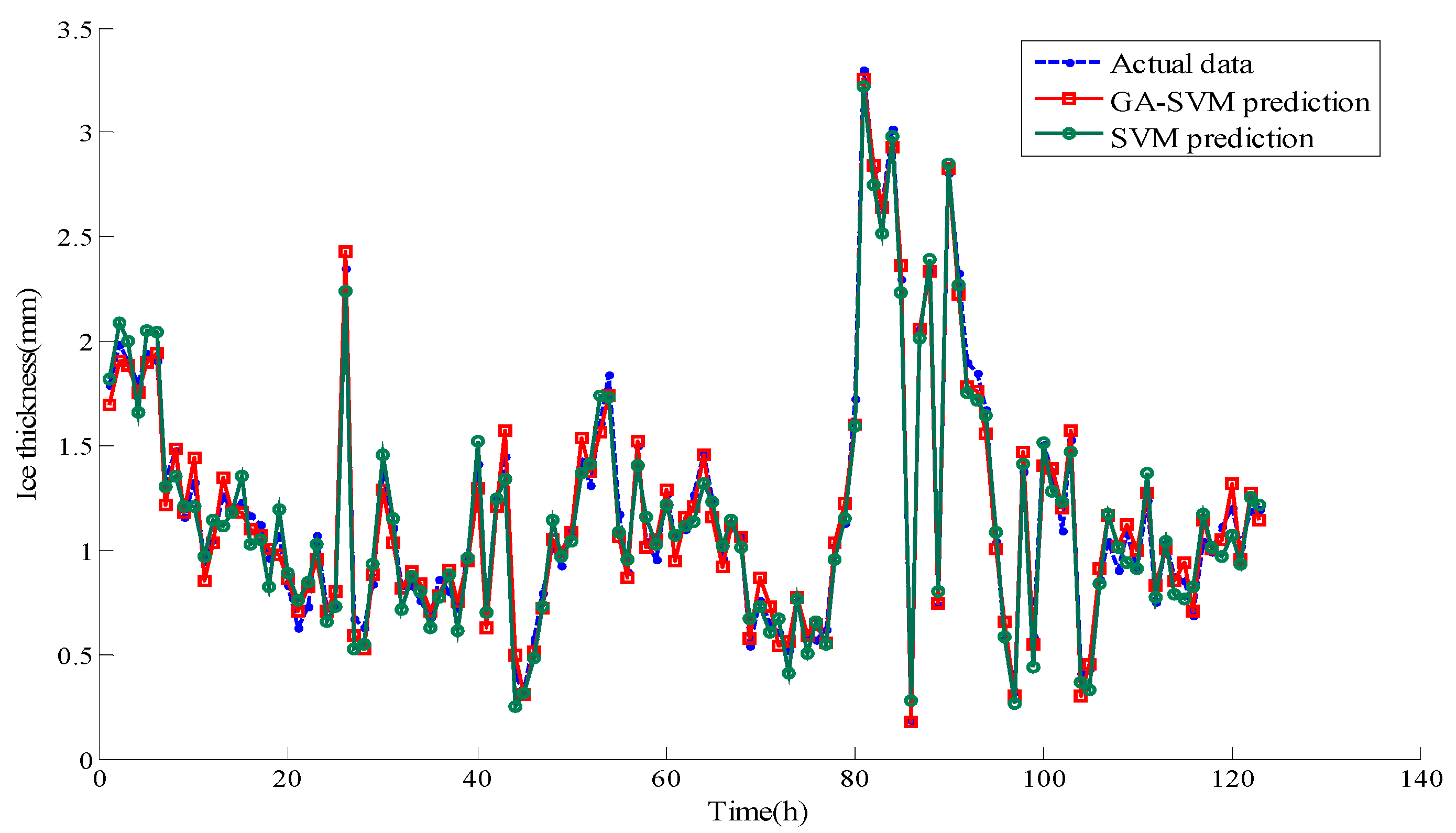
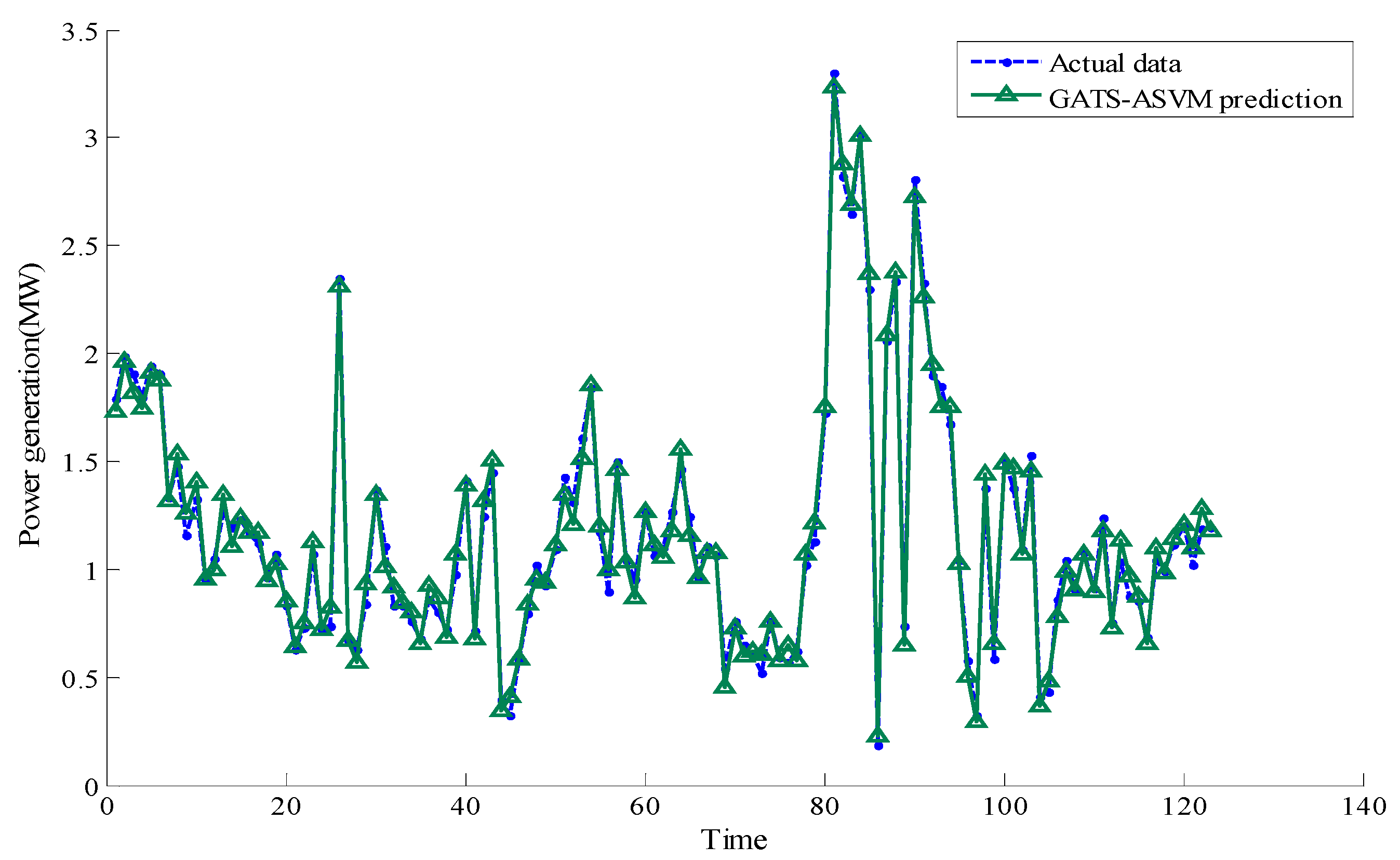
Comparing the GATS-ASVM model and GA-SVM model, the former has more advantages. The hybrid optimization algorithm makes up for the defects of the single algorithm, and the adaptive support vector machine takes into account the morphological characteristics of different sub-sequences and selects appropriate kernel functions, which improve the accuracy and the generalization ability of the model and result in better predictions.

(3)

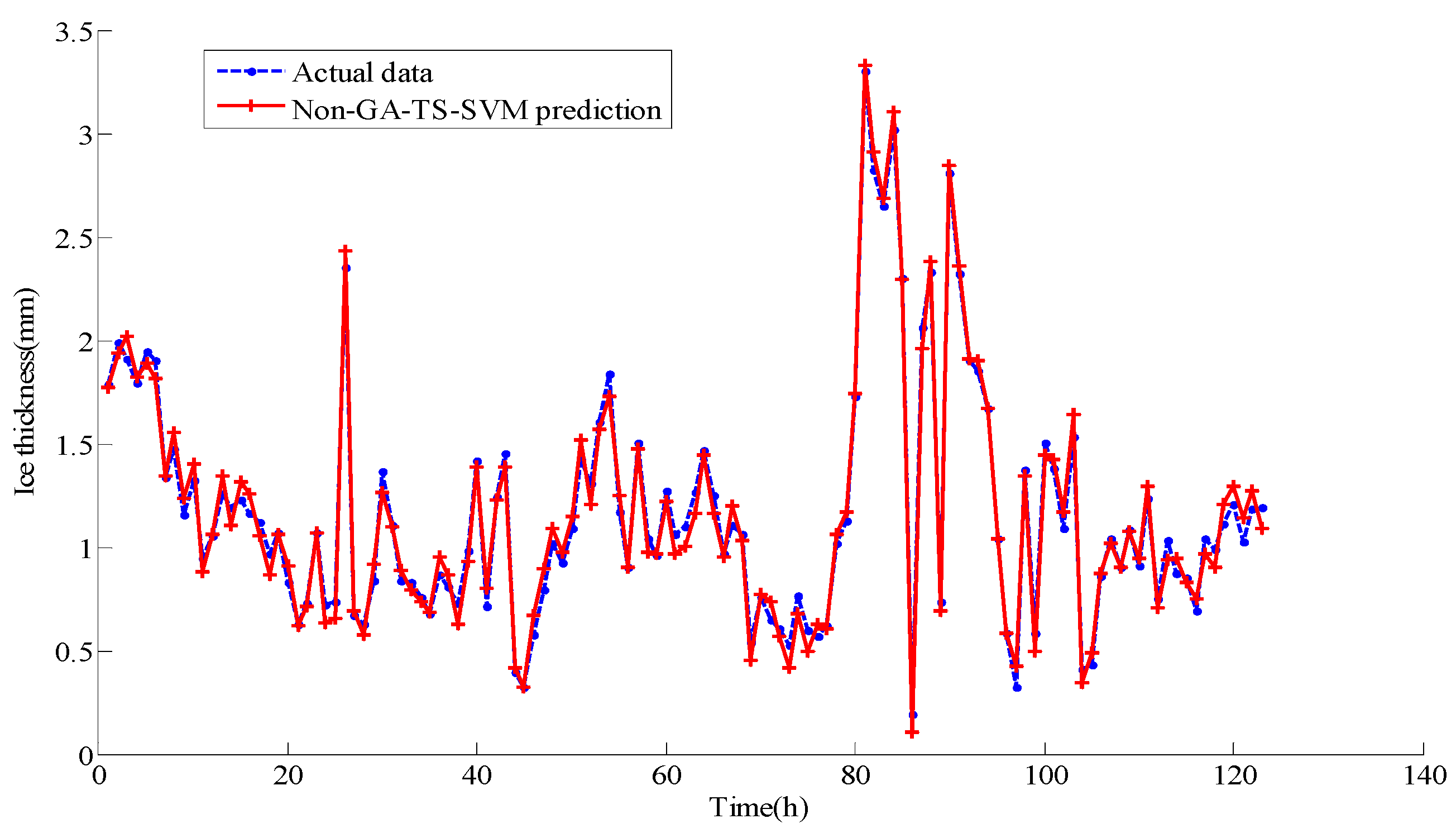
From Figure 8, Figure 9, Figure 10 and Figure 11 and Table 3, the forecasting precision of the combined model is higher than that of the single model. The combined forecasting model uses the complementary advantages of different algorithms to improve the accuracy of the algorithm. The prediction of the single model has large limitations.

(4)

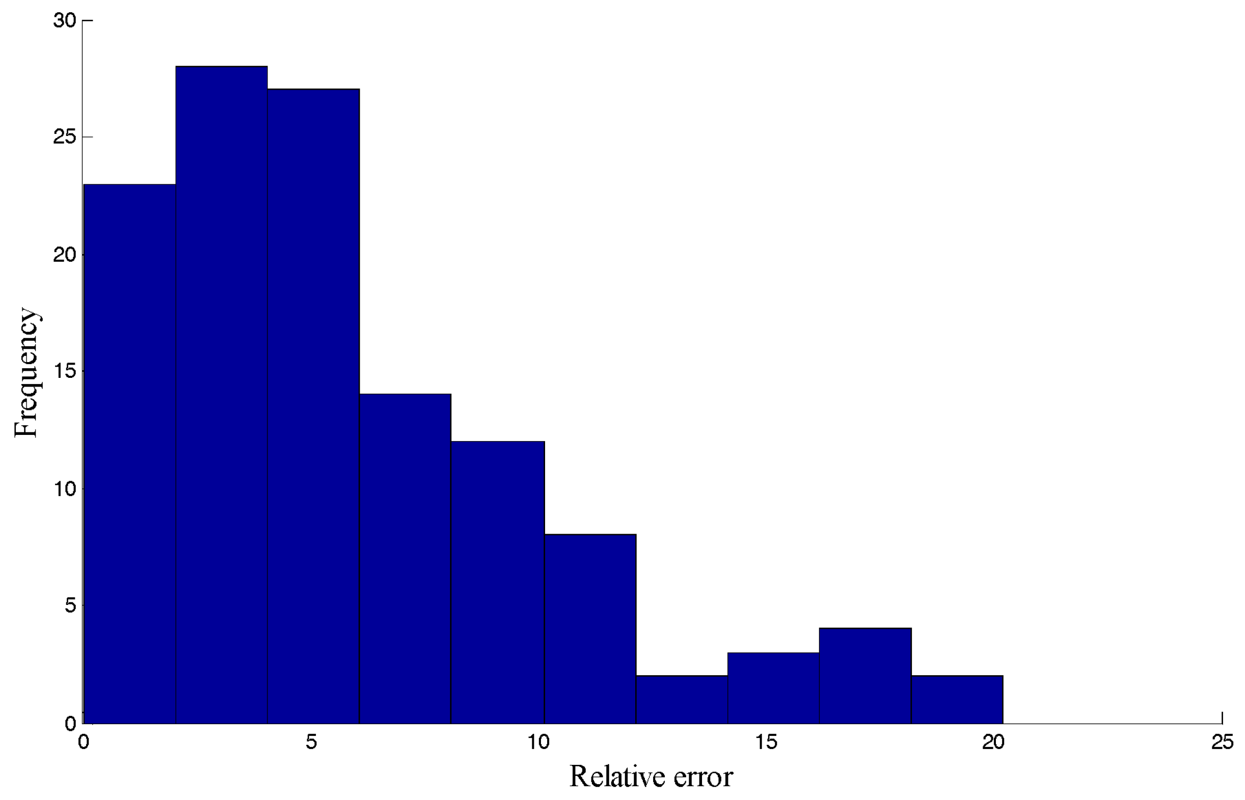
Figure 11 and Table 3 show less error in the proposed model. This model has a powerful function in the processing of non-stationary series. Figure 11 shows that the prediction error is controlled within 20%. Most of the errors are distributed between [0, 10%], and the error values greater than 10% are less common. The algorithm has a stable forecasting effect. The error evaluation results and the frequency histogram of the error distribution show that the adaptive support vector machine optimized by genetic tabu search based on ensemble empirical mode decomposition has higher prediction accuracy than other algorithms. Compared with the other three methods, the proposed GATS-ASVM method has obvious advantages and can be used for the prediction of the thickness of ice on transmission lines.

5. Conclusions

In this paper, an intelligent model is proposed to predict the thickness of ice cover on a transmission line. The model is useful for the power grid enterprise to effectively control the ice cover. It has great significance for the safe operation of power networks. Through the analysis and summary, this paper reaches the following conclusions:

Firstly, the raw data are processed by fast independent component analysis to remove the abnormal data in the extreme cases and gets great denoising results. The ensemble empirical mode decomposition decomposes data after denoising into different time frequencies from high frequency to low frequency so that the complex signal is decomposed into a finite intrinsic mode function.

Secondly, SVM model optimized by the genetic tabu search algorithm is presented to forecast each sub-sequence function after decomposition. The final icing prediction results are obtained by summing up the total sub-sequence forecasting results. Empirical analysis proves that the model proposed in this paper has strong robustness and generalization ability and can effectively overcome the shortcomings of the premature convergence of the genetic algorithm and the initial value dependence of tabu search. The SVM model is more stable, and the prediction accuracy is improved after optimization of the combined method.

To further improve the accuracy of the prediction, for different sub-sequence functions, the appropriate kernel functions are adaptively selected according to the complexity of the sample sequence to make the model more reliable. After comprehensive analysis of the situation of the transmission line icing on the 220 kV DC transmission line in Hunan Province, a numerical example is given to calculate the cover thickness of the ice cover in this transmission line from 1 February 2014 to 19 March 2014. The simular results of several different combinational algorithms demonstrate that the GATS-ASVM model is ideal for short-term ice cover thickness forecasting for grid transmission lines because it achieved better prediction accuracy.

References

1. Li, X.J. Research on Icing Forecasting Model of Transmission Line Based on Data Mining. Master’s Thesis, Taiyuan University of Technology, Taiyuan, China, 2016. [Google Scholar]
2. Li, P.; Zhao, N.; Zhou, D.H.; Cao, M.; Li, J.J.; Shi, X.L. Multivariable Time Series Prediction for the Icing Process on Overhead Power Transmission Line. Sci. World J. 2014, 2014, 256815. [Google Scholar] [CrossRef] [PubMed]
3. Li, C.G.; Lv, Y.Z.; Cui, X. The problem of safe operation of power grid in China under conditions of ice and snow disasters. Power Syst. Technol. 2008, 32, 14–21. [Google Scholar]
4. Shi, L.L. Assessment of Forest Damage caused by Ice Storm based on MODIS Data—A Case Study of Jiangxi Province, China. Disaster Adv. 2013, 6, 67–72. [Google Scholar]
5. Chang, H. Prediction and Experimental Study on Ice Thickness of Overhead Transmission Line Based on Dynamic Tension and Angle. Master’s Thesis, Chongqing University, Chongqing, China, 2013. [Google Scholar]
6. Liu, H.Z. DC Transmission Line Icing and Control; China Electric Power Press: Beijing, China, 2012. [Google Scholar]
7. Tian, L. Study on Icing Regularity and Optimal Configuration of Ice Handling Equipment in Hunan UHV Transmission Line. Master’s Thesis, Changsha University of Science & Technology, Changsha, China, 2013. [Google Scholar]
8. Li, Z.H.; Bai, X.M.; Zhou, Z.G.; Hu, Z.J.; Xu, J.; Li, X.J. The research progress of the method for the icing prevention and control of the power grid. Power Syst. Technol. 2008, 32, 7–14. [Google Scholar]
9. Li, P.; Li, N.; Cao, M.M. Micro-meteorology Features Extraction and Status Assessment for Transmission Line Icing Based on Intelligent Algorithms. J. Inf. Comput. Sci. 2010, 7, 2043–2052. [Google Scholar]
10. Dai, D.; Huang, X.T. Prediction of transmission line icing based on support vector machine model. High Volt. Technol. 2013, 39, 2822–2828. [Google Scholar]
11. Jiang, X.L.; Han, X.B.; Hu, Y.Y.; Yang, Z.Y. The study of Dynamic Wet-Growth Icing model of insulator. Proc. CSEE 2017, 09, 1–8. [Google Scholar]
12. Xu, Q.S.; Lao, J.M.; Hou, W.; Wang, M.L. Real-time monitoring and calculation model of transmission lines unequal ice-coating. High Volt. Eng. 2009, 35, 2865–2869. [Google Scholar]
13. Liu, H.Y.; Zhou, D.; Fu, J.P.; Huang, S.Y. A simple model for predicting glaze loads on wires. Proc. CSEE 2001, 21, 44–48. [Google Scholar]
14. Huang, X.B.; Wang, Y.X.; Zhu, Y.C.; Zheng, X.X.; Li, H.B.; Wang, Y.G. Line icing prediction based on genetic algorithm and fuzzy logic fusion. High Volt. Eng. 2016, 42, 1228–1235. [Google Scholar]
15. Zheng, Z.H.; Liu, J.S. Prediction method of ice thickness on transmission lines based on the combination of GA and BP neural network. Power Syst. Clean Energy 2014, 30, 27–30. [Google Scholar]
16. Liu, R.; Wu, X.D.; Yan, E.M.; Lang, L. Prominent influence factor analysis and RBF ice cover prediction of transmission lines. Electr. Appl. 2013, 32, 72–75. [Google Scholar]
17. Liu, J.; Li, A.J.; Zhao, L.P. Prediction model based on fuzzy and T-S neural network for ice thickness. Hunan Electr. Power 2012, 32, 1–4. [Google Scholar]
18. Wu, Q.D.; Yan, B. Displacement Prediction of Tunnel Surrounding Rock: A Comparison of Support Vector Machine and Artificial Neural Network. Math. Probl. Eng. 2014, 2014, 351496. [Google Scholar] [CrossRef]
19. Ma, T.N.; Niu, D.X.; Fu, M. Icing Forecasting for Power Transmission Lines Based on a Wavelet Support Vector Machine Optimized by a Quantum Fireworks Algorithm. Appl. Sci. 2016, 6, 54. [Google Scholar] [CrossRef]
20. Yin, Z.R.; Su, X.L. Icing thickness forecasting of transmission line based on particle swarm algorithm to optimize SVM. J. Electr. Power 2014, 29, 6–9. [Google Scholar]
21. Zhang, C.; Wei, H.K.; Zhao, J.S.; Liu, T.H.; Zhu, T.T.; Zhang, K.J. Short-term wind speed forecasting using empirical mode decomposition and feature selection. Renew. Energy 2016, 96, 727–737. [Google Scholar] [CrossRef]
22. Wei, T.X.; Ma, G.W.; Huang, W.B. Prediction of runoff based on penalized weighted support vector machine regression model. J. Hydroelectr. Eng. 2012, 31, 35–38. [Google Scholar]
23. Liang, J.J.; Wu, D. Smooth Diagonal Weighted Newton Support Vector Machine. Math. Probl. Eng. 2013, 2013, 349120. [Google Scholar] [CrossRef]
24. Xu, X.M.; Niu, D.X.; Wang, P.; Lu, Y.; Xia, H.C. The weighted support vector machine based on hybrid swarm intelligence optimization for icing prediction of transmission line. Math. Probl. Eng. 2015, 2015, 798325. [Google Scholar] [CrossRef]
25. Khan, A.; Jaffar, M.A. Genetic algorithm and Self Organizing map based fuzzy hybrid intelligent method for color image segmentation. Appl. Soft Comput. 2015, 32, 300–310. [Google Scholar] [CrossRef]
26. Gharehbaghi, S.; Khatibinia, M. Optimal seismic design of reinforced concrete structures under time-history earthquake loads using an intelligent hybrid algorithm. Earthq. Eng. Eng. Vib. 2015, 14, 97–109. [Google Scholar] [CrossRef]
27. Ye, Q.; Wang, M.; Han, J.R. Integrated risk governance in the Yungui Plateau, China: The 2008 ice-snow storm disaster. J. Alp. Res. Revue Geogr. Alp. 2012, 100, 100–112. [Google Scholar] [CrossRef]
28. Sardouie, S.H.; Albera, L.; Shamsollahi, M.B.; Merlet, I. An Efficient Jacobi-Like Deflationary ICA Algorithm: Application to EEG Denoising. IEEE Signal Process. Lett. 2015, 22, 1198–1202. [Google Scholar] [CrossRef]
29. Yao, J.C.; Xiang, Y.; Qian, S.C.; Wang, S.; Wu, S.W. Noise source identification of diesel engine based on variational mode decomposition and robust independent component analysis. Appl. Acoust. 2017, 116, 184–194. [Google Scholar] [CrossRef]
30. Xu, W.L.; Sun, T.; Hu, T.; Hu, T.; Liu, M.H. Huanghua Pear Soluble Solids Contents Vis/NIR Spectroscopy by Analysis of Variables Optimization and FICA. Spectrosc. Spectr. Anal. 2014, 34, 3253–3256. [Google Scholar]
31. Imaouchen, Y.; Kedadouche, M.; Alkama, R.; Thomas, M. A Frequency-Weighted Energy Operator and complementary ensemble empirical mode decomposition for bearing fault detection. Mech. Syst. Signal Process. 2017, 82, 103–116. [Google Scholar] [CrossRef]
32. Zeng, P.; Liu, H.X.; Ning, X.B.; Zhuang, J.J.; Zhang, X.G. Study on the energy distribution of the empirical mode decomposition for ECG energy distribution. Acta Phys. Sin. 2015, 64, 1–8. [Google Scholar]
33. Wang, H.; Hu, Z.J.; Chen, Z.; Ji, M.L.; He, J.B.; Li, C. A Hybrid Model for Wind Power Forecasting Based on Ensemble Empirical Mode Decomposition and Wavelet Neural Networks. Trans. China Electrotech. Soc. 2013, 28, 137–144. [Google Scholar]
34. Fan, L.J. The WPD-EEMD Method and Its Applied Research in the EEG Signals Processing. Master’s Thesis, Taiyuan University of Technology, Taiyuan, China, 2010. [Google Scholar]
35. Chen, J. Study of Denoising Method Based on Wavelet Transform and Independent Component Analysis. Master’s Thesis, Fudan University, Shanghai, China, 2010. [Google Scholar]
36. Qiu, H.; Ming, W.; Zhang, Z.Z. A tabu search algorithm for the multi-period inspector scheduling problem. Comput. Oper. Res. 2015, 59, 78–93. [Google Scholar]
37. Bukharon, O.E.; Bogolyubov, D.P. Development of a decision support system based on neural networks and a genetic algorithm. Expert Syst. Appl. 2015, 42, 6177–6183. [Google Scholar] [CrossRef]
38. Gan, L.K.; Shek, J.K.H.; Mueller, M.A. Optimised operation of an off-grid hybrid wind-diesel-battery system using genetic algorithm. Energy Convers. Manag. 2016, 126, 446–462. [Google Scholar] [CrossRef]
39. Lu, J.Z.; Jiang, Z.L.; Lei, H.C. The Hunan power grid in 2008 ice disaster accident analysis of power systems. Autom. Electr. Power Syst. 2008, 32, 16–19. [Google Scholar]
40. Wu, Z.; Huang, N.E. Ensemble empirical mode decomposition: A noise-assisted data analysis method. Adv. Adapt. Data Anal. 2009, 1, 1–41. [Google Scholar] [CrossRef]
41. Yu, L.; Wang, Z.S.; Tang, L. A decomposition–ensemble model with data-characteristic-driven reconstruction for crude oil price forecasting. Appl. Energy 2015, 156, 251–267. [Google Scholar] [CrossRef]
42. Lin, Y.; Liu, P. Combined Model Based on EMD-SVM for Short-term Ice thickness Prediction. Proc. CSEE 2011, 31, 102–107. [Google Scholar]
Figure 1. Maximum ice cover thickness data of a transmission line in Hunan Province from 2000 to 2015.
Energies 10 01862 g001
Figure 2. Basic principle diagram of independent component analysis (ICA).
Energies 10 01862 g002
Figure 3. Model structure diagram for ice cover thickness forecasting.
Energies 10 01862 g003
Figure 4. Original data of ice cover thickness, temperature, wind speed and relative humidity from 1 February to 19 March 2014.
Energies 10 01862 g004
Figure 5. Fast Independent Component Analysis and Ensemble Empirical Mode Decomposition (FICA-EEMD) of the ice thickness.
Energies 10 01862 g005
Figure 6. Prediction results of each component for the testing data.
Energies 10 01862 g006
Figure 7. Prediction error of each component for the testing data.
Energies 10 01862 g007
Figure 8. Curves of the proposed model forecasting results and the actual ice thickness.
Energies 10 01862 g008
Figure 9. Curves of proposed model forecasting results without data processing. Note: “non- adaptive support vector machine optimized by genetic algorithm and tabu search (GATS-ASVM) prediction” means prediction results of the proposed method without data processing (including fast independent component analysis (FICA) and and ensemble empirical mode decomposition (EEDM)).
Energies 10 01862 g009
Figure 10. Curves of the comparison model forecasting results.
Energies 10 01862 g010
Figure 11. Frequency histogram of the error distribution for the GATS-ASVM algorithm.
Energies 10 01862 g011