Pre-Arcing Time Prediction in a Making Test for a 420 kV 63 kA High-Speed Earthing Switch

Abstract

A high-speed earthing switch (HSES) of a gas-insulated switchgear (GIS) performs a secondary role in protecting the power system in the event of an accident. After being interrupted by a circuit breaker (CB), the short-circuit current remaining in the network should be earthed by the HSES. However, as the contacts of the HSES may have been damaged by a pre-arc during the closing operation, the HSES may fail to ground the short-circuit current. To successfully ground the short-circuit current, the contacts of the HSES must be protected from damage by the pre-arc. Thus, minimizing the pre-arcing time is required to step up the making performance. This paper analyzes the making performance of the HSES by predicting the pre-arcing time within the short-circuit current making test. To estimate the pre-arcing time, we compared the results of analytical calculations based on streamer discharge theory and the numerical simulations of the electric field strength. By conducting a short-circuit current making test for a 420 kV 63 kA HSES in a high-power laboratory, the pre-arcing time calculation results were verified. A comparison of the results showed that the proposed prediction method was useful for verifying the performance of the HSES.

1. Introduction

A gas-insulated switchgear (GIS) is a protective device that prevents the spread of a fault current in the power systems to increase the reliability of a power system [1]. When a short-circuit current occurs, the circuit breaker (CB) of the GIS separates the other systems from the accident spot primarily. To clear the interrupting operation, the high-speed earthing switch (HSES) of the GIS should earth the short-circuit current remaining in the networks as a secondary protection operation [2]. However, as the contacts of the HSES may have been damaged by a prestrike arc during the closing operation, the HSES may fail to ground the short-circuit current [3,4]. The high temperature arc plasma within the HSES lasts for several milliseconds during the pre-arcing time. To successfully ground the short-circuit current, the contacts of the HSES must be protected from the high temperature arc plasma. Thus, minimization of the pre-arcing time is the most important factor for protecting the contacts. Much research has been conducted on minimizing arc duration to prevent contact erosion [5,6,7,8,9]. The previous approaches described in References [5,6,7,8,9] focused on the analysis of the arc-flash impact in consideration of the arc duration for HSES, CB, and vacuum circuit breaker (VCB). In particular, the efficiency of the minimization of arcing time was verified in Reference [6] to reduce incident energy and associated hazards in medium voltage systems. To minimize the pre-arcing time during the closing operation in a VCB, the authors in Reference [9] optimized the closing velocity, which can reduce percussion welding from the arc energy in a VCB. To reduce the pre-arcing time, increasing the mechanism speed is the most certain approach. Thus, a motor spring mechanism is generally adopted, as the operating system can enable fast movements using the charged spring energy. The researchers in References [10,11] showed that enough speed generated by the charged spring energy could allow the HSES to successfully earth the short-circuit current in the making test. However, it was impossible to increase the speed infinitely as the mechanism is overloaded. Therefore, this paper set a sufficient operating speed within the appropriate spring energy for the HSES mechanism.

On the other hand, much research has also been conducted in predicting breakdown phenomena by numerical simulation, experimental approaches, and statistical estimations [12,13,14,15]. However, less research exists for estimating the pre-arcing time from the perspective of dielectric breakdown phenomena in the making process of the HSES. This paper proposes a pre-arcing time prediction method in the HSES by comparing the analytical calculation results of the breakdown moment and the numerical simulations of the electric field strength. The pre-arc that occurs during a closing operation commences with the dielectric breakdown caused by the applied voltage stress. In other words, the pre-arc lasts from the commencement of dielectric breakdown until the moment the contacts touch each other. Therefore, it is very important to find the breakdown initiation moment for calculating the pre-arcing time of the HSES. The breakdown moment is calculated based on streamer discharge theory, as many researchers have analyzed the dielectric process in SF₆ insulation technology using the streamer discharge theory [16,17,18]. In particular, partial discharges and breakdown at protrusions in uniform electric fields in SF₆ have been discussed in both experimental and theoretical ways in Reference [16]. The steamer radius and length, which are important parameters for breakdown process, were experimentally investigated in Reference [17]. The formulation of the breakdown voltage was well organized and the condition to build a streamer in SF₆ was introduced in Reference [18]. Using the breakdown formulation in Reference [18], this paper suggests a process for predicting the pre-arcing time for the HSES making performance by comparing the results from the theoretical calculations and numerical simulations. Moreover, a development test was conducted to verify the making performance of the HSES by applying a 63 kA short-circuit current in a high-power laboratory.

The remainder of the paper is organized as follows. Section 2 explains the pre-arcing time calculation method, which considers the estimated breakdown electric field strength based on streamer discharge theory. Section 3 introduces the conditions of the making test for a 420 kV 63 kA HSES according to the international standard. Section 4 introduces the closing operation timing measurement data of the HSES motor spring mechanism. Using the finite element method, Section 5 conducts three-dimensional electric field simulations of the 420 kV 63 kA HSES making process to predict the pre-arcing time. Then, a comparative analysis between the simulation and experimental results is shown to verify the accuracy of the theoretical prediction using this calculation method. In addition, this paper inspects the state of the contacts after the laboratory tests to analyze the impact of arc energy. Finally, Section 6 contains the conclusions of this study.

2. Streamer Discharge Theory

The dielectric strength of SF₆ is relatively high when compared to that of other insulating gases, due to its electron affinity. The electron affinity of an atom or a molecule is defined as the amount of energy released when an electron is added to a neutral atom or a molecule in a gaseous state to form a negative ion. In general, halogen atoms release the highest amounts of energy (F = 3.40 eV, Cl = 3.61 eV, Br = 3.36 eV, I = 3.06 eV) to gain an electron, as they become more stable when a filled valence shell is obtained [19]. Therefore, the electron affinity of SF₆, which contains six fluorine atoms, is comparatively higher than that of common gases. Because of its high electron affinity, SF₆ has a high insulating performance as it combines with free electrons generated in the electric field. Nevertheless, when a high electric field is applied, the SF₆ molecules are ionized and produce many free electrons via a self-propagation process.

The discharge phenomenon in a gas begins when an electron avalanche is built up in a process where a number of free electrons are subjected to strong acceleration by an electric field. This ionization process occurs when the ionization coefficient α exceeds the electron attachment coefficient η. The ionization coefficient α indicates the degree to which gas molecules are ionized in the electric field, and the electron attachment coefficient η indicates the degree to which gas molecules recombine with free electrons. In accordance with the streamer discharge theory, such an electron avalanche grows to be a streamer via self-propagation through the stronger electric field formed by the space charge in a gaseous medium, as shown in Figure 1. As the electron velocity is faster than the positive-ion velocity, the cone-shaped space charge will extend over the entire discharge [20].

The average number of electrons in the avalanche at the moment when the number of electrons exceeds that of the positive ions is given by N_crit. After exceeding N_crit, the electron avalanche gradually progresses as a streamer. The authors in Reference [18] introduced the following relationship to calculate N_crit.

$$\ln N_{crit}={\displaystyle {\int }_0^{x_{crit}}\left(\alpha -\eta \right)}dx.$$

(1)

In Equation (1), x_crit is the critical distance where α = η. The author in Reference [21] suggested that the critical value N_crit reached the order of 10⁸ regardless of gas type or the field uniformity, and Reference [18] took N_crit as 10⁸. To calculate the effective ionization coefficient α′ = α − η, the linear relation between α′ and (E/P) is given as follows [18]:

$$\frac{{\alpha }^{\prime }}{P}=\frac{\alpha -\eta }{P}=K\left[\frac{E}{P}-{\left(\frac{E}{P}\right)}_{crit}\right]$$

(2)

where

$$K=27[{\mathrm{kV}}^{-1}],{\left(\frac{E}{P}\right)}_{crit}=89[\mathrm{kV}/(\mathrm{cm}\cdot \mathrm{atm})].$$

The critical value (E/P)_crit of SF₆ is 3.3 times that of air, which helps to maintain an improved dielectric performance. It is well known that the dielectric strength of air is 30–40% that of SF₆. By substituting Equation (2) into Equation (1), the breakdown electric field E_bd can be calculated from the following equation [18]:

$$\ln N_{crit}=K\left[{\displaystyle {\int }_0^{x_{crit}}E(x)}dx-{\left(\frac{E}{P}\right)}_{crit}\cdot P\cdot x_{crit}\right].$$

(3)

In a uniform electric field, E(x) and x_crit become constant so that the integral term can be worked out as $E_{bd}^{\max }$ × l where $E_{bd}^{\max }$ is the maximum breakdown electric field strength and l is the gap length. In the case of non-uniform electric fields, E(x) and x_crit are not constants; rather, they are functions defined as follows:

$$E(x)=\frac{E_{bd}^{\max }}{{(1+x/R)}^2}$$

(4)

and

$$x_{crit}=R\left(\sqrt{\frac{E_{bd}^{\max }}{{(E/P)}_{crit}\cdot P}}-1\right)$$

(5)

where

$$\frac{1}{R}=\frac{1}{2}(\frac{1}{R_1}+\frac{1}{R_2}).$$

(6)

In the above equation, R is the harmonic radius of positive and negative poles under the condition that x_crit is relatively small compared to R₁ and R₂. By substituting Equations (4) and (5) into Equation (3), the following can be obtained:

$$\frac{E_{bd}^{\max }}{P}={\left(\frac{E}{P}\right)}_{crit}\left(1+\frac{m}{\sqrt{PR}}\right)$$

(7)

where

$$m=\sqrt{\frac{4\ln N_{crit}}{K{\left(E/P\right)}_{crit}}}=0.175\left[c{m}^{1/2}\cdot at{m}^{1/2}\right].$$

(8)

Based on the relation: u = $E_{bd}^{av}/E_{bd}^{\max }$, where u is the field utilization factor, the average breakdown electric field strength can be derived as follows:

$$E_{bd}^{av}={\left(\frac{E}{P}\right)}_{crit}\cdot u\cdot P\cdot \left(1+\frac{m}{\sqrt{PR}}\right)$$

(9)

where

$$u=\frac{1}{0.6162\cdot {(l/R)}^{0.9716}+1.1377}.$$

(10)

Since the range of l/R given by the utilization factor in Reference [22] as 0.8 ≤ l/R ≤ 40 fit well for our HSES model, we used it in the following equation. This breakdown criterion can be improved when we consider the surrounding temperature condition [23].

3. Making Test Conditions

During the making test, the HSES goes through three intervals between contacts: a high-voltage interval, a pre-arcing interval, and a latching interval [10,11]. Among these three intervals, this paper focused on the pre-arcing interval, which gave the most severe conditions to the HSES. In References [10,11], these three intervals are defined as follows:

• The high-voltage interval is the time from the commencement of the test to the moment of breakdown (from commencement to t₀).
• The pre-arcing interval is the time from the moment of breakdown across the contact gap to the touching of the contacts (from t₀ to t₁).
• The latching interval is the time from the touching of the contacts to the moment when the contacts reach the fully closed (latched) position (from t₁ to t₂).

The three moments of t₀, t₁, and t₂ are shown in Figure 2. t₀ is the moment that the short-circuit current begins to flow, t₁ is the moment of contact touch, and t₂ is the moment that the closing operation finishes. For the short-circuit making test, the HSES should be subjected to symmetrical and asymmetrical test procedures in accordance with

Table 1. Procedures for the short-circuit current making test.

Procedures	Conditions	Outputs
Symmetrical	Making at the peak of the voltage wave with a tolerance of −30 electrical degrees to +15 electrical degrees	Symmetrical short-circuit current with the longest per-arcing time
Asymmetrical	Making at the zero of the voltage wave	Asymmetrical short-circuit current without pre-arcing

[24]. The symmetry of short-circuit making current is determined by the time of the making moment. If both contacts of the HSES make at the peak value of the rated voltage with a tolerance of −30 electrical degrees to +15 electrical degrees, the short-circuit making current flows symmetrically, leading to the longest pre-arcing time. Meanwhile, the asymmetrical current flows between contacts with no arc when they make at the voltage zero point. Therefore, the two moments of t₀ and t₁ are the same. Figure 2 presents two examples of making test waveforms that are (a) symmetrical and (b) asymmetrical short-circuit currents for the HSES. As shown in these waveforms, for the symmetrical case, the short-circuit current began near the voltage peak position, and the pre-arc exists until the contact touch point. For the asymmetrical case, the short-circuit current occurred at the voltage zero without generating a pre-arc.

In this paper, we introduce the experimental results of a 420 kV 63 kA HSES making test conducted in the high-power laboratory of the Korea Electro-Technology Research Institute (KERI) [25]. Given our test object was a single-phase enclosed switchgear model, the applied voltage was $U_r/\sqrt{3}$, where U_r is a rated voltage of 420 kV, with a peak value of approximately 343 kV [24].

4. Closing Operation Timing Measurement

Given that the HSES has to endure the pre-arc energy for a few milliseconds, the moving contact requires high-speed operation to maintain the current carrying performance by reducing the pre-arcing time. In general, when using spring energy, the HSES can operate faster than when relying solely on motor energy. We designed the mechanism to operate at 3.5 m/s in our HSES model. Although the faster speed of the mechanism maintained the shorter pre-arcing time, increasing the speed of the mechanism was bounded due to size and endurance limitations. Therefore, the proper design of the spring characteristics is extremely important for regulating the speed of the mechanism within an acceptable range.

Table 2. Tension spring characteristics for the 420 kV high-speed earthing switch mechanism.

Symbol	Meaning of Symbol	Value
d	10 mm	Wire diameter
D	Average diameter	47.5 mm
D2	Outer diameter	57.5 mm
Na	Number of active coils	17 turns
G	Shear modulus of elasticity	8000 N/mm2
L	Free length	275 mm
P1	Load for stretching 25 mm	203.22 N
P2	Load for stretching 65 mm	422.87 N
k	Spring constant	5.49 N/mm
τ1	Shear stress by P1	24.59 N/mm2
τ2	Shear stress by P2	51.15 N/mm2

presents the characteristics of the tension spring adopted in our mechanism.

To establish the tension force from which we intended to obtain an operation speed of 3.5 m/s, tension tests were conducted by stretching the spring length to 25 mm and 65 mm. The spring constant and shear stresses in Table 2 were calculated using Equation (11) [26].

$$k=\frac{G{d}^4}{8N_a{D}^3}, {\tau }_i=\frac{8D{P}_i}{n{d}^3}.$$

(11)

In the pre-arcing time prediction process, it was necessary to measure the closing time (the time interval from the closing coil current was activated from the instant when the arcing contacts touch each other) and the real travel distance data accurately in the closing operation timing measurement. By applying the tension spring (using the specifications in Table 2) to the HSES, several rounds of no-load closing operation tests were performed. During a laboratory test for the HSES, the closing time deviation that considered the solenoid, latch, and contact touch durations had to be kept uniform [2]. In general, the high-power laboratory suggested that the deviation of the closing time should be within ±1 ms. Thus, before the laboratory test, to check the deviation of the closing time, the closing operation timing measurements were carried out over 10 times. As a result, the average closing time was measured as 78.42 ms with a standard deviation of 0.49 ms and the average closing speed was calculated to be approximately 3.56 m/s, which met our intended operation speed. The travel distance data of the closing operation timing measurement is shown in Figure 3.

5. Simulation and Experimental Results

Before conducting the HSES making tests in a high-power laboratory, three-dimensional electrostatic simulations were conducted using the commercial software, COMSOL Multiphysics, to predict the pre-arcing time of the test model. For the reference breakdown electric field strength, a breakdown formula that considered the streamer discharge theory introduced in Section 2 was utilized.

5.1. Simulation Results

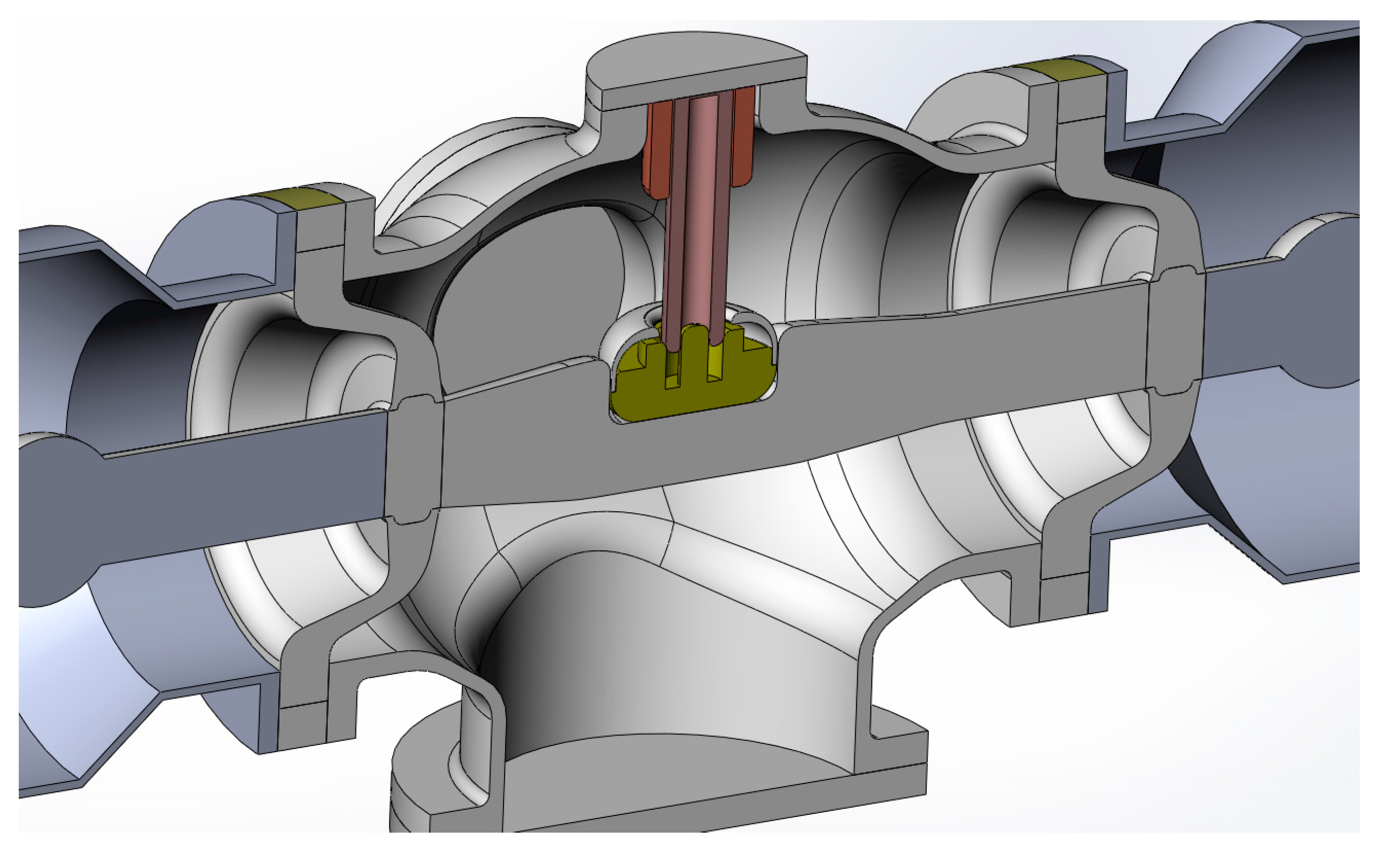
Using the same model as that of the laboratory test specimen, and adjusting the real travel distance data, the electric field strength between the fixed and moving contacts was calculated by traveling from the open position to the closed position. Figure 4 presents a simplified three-dimensional analysis model for the HSES.

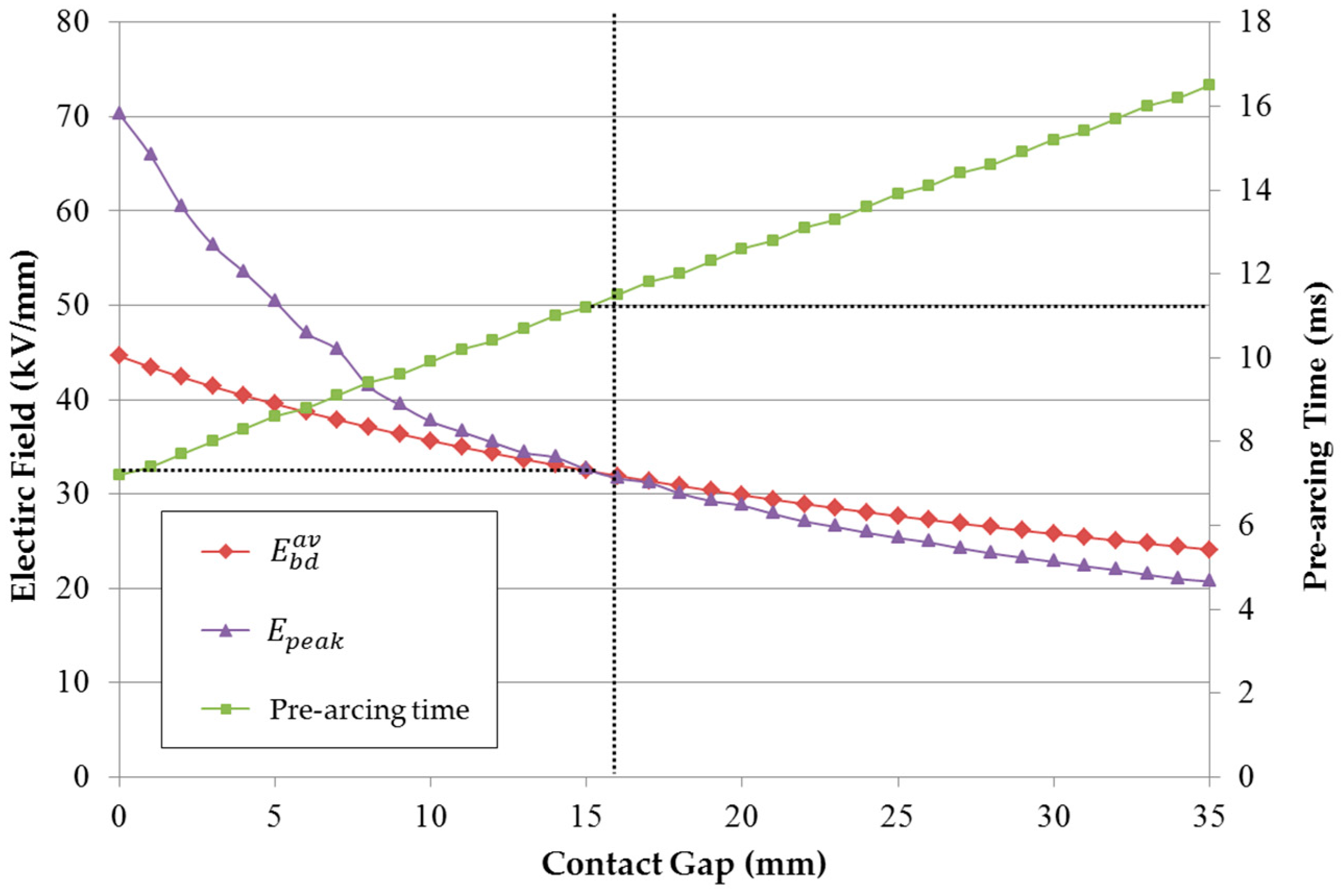
As mentioned in Section 3, the rated peak voltage of a single-phase making test for 420 kV was 343 kV; therefore, we used this voltage as a boundary condition in the electrostatic simulation. To calculate the average breakdown electric field in Equation (9), we set the absolute gas pressure of SF₆ as 0.55 MPa and the harmonic average radius of the contacts of our HSES model. The graph in Figure 5 shows the results of the comparison between the average breakdown electric field strength ($E_{bd}^{av}$) and the peak value of electric field distribution (E_peak) in the electrostatic numerical simulation.

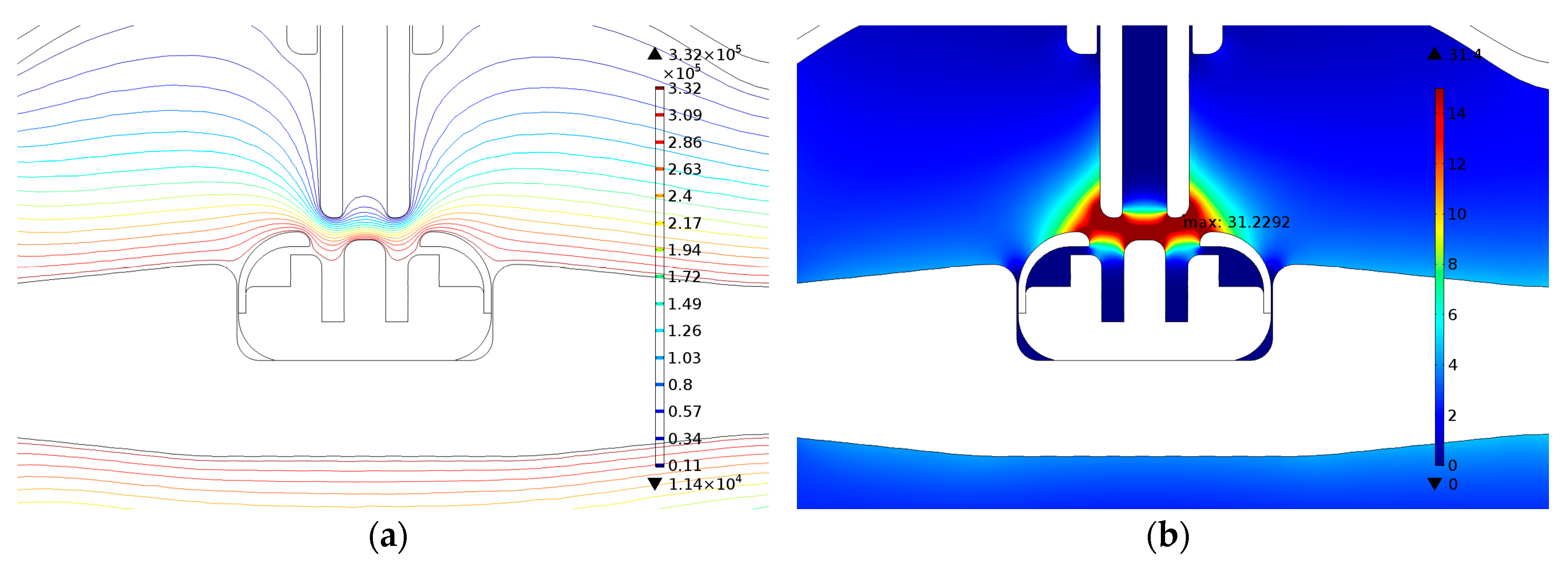
When the moving contact of HSES approached the fixed contact, the breakdown and simulated electric field strengths increased until the moment the contacts touched. However, the increase rate of the peak value of electric field strength in the simulation was faster than that of the average breakdown electric field; hence, a magnitude reversal point existed between the two lines at an approximately 15 mm contact gap. At this point, dielectric breakdown was initiated, inducing a pre-arc between the contacts. The pre-arc was maintained for 11.2 ms. The electric potential and field distribution results at this gap are shown in Figure 6.

Figure 7 shows the three-dimensional analysis results of the breakdown factor λ, which was defined as the ratio of the simulated and average breakdown electric field strengths ($E_{peak}/E_{bd}^{av}$) in this paper. After the breakdown moment, the maximum value of the simulated electric field increased above the breakdown reference; therefore, λ became greater than 1. As shown in Figure 7b, it was observed that the breakdown factor λ increased more rapidly when compared to the field utilization factor u, as the contact gap decreased to the moment when the arcing contacts touched each other. This means that the probability of dielectric breakdown increased if the increase speed of the breakdown factor was relatively faster than that of the field utilization factor.

5.2. Experimental Result Comparisons

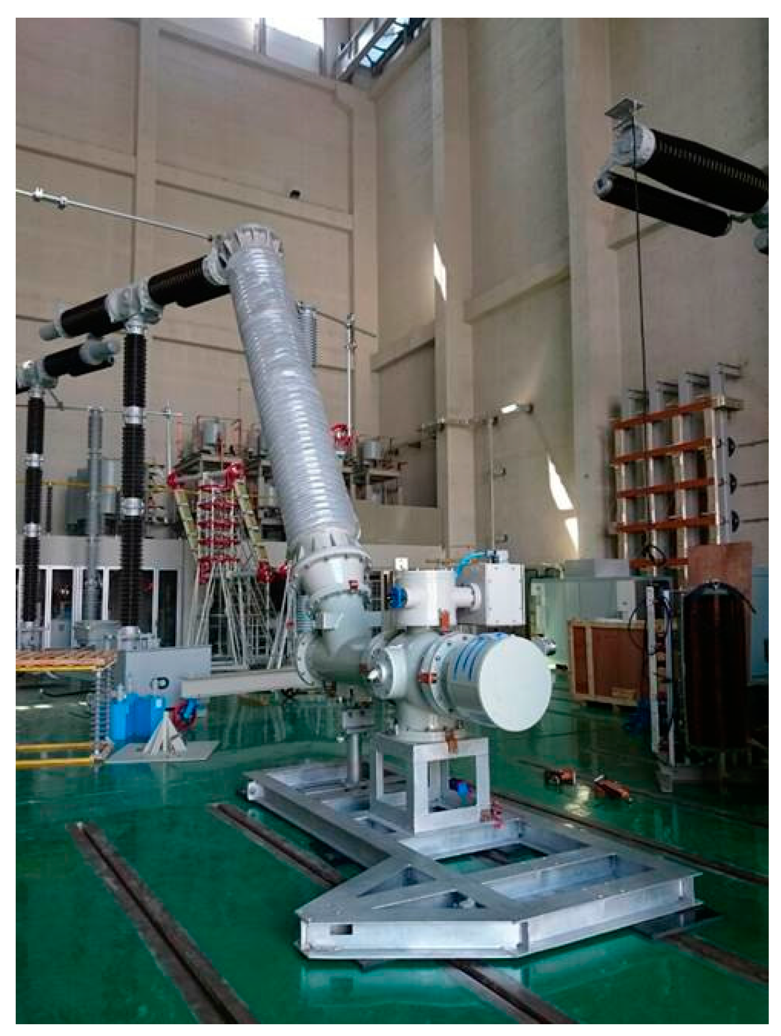
To verify the making performance of the 420 kV 63 kA HSES, development tests were conducted in KERI. Figure 8 shows the test specimen of our 420 kV 63 kA HSES model. As mentioned above, the test was only conducted for a symmetrical test condition; therefore, the HSES earthed at the peak of the applied voltage wave, with a tolerance of −30 electrical degrees to +15 electrical degrees, led to a symmetrical short-circuit current and the longest pre-arcing time [24]. Before the 100% short-circuit current and test voltage were set for the making test, calibration tests were conducted several times by increasing the test currents and voltage levels from 20 to 30%. Moreover, the contact chips and shield, which were damaged by the pre-arc during the calibration tests, had to be replaced for maintenance between Tests #25 and #48.

Table 3. Results of the short-circuit current making test of the high-speed earthing switch.

Test No.	Breakdown Voltage [kV]	Making Current [kArms]	Pre-Arcing Time [ms]	Make Time [ms]
16-0530-020 (#20)	105.6	21.08	2.9	80.1
16-0530-021 (#21)	172.5	20.94	4.9	77.8
16-0530-025 (#25)	221.9	22.90	7.4	74.3
16-0530-048 (#48)	271.7	31.81	7.2	69.4
16-0530-050 (#50)	300.3	60.74	10.8	70.3
16-0530-051 (#51)	332.0	64.65	11.8	69.6

shows the making test results in KERI with test voltages varying from 105.6 kV to 330.3 kV, which is an acceptable value for a tolerance of −30 electrical degrees of 343 kV, and short-circuit currents varying from 20.94 kA to 64.56 kA.

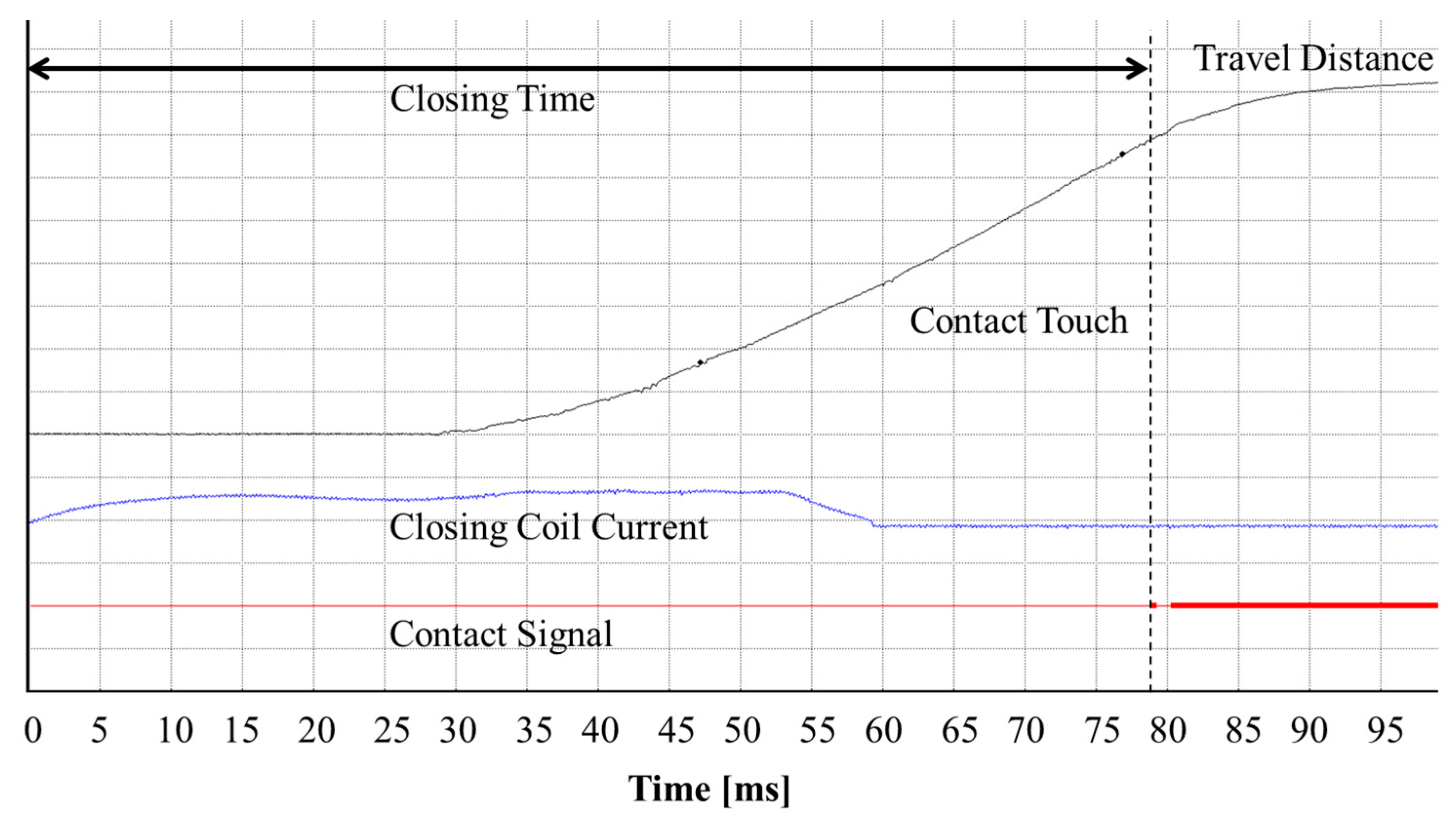
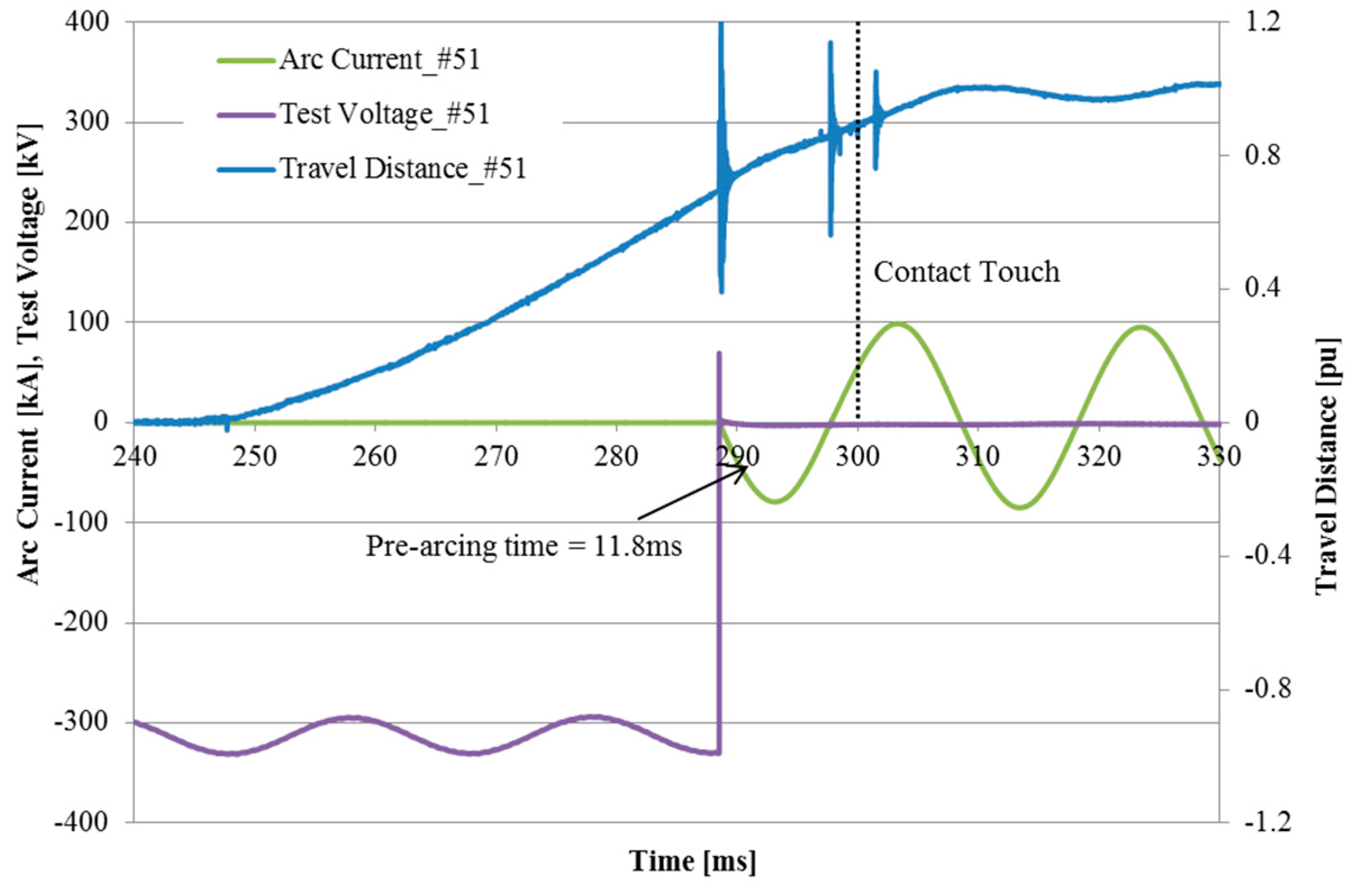
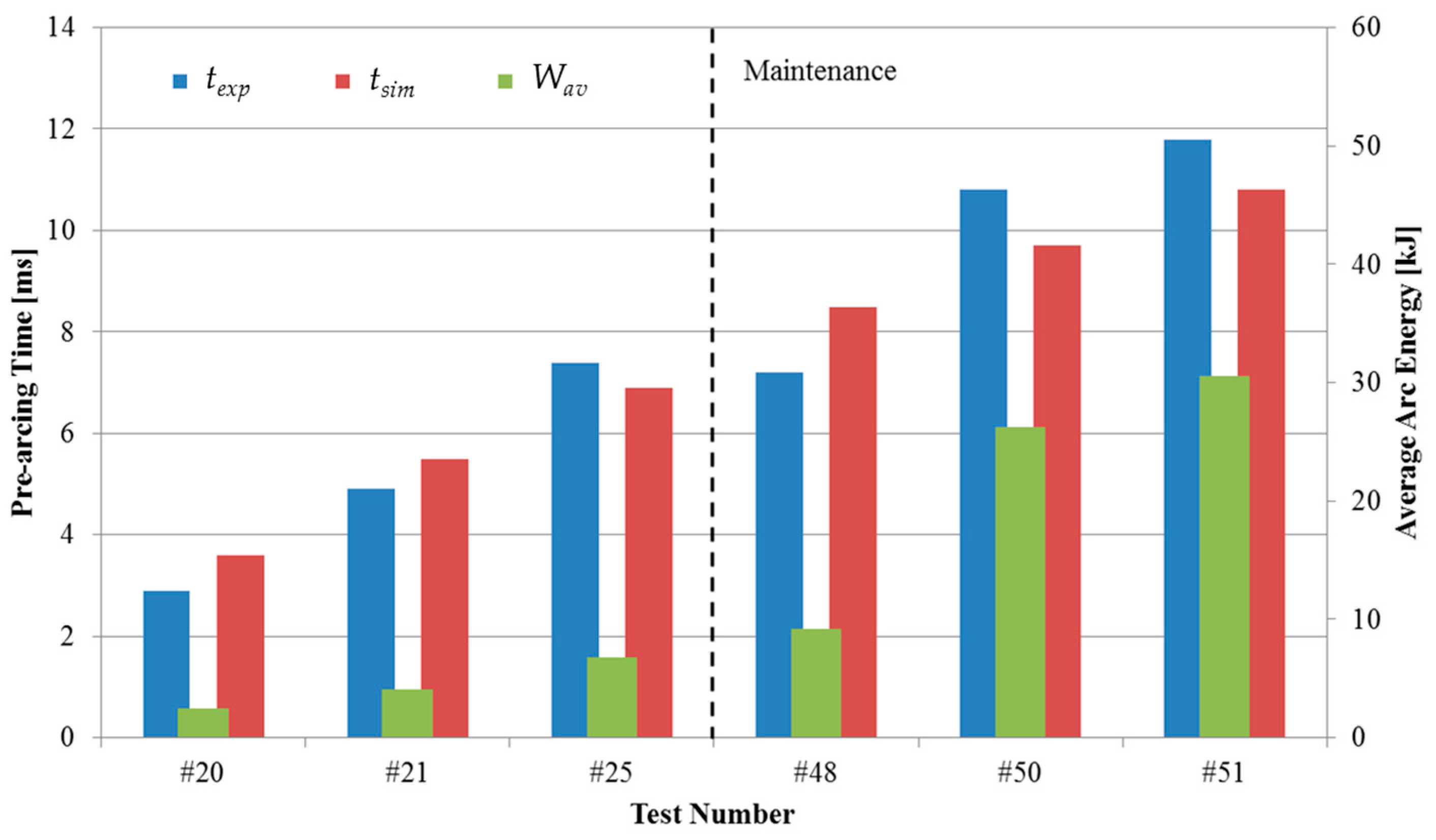
In Table 3, the breakdown voltage indicates the magnitude of the applied voltage at the moment that the pre-arc began. The making current is the root mean square (RMS) value of the applied short-circuit current. In Test #51, the making current reached the intended short-circuit current at over 63 kA for our HSES model. The make time was the interval of time from the initiation of closing coil signal to the moment of pre-arc ignition. By adding the pre-arcing time and make time, the total closing time was calculated. 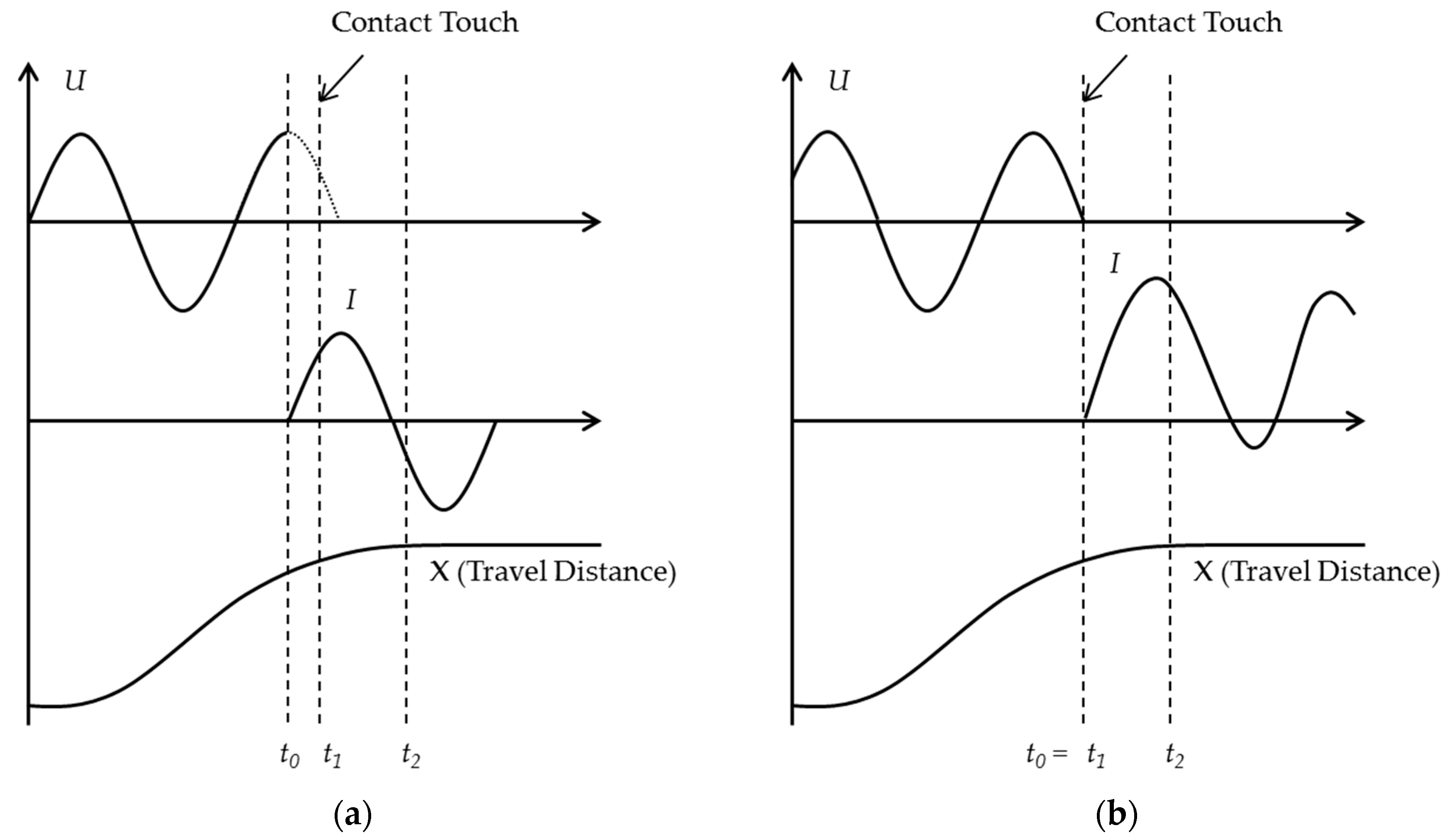The graphs in Figure 9 are the results of the short-circuit current, the test voltage, and travel distance of Test #51. As shown in Figure 9, the closing speed slightly decreased under the on-load condition when approaching the contact touch moment. We presumed that resistive forces from the eddy current damping and/or thermal expansion pressure by arc energy disturbed the closing operation and made it slow, especially during the second half of the operation [27]. Thus, compared to the closing time measuring results under a no-load condition in Section 4, the closing time, the sum of pre-arcing time, and make time, slightly increased. In Test #51 in Figure 9, the pre-arc occurred at the breakdown voltage of 332.0 kV and lasted until the contact touch moment around 11.8 ms.

To compare the test results in Table 3 and the simulation results, the pre-arcing time prediction process introduced in the above section was performed repeatedly in accordance with the breakdown voltages. From the comparison results in Figure 10, although it was confirmed that the prediction model was effectively valid, some difference between the measured pre-arcing times (t_exp) and the predicted pre-arcing times (t_sim) was found. The difference of these results was analyzed as being caused by the dielectric difference between the ideal condition consistent with design drawings and the real experimental condition. For example, in real situations, there are many variables such as metallic particles, eccentricity of moving parts, assembly tolerance, etc. that can deteriorate the dielectric strength between the contacts, especially if the contacts have been damaged by the arc energy from repeated test procedures. If the dielectric strength deteriorated for these reasons, the pre-arcing time could be prolonged.

To analyze the impact of contact damage, the average arc energy (W_av) calculation result of each test condition is shown in Figure 10 using the Cassie arc model introduced in Reference [28]. According to the Cassie arc model, which is suitable for arcs with a high current, the following differential equation for the arc conductance is represented.

$$\frac{1}{g}\frac{dg}{dt}=\frac{1}{\tau }\left(\frac{u_{arc}^2}{U_c^2}-1\right) \mathrm{where} u_{arc}=i_{arc}/g.$$

(12)

In Equation (12), g is the arc conductance; u_arc and i_arc are the arc voltage and current; τ and U_c are the constants that determine the arc characteristic. By comparing the test results and simulation results, the researchers in Reference [28] calculated that τ = 0.000012 and U_c = 80. From the arc voltage in Equation (12) and the arc current measured from our test results, the average arc energy can be calculated as follows:

$$W_{av}=\frac{1}{2}{u}_{arc}^{\max } i_{arc}^{\max } \cos ({\theta }_v-{\theta }_i)t_{arc}.$$

(13)

The average arc energy in Figure 10 is the calculation results from Equation (13), applying the experimental pre-arcing time. When the contact damage caused by the arc energy was small (#20, #21, and #48), the measured pre-arcing times were smaller than the predicted pre-arcing times. In the case of Test #48, although the accumulated arc energy was relatively large, given that the maintenance had been performed and was replaced with new contacts right before the test, the pre-arcing time was measured to be smaller than the predicted result. On the other hand, when the longer pre-arcing time and the higher short-circuit current affected the contacts as the breakdown voltage increased (Tests #50 and #51), the dielectric strength seemed to deteriorate due to the contact damage caused by the accumulated arc energy, so the actual test results of the pre-arcing time were longer than the calculation results. Moreover, as described above, the fact that the closing speed slightly slowed down because of the impact of the arc generation can also achieve longer pre-arcing times of the experimental results than the predicted results. Nevertheless, the prediction results in Figure 10 produced effective outcomes to analyze the performance of the HSES before the laboratory tests. Using this prediction process, the shape of the contacts and closing speed of HSES can be optimized for reducing the pre-arcing time and arc energy.

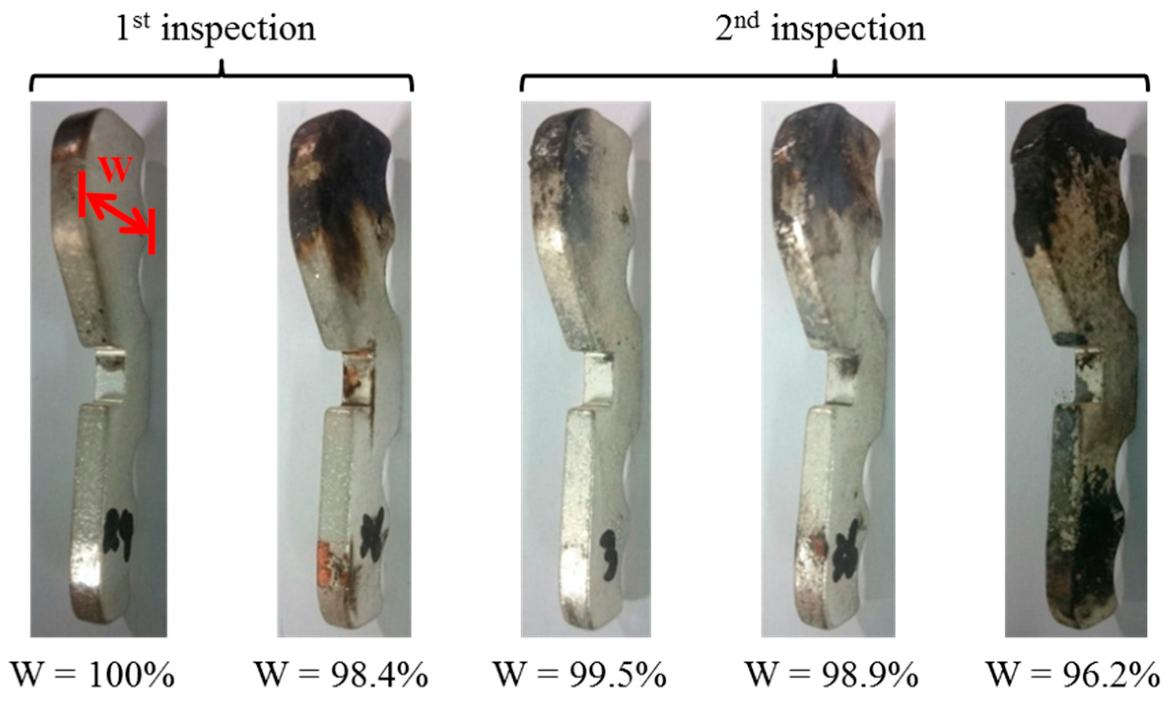
To confirm the impact of the arc energy of the test results in Table 3, the surface condition of the contact chips, contact resistance, and spring tension were inspected twice after Tests #25 and #51. In

Table 4. Surface condition inspections of the contact chips.

Classification	Good	Fair	Poor
Width ratio of contact chip	≥99%	98–99%	≤98%
1st inspection (after Test #25)	44.4%	55.6%	0%
2nd inspection (after Test #51)	16.7%	36.1%	47.2%

, the surface conditions of the contact chips were classified into three groups: “good”, “fair”, and “poor”, according to the ratio of the measured width of each contact chip after inspection to the new one. In Figure 11, the examples of surface condition inspections of the contact chips are shown with the width ratio of each contact chip. As shown in Table 4 and Figure 11, it was found that the contact damage was larger at the second inspection than the first inspection. Especially, in the second inspection, the number of contact chips of the poor set, which was defined as a measured width ratio of the contact chip of less than 98%, increased to 47.2%. This result shows that the arc energy during the second period after maintenance was relatively larger than the first period before maintenance.

The inspection results of the contact resistance are shown in

Table 5. Contact resistance inspections.

No.	Initial	1st Inspection	2nd Inspection
1	6.90 μΩ	26.60 μΩ	29.50 μΩ
2	6.80 μΩ	26.30 μΩ	28.20 μΩ
3	6.80 μΩ	26.10 μΩ	27.60 μΩ
Average	6.83 μΩ	26.33 μΩ	28.43 μΩ
Ratio of average	1	3.85	4.16

. In comparison to the initial contact resistance, the average contact resistance of the first inspection increased 3.85-fold while that of the second inspection increased 4.16-fold. These contact resistance measurements also revealed that the contact chips were damaged more during the second period tests compared to the first period tests, but the current-carrying performance was still maintained after the second inspection. Therefore, the HSES after finishing the whole test sequence could still keep its current-carrying performance.

It is important that the holding springs of the contact chips were not deformed by the arc energy during the making test. If they lose their tension, the contact force becomes weak, leading to an increase in contact resistance. In the HSES, quad springs encircle the contact chips so that they are tightened to decrease the contact resistance. Fortunately, in the first inspection, the quad springs had been deformed slightly because of the low arc energy. The top string, however, had lost its tension by approximately 5% in the second inspection as full-current arc energy was applied. The top spring was slightly deformed and bent in the naked eye. Nevertheless, the contact resistance of the second inspection did not increase much more than expected, as the tensions in the other three springs almost retained their initial states. This meant that the current-carrying performance of the HSES did not degrade after the making test. In

Table 6. Holding spring tension inspections.

Elongation Length	Inspection No.	Initial Value	Spring 1	Spring 2	Spring 3	Spring 4
40 mm (N)	1st	70.41	68.84	72.96	76.10	70.41
	2nd	70.41	70.41	76.88	77.47	72.96
55 mm (N)	1st	117.48	115.33	119.44	122.98	116.90
	2nd	117.48	115.33	123.37	123.76	118.86
Spring Constant (N/mm)	1st	3.138	3.100	3.100	3.128	3.100
	2nd	3.138	2.991	3.100	3.089	3.060

, we arranged the results of the spring-tension inspections (which were measured twice) along with the longitudinal elongations. The spring constants in Table 6 were calculated via Hooke’s law using the results of the spring-tension inspections [26].

6. Conclusions

Predicting the insulation performance is very important in GIS technology. This paper investigated the insulation performance of HSES during a making test. For the HSES making test, calculating the pre-arcing time before conducting high-power tests was extremely valuable in saving development costs. In this paper, we introduced a method to predict the pre-arcing times in HSES using the streamer discharge theory and electric field simulations. Using this method, the pre-arcing time of a 420 kV 63 kA HSES making test was predicted and compared with the test results from a high-power laboratory. We found that this prediction technology produced effective outcomes regarding the success or failure during the tests. This process can be extended to pre-arcing time prediction for other parts such as disconnecting switches (DS) or circuit breakers (CB) in GIS.

The pre-arcing time prediction process can be summarized as follows:

• The average breakdown electric field strength was calculated based on the streamer discharge theory, considering the gas pressure, harmonic radius of contacts, distance between electrodes, etc.
• The real travel distance data from switches (HSES, DS, and CB) were obtained by measuring the operating characteristics.
• The two-dimensional or three-dimensional electric field distributions of the test objects were analyzed using finite element method analysis tools in accordance with the real travel distance data.
• The results of the calculated average breakdown electric field strength and peak value of the simulated electric field distribution were compared.
• The breakdown factor λ was calculated and the time when this factor became greater than 1 was found.