1. Introduction
Over the past decades, wind energy has been widely regarded as an effective energy solution to reducing CO
2 emissions and producing sustainable energy because of its technology maturity and improved cost competitiveness. One of the key priorities identified by the wind industry is to reduce costs in the operation and maintenance of wind turbines, which currently accounts for 18% of the cost of offshore energy [
1]. A cost-effective operation of the wind farm is therefore crucial due to the fierce competition in the global sustainable energy market. Monitoring of the operating conditions of the wind turbines has been considered as an effective method to enhance the reliability of wind turbines and implement cost-effective maintenance. Clearly, it is essential to develop effective CM techniques for wind turbines [
1,
2,
3] to provide information regarding the past and current conditions of the turbines, and to enable the optimal scheduling of maintenance tasks [
4].
From surveys concerning the reliability of the wind turbines, faults caused by the drivetrain system account for over 20% of total faults and contribute to approximately 30% of the downtime of doubly-fed induction generator (DFIG)-based wind turbines [
5,
6]. Thus, studies about fault diagnosis of the drivetrain system are necessary.
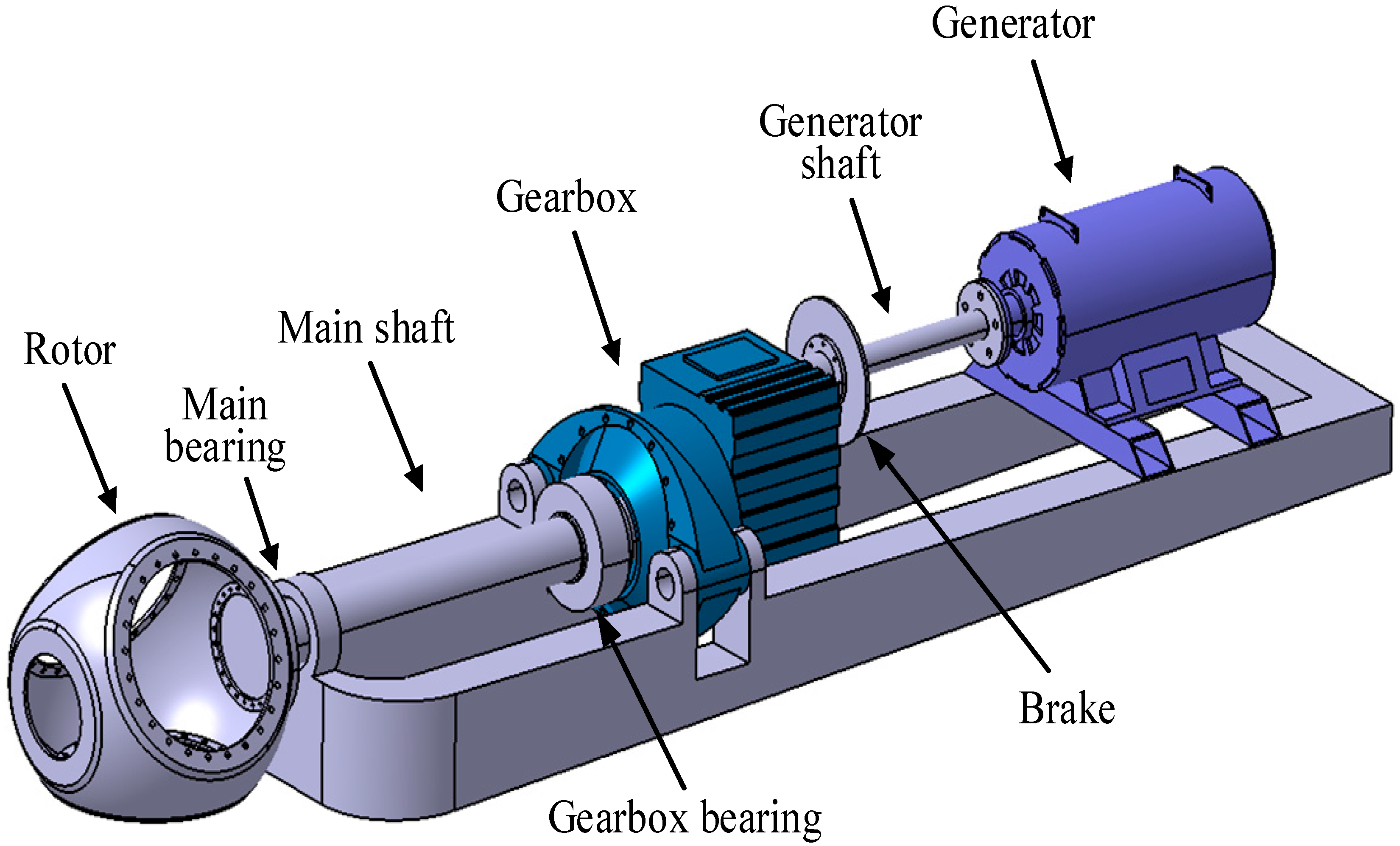
Figure 1 shows a typical drivetrain system in a DFIG wind turbine that contains hub, main bearing, main shaft, gearbox, brake, generator shaft and generator. The main function of drivetrain system is to transmit kinetic energy from the turbine rotor to the electric generator by adjusting rotational speed and torque.
For the mechanical transmission system, monitoring and analysis of the vibration signals have been proven very effective, as it is easy to obtain the fault signature of a specific component in the frequency or time-frequency domains. However, it is difficult to obtain accurate vibration signals in the wind turbine under varying speed operation. Furthermore, condition monitoring based on vibration signals is a kind of component-specific technique, which lacks providing an inherent relationship between different subsystems [
7]. For example, variable speed wind turbines have the function of maximum power point tracking that optimizes performance in relation to time changing wind speed. This means the rotor, gearbox and generator rotational speed may change significantly and frequently during operation. Due to the significant rotational speed change, the vibration frequency bandwidth varies, which may cause difficulties in locating the exact location of the fault.
Acoustic emission (AE) is another effective method that can be applied in condition monitoring of the wind turbine [
8]. When materials bear external strain or stress, they may generate sound waves called AE. Even a tiny structural change will make AE signals to be excited, meaning that AE signal is very suitable to be applied to detect incipient structure defect and monitor its development. For wind turbines, AE signals are generally used for fault detection of the blade, gearbox, bearing, and generator. Compared with vibration signals, AE signals have high signal-to-noise ratio, which means that AE signals can be applied in high-noise environments. However, AE technique also has its own disadvantages. To monitor subsystems of the wind turbine, it is necessary to install a large number of AE sensors, and each sensor requires an independent data acquisition system for signal sensing, processing and transferring, which increases the cost and complexity of the condition monitoring system.
Monitoring techniques based on temperature signals have been developed for fault diagnosis of gearboxes, generators, and power converters. Furthermore, temperature signals can also provide key information on the health condition of mechanical transmission system in wind turbines [
9,
10,
11]. However, in previous work, the relationship between the temperature rise and the operating power has not been considered yet. Although the same temperature change can be observed whilst under different operating power, its effect on the indicative damage of the drivetrain system might be different. For example, a temperature anomaly will cause different working efficiency for the drivetrain system when working at full power and half power conditions. A working efficiency decline as low as to 0.34% for each gear stage would lead to 10 KW power loss in a 1 MW wind turbine [
12,
13,
14]. In [
15], the relationship between the gearbox temperature and power generation is illustrated; however, it does not consider correcting temperature changes under different power output condition for drivetrain condition monitoring.
A new data-driven model-based method is proposed in this paper for estimating the health condition of the drivetrain in wind turbines. The model to predict output values is built based on the OS-ELM algorithm [
16]. The residual signal is then obtained by comparing the predicted values with those from measurements. Compared with other artificial intelligence (AI) methods, such as artificial neural networks (ANNs) [
17], support vector machines (SVMs) [
18], OS-ELM has a faster training speed and a better generalization performance [
19]. The residual signal produced is then further assessed by the physical kinetic energy correction model of the drivetrain, which evaluates the degree of faults by investigating the relationship between the temperature rise and power output. Finally, the Bonferroni method, a cost-effective method used to counteract the problem of multiple comparisons, is used to adjust and assess the health condition of the drivetrain. Although a physical model was proposed and applied to investigate relationships between temperature, efficiency, rotational speed and power output in [
15], one major contribution of this paper is that the temperature rise is normalized at the rated power output, thus providing a more sensitive diagnosis. This paper also assesses the health condition using multivariate data analysis by taking into account both the independence of variables and the relationship among variables, which is more appropriate when modeling a practical process than the univariate analysis. Essentially, a wind turbine is a complex multivariate system, resulting in strong coupling among variables.
The remainder of this paper is organized as follows. Working principle of the online sequential extreme learning machine is presented in
Section 2.
Section 3 describes the physical kinetic energy correction model for the wind turbine drivetrain while
Section 4 calculates the health condition of gearbox based on the Bonferroni interval. A case study using SCADA (Supervisory Control and Data Acquisition) data is then performed and the results are shown and discussed in
Section 5.
Section 6 contains conclusions and suggestions for further research.
2. Online Sequential Extreme Learning Machine
Extreme learning machine (ELM) algorithm was first proposed by Huang [
20] for single hidden layer feed forward neural networks (SLFNs). Compared with other traditional supervised batch learning algorithms in ANNs, ELM algorithm has the advantages of faster learning and better generalization capability [
21,
22,
23,
24]. However, the ELM algorithm assumes that all training data are available before the training begins. In real cases, this assumption cannot always be satisfied, as data are available for training on a chunk-by-chunk or one-by-one basis. Thus, this paper considers using a novel sequential extreme learning machine due to its advantages below.
- (1)
OS-ELM learning algorithm can receive the training data sequentially, i.e., arriving chunk-by-chunk or one-by-one.
- (2)
At any time, only newly arriving data are used as training data and transferred to the learning algorithm.
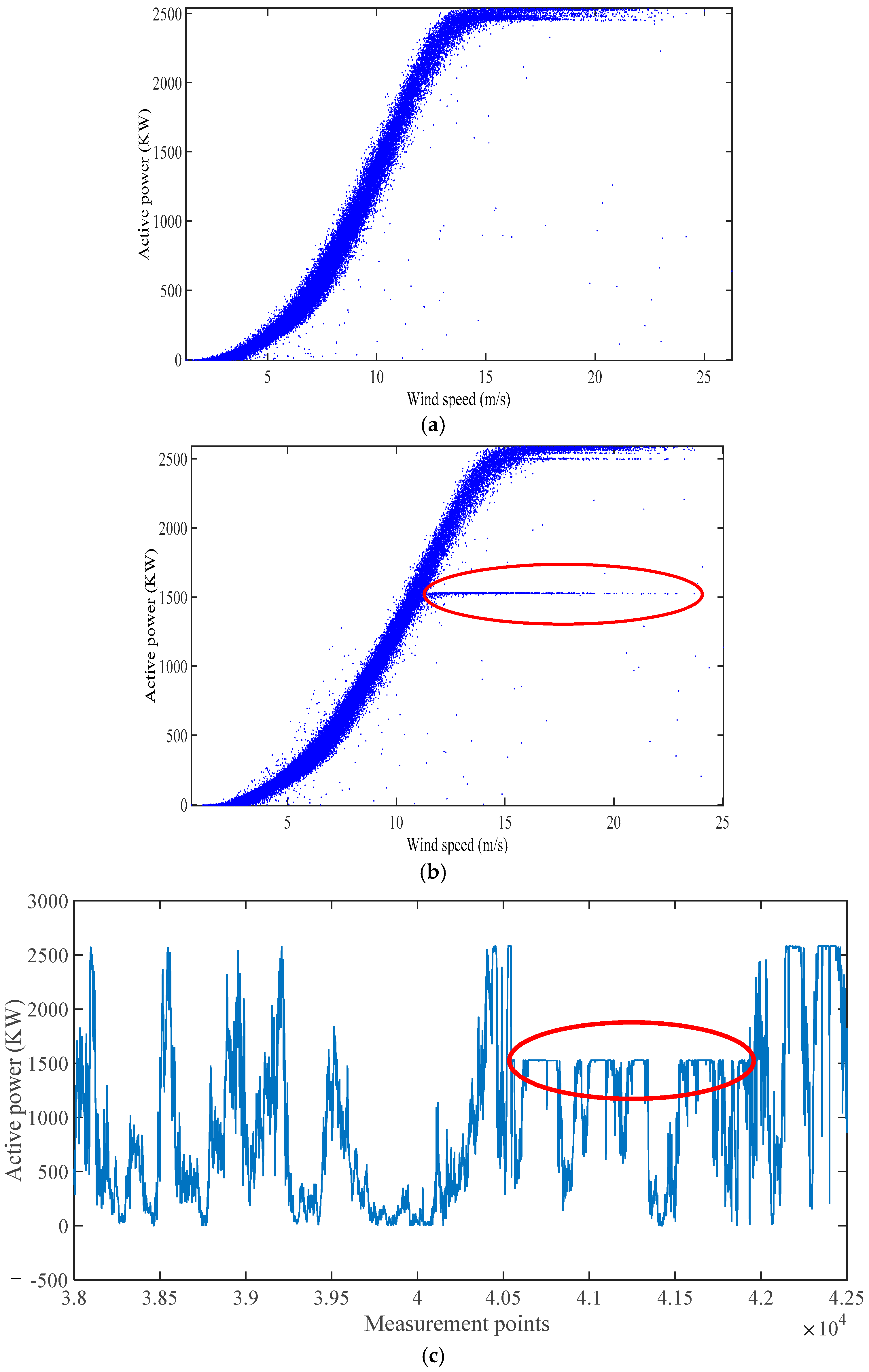
Thus, the application of OS-ELM algorithm is very suitable for condition monitoring of wind turbines. Nowadays, the operation of wind turbine follows the power curve designed by the wind turbine manufacturer. As an example, a normal power curve of turbines from SCADA data is illustrated in
Figure 2a; turbine power varies cubically with wind speed, and wind speed varies continuously on time-scales. When the wind speed is lower than the cut-in speed (4 m/s in this case), the turbine does not produce any power because the rotor torque is too low. When the wind speed is above the cut-out speed (25 m/s in this case), the turbine does not produce any power either because it has to be shut down to protect it from overloading. If the wind speed is above the rated wind speed (15 m/s in this case) but below the cut-out speed, the turbine’s output power is capped at the rated power.
The normal power curve can represent the operation performance of a fault-free wind turbine. The change of operation performance, i.e., the change of the power curve, may indicate the onset of a turbine fault. The power curve of a wind turbine, as shown in
Figure 2b, is an example of abnormal operations. In this case, the wind turbine reduces to half of its rated power output, as shown in the red circle in
Figure 2b and wind power time series data in
Figure 2c, to prevent the development of more serious problems. Compared to an immediate shut-down once the fault is detected, the operation of the turbine by reducing power output would reduce the dynamic mechanical loads experienced by the turbine structure, whilst still maintaining its operation.
When the operation performance is changed, new training data should be refreshed into the prediction model to fit the new operation scenarios. Thus, the advantages of OS-ELM algorithm are able to update training data resulting from the new operation scenarios of the wind turbine. A full description of the OS-ELM algorithm is given as follows.
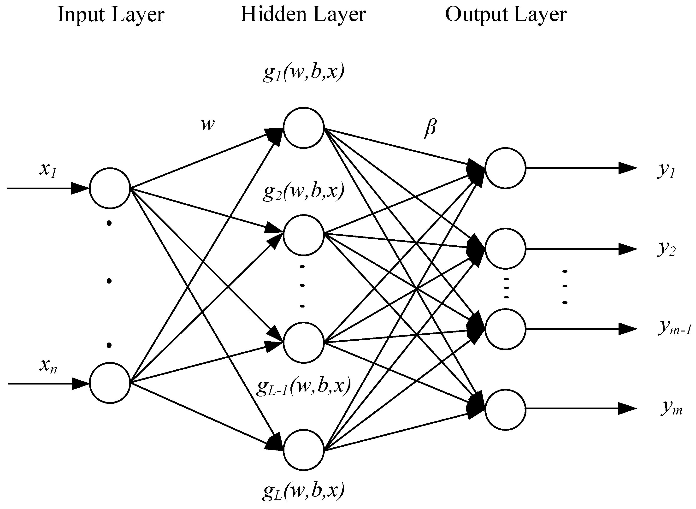
The schematic diagram of a single hidden-layer feed forward neural network is shown in
Figure 3, which consists of an input layer, a hidden layer and an output layer. It assumes that the input layer and the hidden layer have n and L neurons, respectively, while the output layer has m neurons;
x1,
x2, …,
xn and
y1,
y2, …,
ym are input and output signals, respectively.
If there exists an ELM with
L neurons in the hidden layer and an activation function
g(.) can approximate the
N samples with zero error, the output matrix
M of ELM between inputs nodes and outputs nodes can be represented by
where
is the weight vector between the
ith hidden node and input nodes;
is output weight vector connecting the
ith hidden node and output nodes;
is the
jth input samples; and
represents the bias of the hidden layer matrix.
For simplicity, Equation (1) can be compactly described as,
where
is the transpose matrix of
M and
H is the output matrix of the hidden layer of the ELM. The matrix
H can be expressed as,
When the input weight matrix
w and the hidden layer bias matrix
b are initialized, the hidden layer output matrix
H can be uniquely determined. The output weight matrix
β can be calculated by minimizing the error function as follow,
During this process, the input weight matrix
w and the hidden layer bias matrix
b do not need to be changed and the solution can be expressed,
The matrix is the generalized Moore-Penrose inverse of the matrix H, which can be found using the singular value decomposition method.
To make ELM online sequential,
can be transferred as follows:
Suppose the training data has two sets; one is the chunk of initial training data
N0 and another is the chunk of new training data
N1. Then, the Equation (5) can be updated to Equation (8) by minimizing the error function between two moments, where
and
are the output matrix of the hidden layer and the output matrix for the initial training data
N0, while
and
are the output matrix of the hidden layer and the output matrix for first chunk of training data
N1.
The output weight matrix
β that considers both initial block of training data
N0 and block of training data received in the next moment
N1 becomes
where
Therefore, the output weight matrix
for the 1st chunk of training data
N1 is updated. Suppose
is the output weight matrix for the chunk of initial training data
N0, then
As mentioned above, when a chunk of data arrives at step
K + 1, the parameters are updated as follows:
Using
, the equation for
can be updated
The output weight matrix
at step
K + 1 therefore becomes
Hence, this sequential ELM algorithm has the ability of achieving an online training in real time, if the sampling speed for updated training data is quick enough. However, it is worth noting that, in this paper, the main purpose of using OS-ELM is to achieve updated training data to ensure that the model is adapted to accommodate different operational behaviors of the wind turbines encountered during their operations. Real time online training capacity of the method is not considered in the paper. In this paper, one-year historical data are used as initial data to train initial weights. When new scene data are available, the new dataset is then transmitted to OS-ELM model to update the weights.
In our study, the updating duration is one month and the length of the data to be used is around between 4320 and 4464 points for each parameters depending on the calendar month; more information about data can be seen in the later
Section 5.1. It is worth emphasizing that the data obtained from the fault-free turbine are selected for model training. Then, the data gained from a turbine with system aging only and a faulty turbine are used as the input data of the model to predict their monitoring variable output. Consequently, the established model can identify both the aging and faulty wind turbines.
As verified in our previous work [
24], the ELM can learn much faster than the traditional back propagation (BP) neural network while still achieving similar model fit performance.
3. Physical Kinetic Energy Correction Model
As a key component of DFIG turbine drivetrain, the gearbox is used because turbine rotor cannot reach synchronous speed that satisfies the operating condition of DFIG generator. The use of gearbox is to transmit kinetic energy from the turbine rotor to the DFIG electric generator through the drivetrain system. The CM of temperature signal is a proven method to diagnose the faults and predict the residual life of the drivetrain system. Traditionally, a same threshold is applied to temperature monitoring regardless of the operating power, which means the same weight is assigned for the temperature change contributing to the damage of gearbox. However, the operating power could have a significant impact on the temperature changes; therefore, its effect on the temperature changes should be weighted differently.
Supposing σ is the drivetrain system efficiency, E is the input kinetic energy from the rotor to the drivetrain, P is the output kinetic energy from gearbox to generator, then E = 1/σ × P.
Based on the first law of thermodynamics, we can have
where
Q represents the heat loss of gearbox, which leads to the temperature rise of drivetrain. If
is the compound heat transfer coefficient, the relationship between the heat loss of drivetrain
Q and the gearbox temperature rise
can be described by
Substituting Equation (17) into Equation (16) gives
In the ideal conditions, the compound heat-transfer coefficient
is considered as constant.
Figure 4 illustrates an example of the relationship between temperature rise and efficiency change of the drivetrain at different operating power outputs for a 2.5 MW wind turbine. As can be seen from the figure, the efficiency change varies at different power outputs. This implies that a fault occurring in drivetrain will lead to an increase in
in response to a reduction of efficiency
if the same power output is to be maintained. The higher the operating power output is, the smaller the efficiency varies under the same temperature change
. This also means, although the faults may cause a same value of
, their effects on the level of damage of drivetrain differs if the power output is different.
Consequently, a temperature correction method should be considered. In our study, the temperature change is firstly obtained from the ELM model in response to the power output gained from SCADA data, and then the corresponding efficiency is calculated by using Equation (18). The temperature is further corrected to the value when the turbine is operating at the full power at the given efficiency. All the temperature changes at different power outputs are thus finally normalized to the value at the rated power output.
4. Estimating the Health Condition
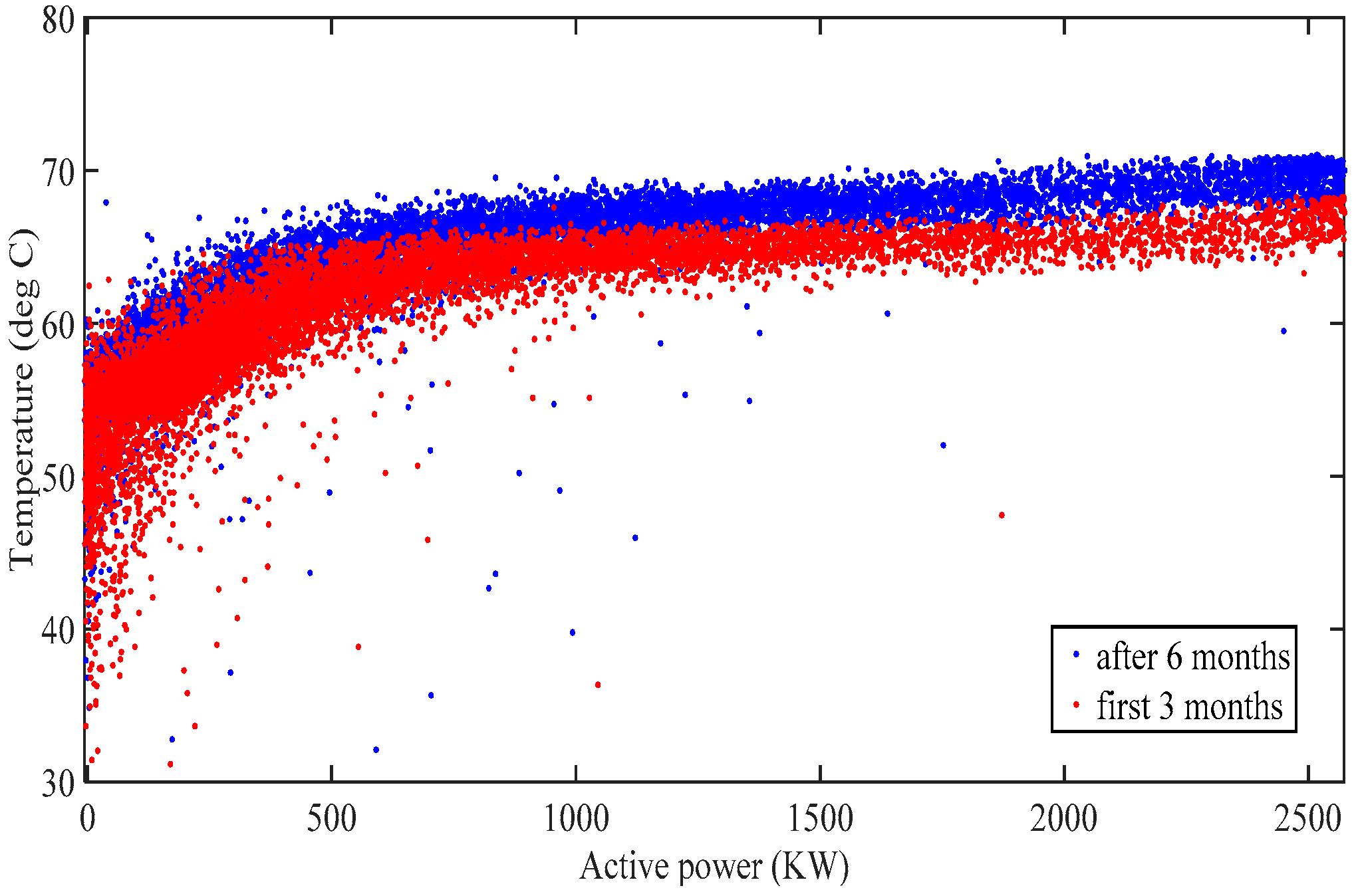
The residual signals obtained from prediction model are now processed by the energy correction model. For the gearbox, its bearing temperature rise can be caused by either the gearbox aging or a potential fault or a failure.
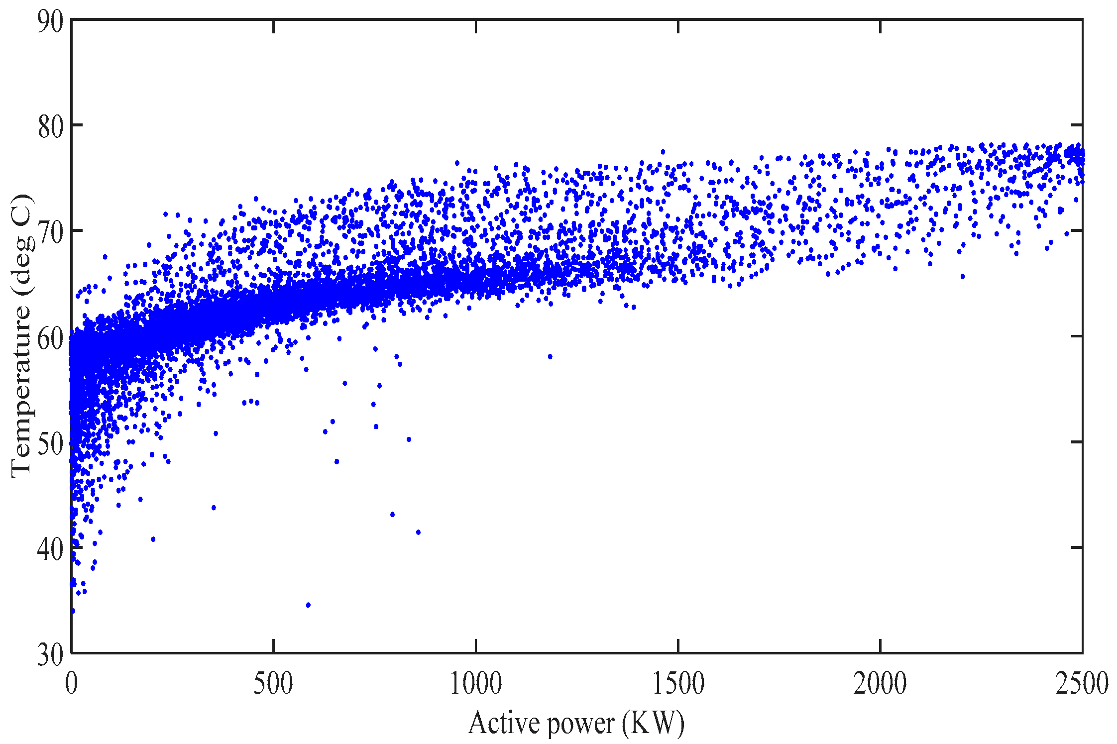
Figure 5 shows an example of temperature curve of gearbox bearing due to system aging in wind turbine. The temperature curve in red shows the trend of temperature rise with active power in the wind turbine due to system aging only during first three months of one year. Temperature rises with increasing active power output. The temperature curve after six months of operation is also shown in the figure with blue color; apparently, temperature increases after the turbine operates for a period. An example of temperature rise due to a fault of the gearbox is shown in
Figure 6. In this case, the temperature actually deviates from the curve randomly, indicating the onset of a fault. The fault is identified after checking the event logs recording user activities, exceptions and alarms in the SCADA system, which is related to the gearbox cooling system.
In the model-based CM systems, faults can be diagnosed by comparing the difference between the actually measured signal and the predicted value from the sequential extreme learning machine algorithm. Although a method relying on residual signals alone can detect faults effectively, it is not able to evaluate accurately the significance about the failure of components. Furthermore, the drivetrain in a wind turbine is generally composed of several components, which are, specifically, gears, bearings and the cooling system (usually oil cooling). Clearly, it would be desirable to use a more appropriate method in order to identify the health condition of the drivetrain by considering relationship between different components.
The estimation of system performance by using Hotelling’s T-square, as described in Equation (19), has been proven to be effective in [
25], where the method was used to achieve multivariate failure mode analysis of electronics. The method can provide the global information of deviation level in wind turbines. Confidence intervals for the Hotelling’s T-square method can be computed using Equation (20) and utilized to estimate deviation level for each variable.
where
indicates a set of variables, for example, the temperatures of gearbox bearing
u1, gearbox oil
u2, and drivetrain main bearing
u3 in this study. The
, where
represents the mean value of the measurement parameter
. The distribution
is a
F distribution used in statistics;
N is the number of the samples for each measurement parameter; the parameter
p is the number of variables;
is the covariance matrix of
U;
is diagonal value in the covariance matrix. In Equation (20),
represents the critical value for the
F distribution; when
is determined, the value of
can be found from the
F distribution table [
26] and the confidence interval is thus determined. It is worth noting that
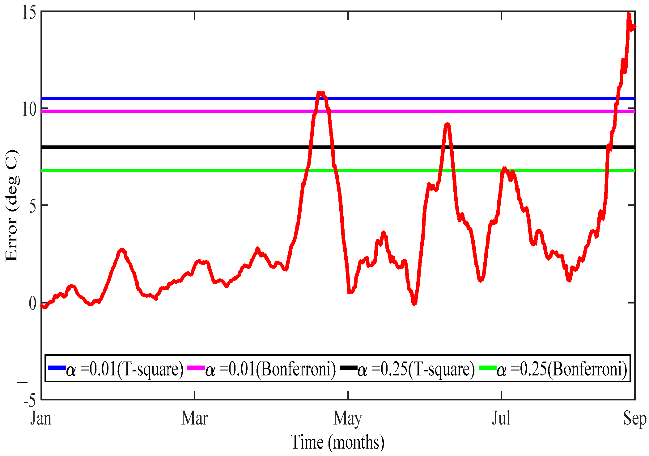
indicates probability of occurrence of the residual signal values. If
< 0.01, the monitoring data are considered to indicate a fault in the component [
7], while, if
is larger than a particular value which can be application dependent, the component can be in a debilitating condition. In this case study,
= 0.25 is selected as a threshold value for debilitating condition.
Despite of the global effect the above confidence interval demonstrates, the method lacks the ability to provide details concerning the effect of individual components on the overall operational conditions. Instead, Bonferroni intervals simply focuses on the means for each of the individual variables themselves, thereby enabling to build a more accurate confidence interval range [
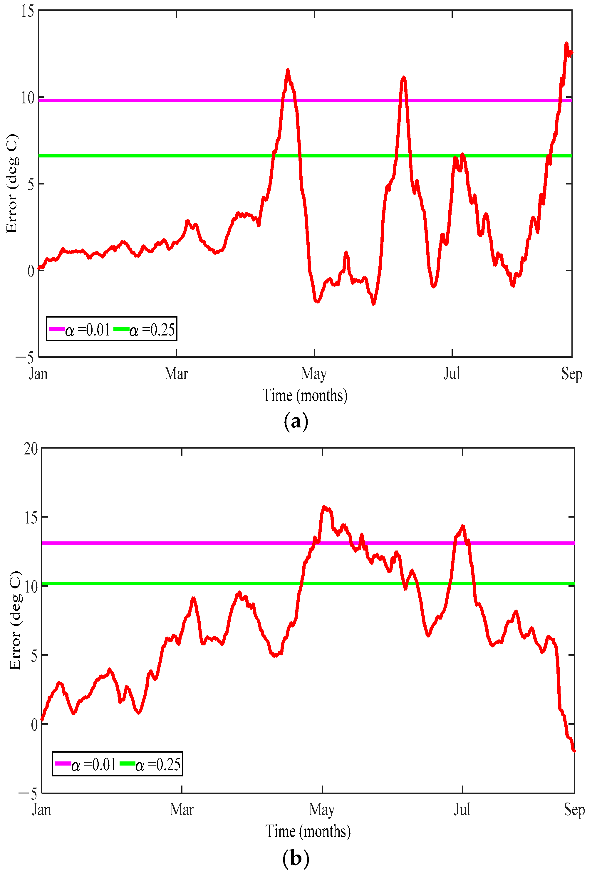
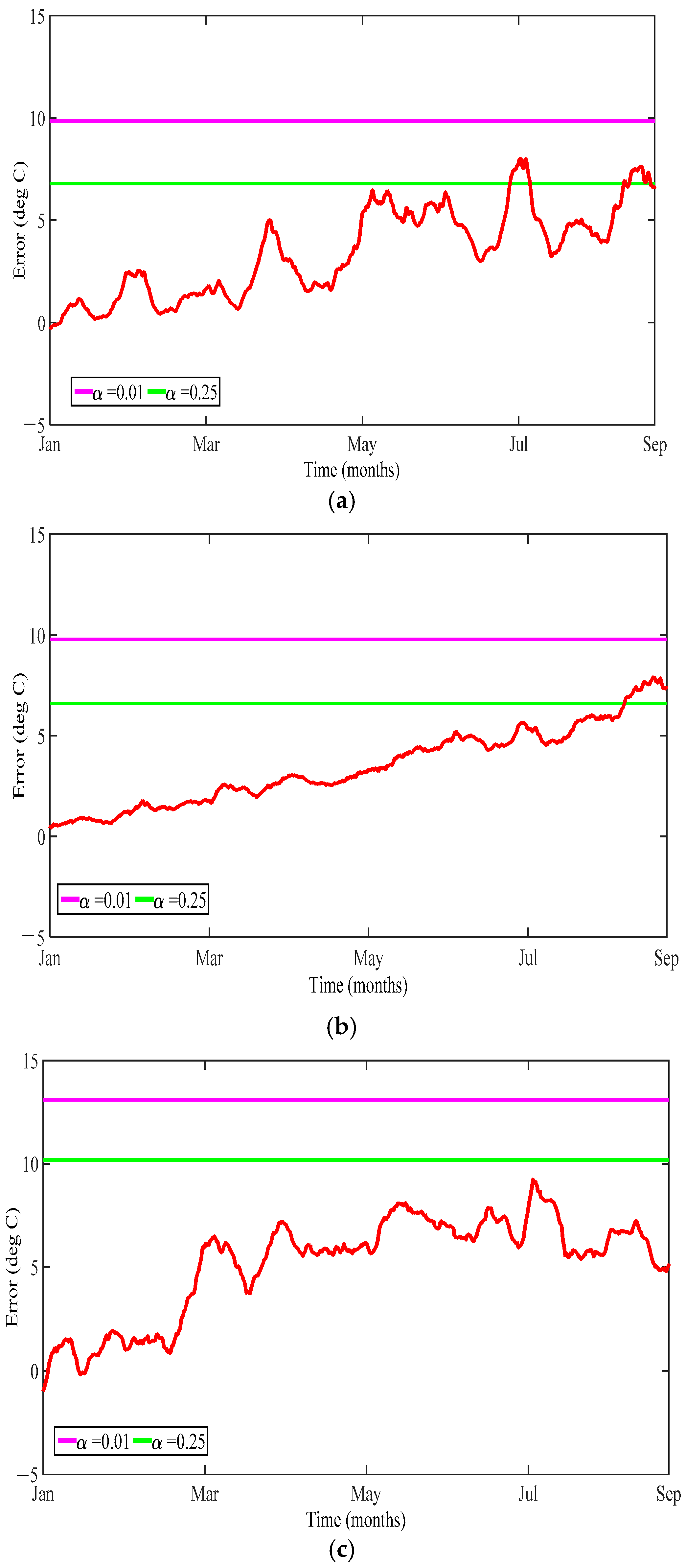
26]. Thus, Bonferroni intervals, as described in Equation (21), are applied in this study.
The distribution is a t distribution used in statistics and the value of can be found from a t distribution table. In our study, the value of residual signal after processing with the energy correction model is considered as a fault if the value is higher than . Meanwhile, is defined as the threshold value for debilitating condition.


