1. Introduction
Permanent magnet (PM) machines are widely used in motion applications with high power densities, e.g., pumps, compressors and fans. In particular, PM machine drives at high speed have demonstrated advantages in applications with a size constraint [
1,
2,
3]. Among these applications, machine drives without position sensors are preferred, since the sensor installation reduces the torque density per unit volume and increases the overall drive size [
4,
5,
6]. To reduce the cost and volume of the device, a single current sensor drive is proposed in [
7] which can reconstruct three phase currents based on the measurement of DC-link current. In [
8], several sensorless drives for PM machines have been reviewed. By using the spatial signal in the machine itself, position sensorless drives are able to perform field-oriented control (FOC) without separate position sensors [
8,
9,
10].
Position sensorless drives can be categorized as saliency-based drives [
11,
12] and electromotive force (EMF) based drives [
13,
14,
15,
16,
17,
18] dependent on the spatial signal in a machine. For operation at zero and low speed, position estimation using the spatial signal in rotor saliencies is preferred because all EMF-based drives eventually fail at very low speed [
11,
12,
19]. Reference [
17] proposed an improved initial rotor position estimation for low-salient machines. By contrast with conventional methods, polarity detection is more accurate, by filtering the spatial harmonics in inductances. In addition, [
20] addresses the sensorless estimation of interior PM machines using rotor saliency and the adaptive filter. The position signal is obtained directly from current ripples instead of saliency signal demodulation. It can be concluded that the signal is better due to the adjustable controller bandwidth. By contrast, beyond 10% rated speed position estimation using the spatial signal in EMF voltages results in a comparable performance to saliency-based drives [
14,
15,
20]. Under this effect, EMF-based position estimation methods are preferred at high speed for the sensorless drive, because no voltage injection is required to fully utilize the DC bus voltage.
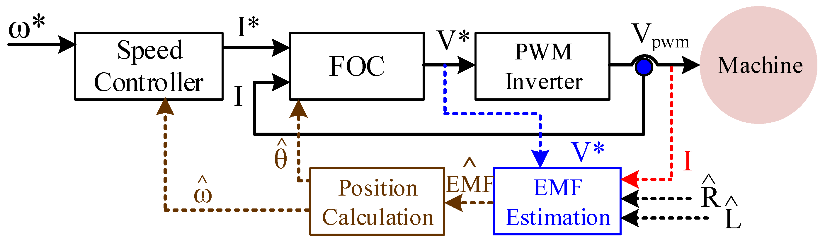
For EMF-based drives, the EMF voltage is estimated according to the voltage and current relationship with the knowledge of machine resistance and inductance. The rotor position is then calculated by obtaining the spatial signal in the estimated EMF voltage. The overall EMF-based drive system is shown in
Figure 1. Considering the EMF estimation algorithm denoted by the blue block, EMF voltage can be estimated from either the open-loop calculation based on the machine model [
14,
21,
22,
23,
24,
25] or the closed-loop state estimation using observer technologies [
26,
27,
28,
29,
30,
31,
32]. Open-loop methods directly calculate EMF voltage based on the machine model. The estimation accuracy can be influenced by current noises as well as resistance and inductance variation due to the open-loop calculation. By contrast, closed-loop methods estimate EMF using the current observer with machine parameters. Because of the observer filter property, the influence of current noises can be negligible. Reference [
18] improves the conventional observer estimation by compensating the DC offset error resulting from the A/D converter, op-amp gain and voltage sensor gain deviation. A nonlinear PLL is also added to improve the observer estimation performance [
33]. A speed controller is also proposed to achieve a better sensorless dynamic performance. Reference [
34] proposed an active damping control for the sensorless drive of an interior PM machine. The proposed method reduces the influence of parameter errors by increasing the equivalent damping of the drive system. In addition, [
35] developed an adaptive torque estimation for PM machines considering the inductance parameter variation. However, the accuracy of EMF estimation is still sensitive to the parameter variation. It is also noteworthy that the observer estimation bandwidth strongly depends on the signal-to-noise ratio of machine currents. At high speed, due to the limited bandwidth, EMF estimation in the observer might result in phase lag, which degrades the sensorless drive performance.
EMF voltages can be estimated based on AC signals in the stator-referred stationary frame [
26,
27] or DC signals in the rotor synchronous frame [
28,
29]. For AC EMF voltages, the rotor position is calculated based on the arctangent function [
27] or the PLL [
20,
26,
33]. On the other hand, for DC EMF voltages, the rotor position can only be obtained from the PLL. Considering the position estimation using PLL, a small-signal approximation is assumed where the estimated position
is almost equal to the actual position
. Under this effect, the feedback position signal sin(
−
) can be simplified by
−
for the closed-loop regulation [
9,
10,
13,
36]. Unfortunately, at high speed, the ratio of sampling frequency,
, over the rotor operating frequency,
, is low due to the limitation on the inverter switching frequency. Considering the discretized effect at low
, the assumption where sin(
−
) ≈
−
might not be valid, leading to stability issues on EMF-based drives.
This paper improves the PM machine sensorless drive specifically for high-speed operation. As reported in [
37], a discrete-time machine model is implemented to estimate EMF voltages considering discretized effects at low
. The high-speed drive performance can be improved by including the zero-order-hold (ZOH) reflected voltage delay in the EMF estimation. This paper extends [
37] in order to further enhance the sensorless position estimation using discretized EMF voltages. On that basis, a PLL cascaded with an arctangent function is used to remove the small-signal approximation at high speed. By using the arctangent calculation, the dynamic operation of a sensorless drive can be maintained even at high speed with low
. By cascading the PLL after the arctangent calculation, the position estimation error is reduced due to the filter property in the PLL [
20,
33]. In addition, compared to existing estimation methods receiving only the spatial signal from d-axis EMF [
9,
10,
13,
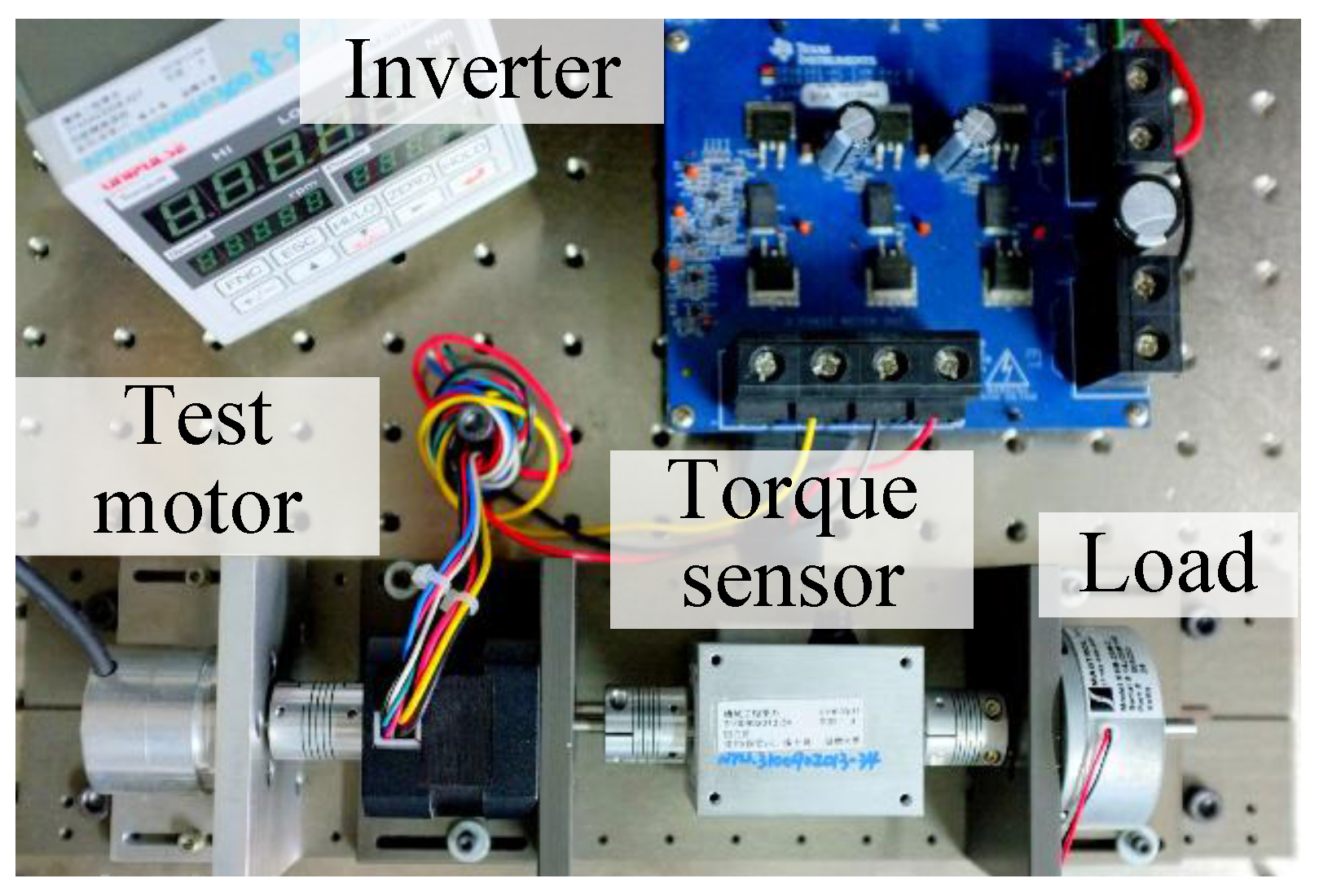
36], the proposed position estimation uses spatial signals from both the d- and q-axis EMF voltage. At high speed, another advantage is the reduced parameter sensitivity on the EMF-based position estimation. In this paper, a 126-W 8-pole surface PM machine is experimentally tested. By applying the discrete-time EMF estimation and modified PLL, the drive can operate at the speed of 36 krpm under 50% step load with only 4.2 sampling points per electrical cycle, where
= 2.4-kHz,
= 10-kHz and
= 4.2.
2. Discrete-Time EMF Estimation
This section explains the discrete-time EMF estimation used for the position and speed calculation. As seen for the overall sensorless drive signal flowchart in
Figure 1, this EMF estimation is equivalent to the blue box. Considering firstly the continuous-time system, the machine model can be shown by (1) in
αβ stator-referred stationary frame.
where the subscript
αβ represents the complex vector,
= + j, in the stator frame;
(
t) and
(
t) are continuous stator
αβ voltages and currents;
Rs and
Ls are the phase resistance and inductance; and
(
t) are continuous
αβ EMF voltages. In this paper, a constant phase inductance is assumed for simplicity. The influence of inductance variation on the discrete-time EMF estimation has been analyzed in [
36].
For machine drives with embedded controllers, a zero-order-hold should be implemented to convert discrete-time voltages to pulse width modulation (PWM) voltages. Considering the influence of ZOH, the relationship between continuous
(
t) and discretized
(
kT) is shown by:
where
T and
k are the sampling time and sequence, respectively. By solving the differential equation in (1) with the discrete-time voltage inputs,
(
kT) in (2), the discrete-time machine model can be obtained by (3) [
37].
where
is the rotor speed. (3) derives the model in the stator frame with inputs of discrete-time voltage command,
, and outputs of sampled currents,
. Considering the sensorless drive at high speed, EMF estimation in the rotor frame is preferred, since the estimation bandwidth is greatly increased by regulating dq EMF voltages with DC signals. As a result, the discrete-time machine model in the rotor frame is developed based on the frame transformation.
where
θe is the rotor position. In (4), the current step of positon
θe(
kT) can be formulated by the last step of position
θe[(
k − 1)
T] and the speed,
ωe, which is given by:
Based on (5), the last step of
αβ currents
[(
k − 1)
T], voltages
[(
k − 1)
T] and EMF
[(
k − 1)
T], can convert to dq variables,
[(
k − 1)
T],
[(
k − 1)
T] and
[(
k − 1)
T], by multiplying
to
[(
k − 1)
T],
[(
k − 1)
T] and
[(
k − 1)
T]. They are respectively shown by:
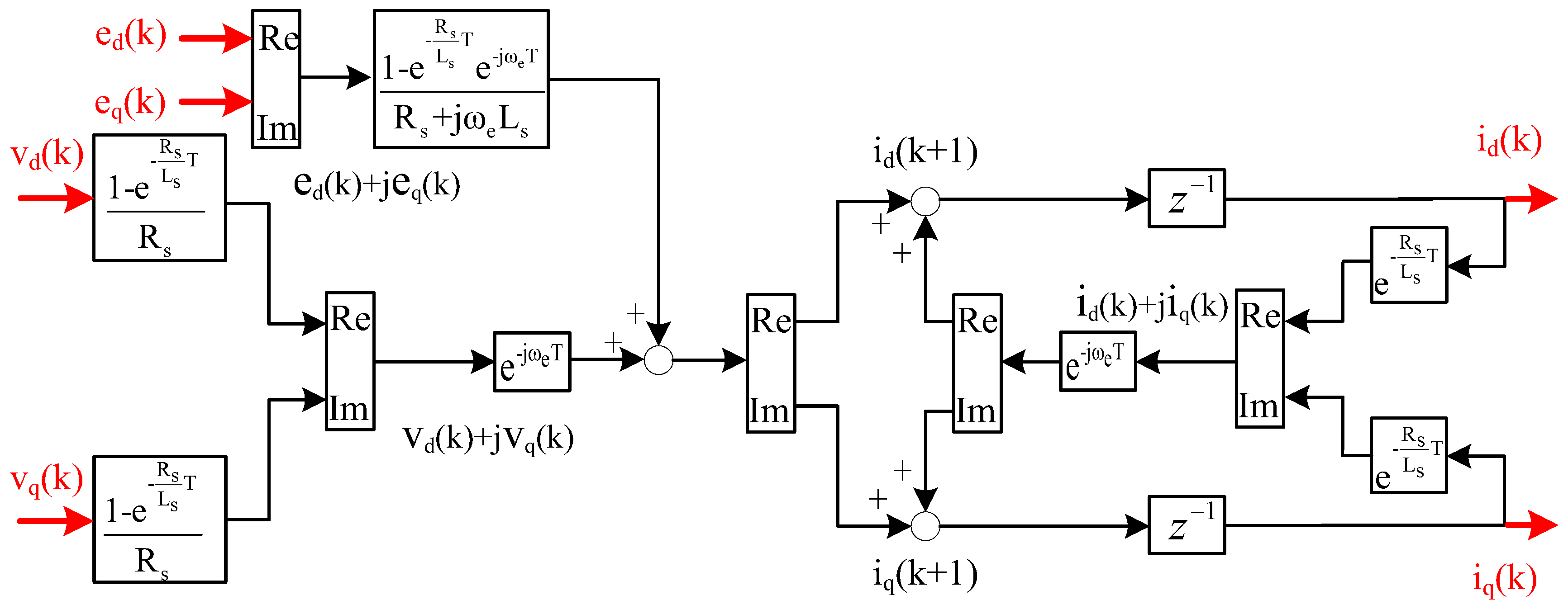
By substituting (6)–(8) into (4), the discrete-time machine model in the rotor frame is obtained by (9).
(9) shows the discrete-time machine model using the complex vector. The actual discrete-time response of both
(
kT) and
(
kT) can be demonstrated easily using the state space equation, which is given by
where the variables
F,
G,
EMF1 and
EMF2 are defined by (11)–(13) to simplify the equation in (10).
Figure 2 illustrates the corresponding discrete-time machine model with inputs of
(
kT), outputs of
(
kT) and disturbances of
(
kT)
. It is observed that a phase advanced term,
, appears in dq currents, voltages and EMF. According to the discrete-time model in (10), EMF voltages in the rotor frame can be directly calculated based on the relationship between
(
kT) and
(
kT) in
Figure 2 with the knowledge of
and
. It is shown to be:
In (14),
represents the estimated dq EMF voltages, and
is the estimated speed. In addition,
,
,
and
are calculated using the knowledge of
,
and
. In this paper,
and
are measured from a RLC meter offline. It can be noted that the open-loop EMF estimation in (14) is applied to obtain
. Because of open-loop estimation,
might be sensitive to the noises in
(
kT). However, for the high-speed operation, the magnitude of
is sufficiently higher than the resistance reflected voltage drop. In addition, as reported in [
30], the observer-based estimation might cause the phase lag in
due to the limited observer bandwidth at high speed. Considering this delay issue, the direct EMF calculation is implemented for the high-speed sensorless drive with low
.
It is important that the proposed discrete-time EMF estimation in (14) is substantially different to conventional continuous-time models in [
13,
14,
15,
16]. In particular,
is resultant due to the influence of ZOH, as seen in
Figure 2. As speed increases, the percentage of
on
increases, leading to additional estimation errors. Under this effect, the EMF estimation in (14) including the ZOH effect is suited for the sensorless drive at high speed.
Considering a perfect parameter estimation, the estimated dq EMF voltages
should be equal to actual EMF
(
kT), which is given by:
where
(
kT) and
are the actual rotor speed and magnet flux. It is important that in (15),
(
kT) should be zero, assuming the estimated position
is equal to the actual position
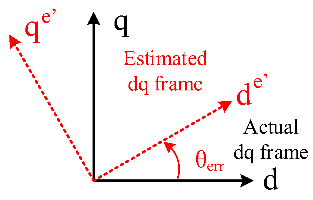
θe. For the sensorless drive at the initial state, the rotor position might be unknown before signal processing of the position estimation. Under this effect, there is a position error,
, between the estimated dq rotor frame and actual rotor frame, as seen in
Figure 3 where
(
kT)
= θe(
kT) −
(
kT). The subscripts,
e’ and
e, represent the estimated and actual rotor frame. Since the estimated
is initially located at the estimated frame,
should be modulated by sinusoidal functions dependent on the magnitude of
(
kT), which is shown to be:
For the purpose of the sensorless drive, the actual position can be obtained by manipulating (kT) to be zero. Detailed position estimation processing will be explained in the next section.
3. Position Estimation at High Speed
This section analyzes the position calculation using the spatial signal from estimated
. For the overall sensorless drive system, the corresponding signal process is implemented in the brown box of
Figure 1. On that basis, a PLL is developed to estimate the rotor speed
(
kT) and position
(
kT) with the position error,
(
kT) in estimated EMF. As seen in (16),
(
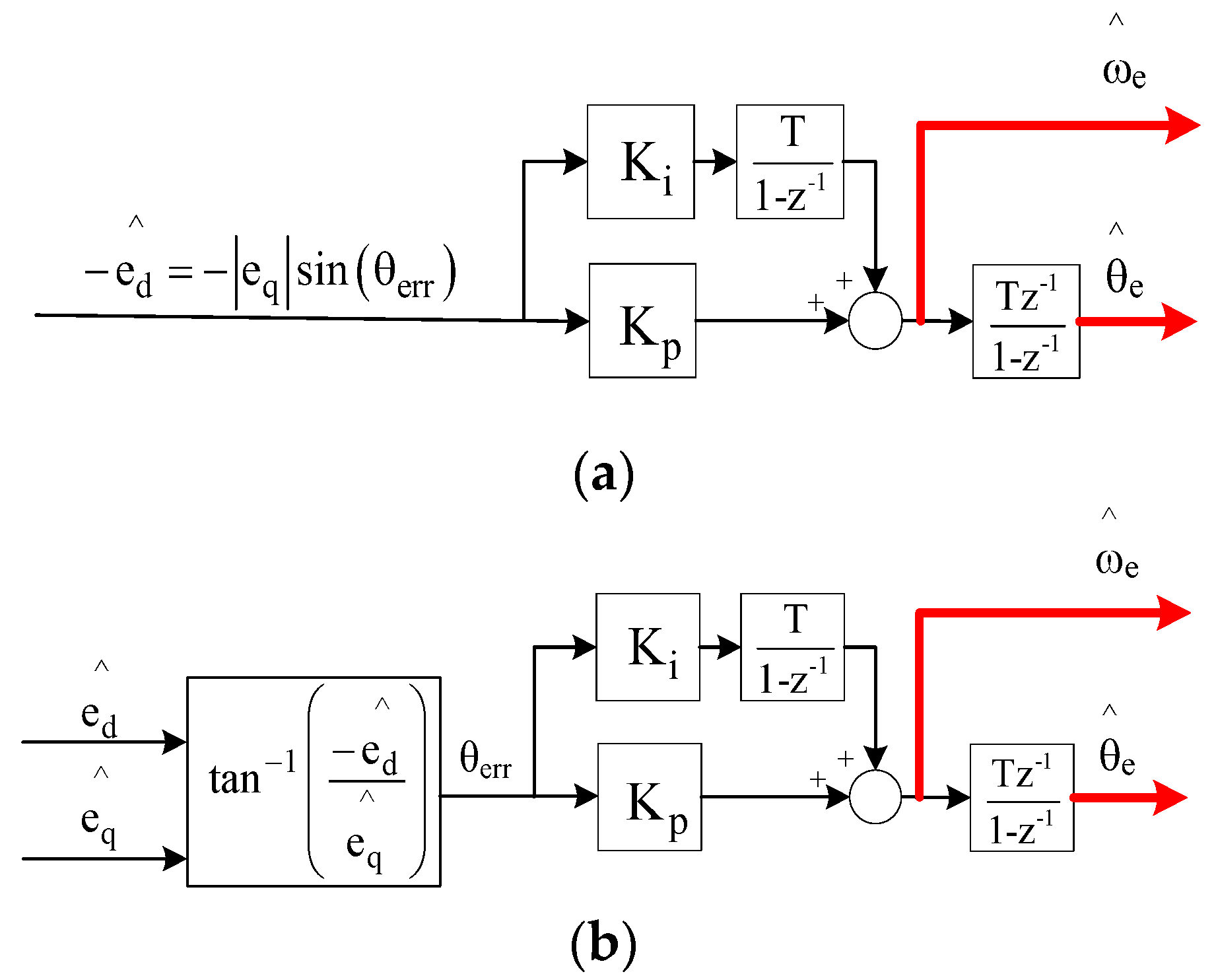
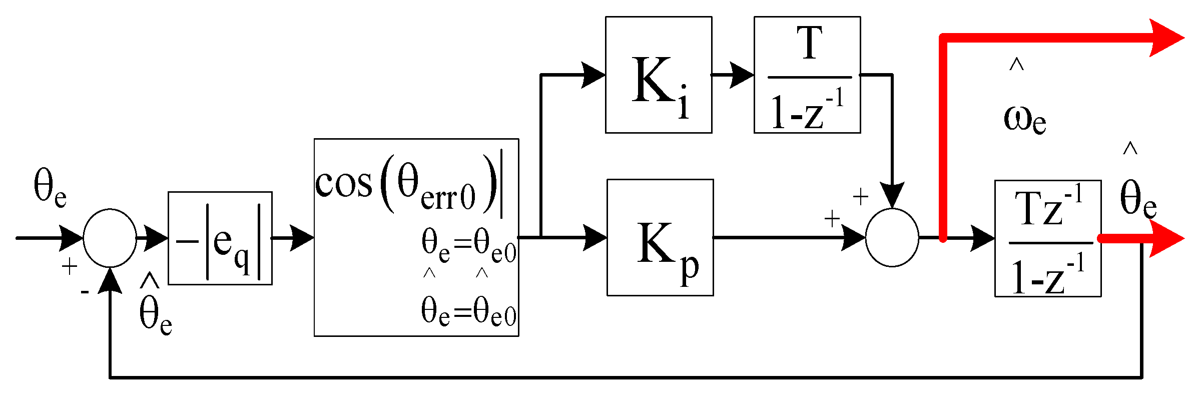
kT) can be extracted using either the small-signal approximation in (17) or the arctangent function in (18).
In (17), a small-signal approximation, where
(
kT)
= (
kT) −
(
kT), is assumed to simplify the nonlinear sinusoidal function in
. As illustrated in
Figure 4a, a PLL with a proportional gain
and an integral gain
is applied to estimate
(
kT) and
(
kT) by manipulating
to be zero. A backward approximation is implemented for the discrete-time integration in
Figure 4. In general,
determines the estimation bandwidth of PLL. If considerable harmonics are observed in
,
should decrease to reduce the error on
(
kT) and
(
kT). On the other hand, the steady state error might occur on
(
kT). This steady state estimation error can be removed by adding
. By properly assigning
and
simultaneously, the overall transfer function between
(
kT) and
can be formulated as a second-order low-pass filter to improve estimation performance.
On the other hand,
Figure 4b proposes a position estimation by adding an arctangent function in (18) cascaded to the same PLL. Due to the arctangent calculation, the small-signal approximation in (17) can be removed. At high speed, it will be demonstrated that the position estimation using the proposed PLL in
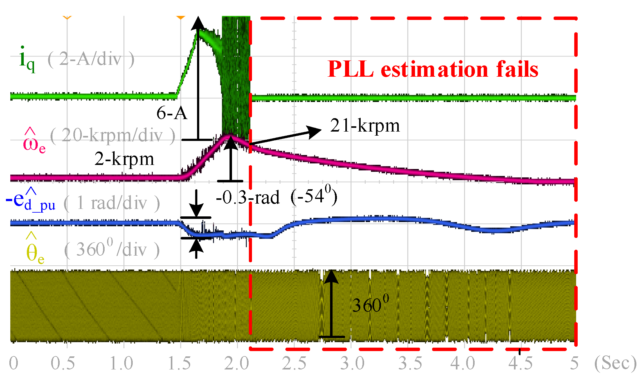
Figure 4b achieves better drive performance for the following three reasons.
3.1. Unit Length Feedback Signal
For the position estimation in
Figure 4a, the magnitude of
is proportional to
× (
kT), which is a speed-dependent signal. Under this effect, the speed-dependent estimation performance is resultant on
(
kT). As reported in [
38], the PLL might have a stability issue at low speed when
(
kT)
≈ 0 due to the low magnitude of
. Besides, at high speed the magnitude of
could be sufficient high. With the same
and
in
Figure 4, high-frequency noises in
might increase, leading to considerable position errors at high speed.
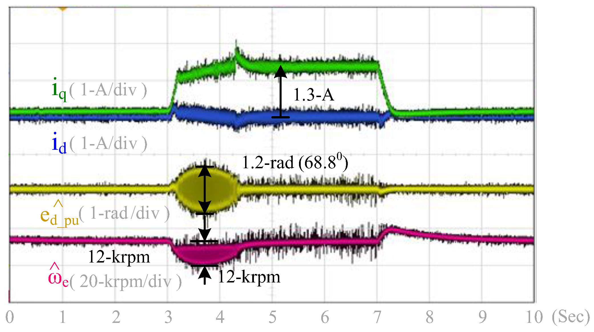
For the proposed estimation in
Figure 4b, a position error,
(
kT)
, with a unit length is extracted using the arctangent calculation. The speed-dependent term is removed, since both
and
contain the same value in any operating conditions. Compared to
Figure 4a, better position estimation performance based on
Figure 4b can be achieved.
3.2. Increased Dynamic Response
In addition to speed-dependent estimation bandwidth, the PLL structure in
Figure 4 also results in the discretized effect at high speed. Considering the low ratio of
, the assumption of
(
kT)
= (
kT) −
(
kT) ≈ 0 might not be valid for the positon estimation. For example, when
= 10-kHz,
= 1.67-kHz and
= 6, the position calculation period in the microcontroller is every 60° per electrical cycle. At this time, the resolution of sin[
(
kT)] is sin(60°) = 0.866, which might not be close to zero.
In order to analyze the accuracy of small-signal approximation in
Figure 4a, the nonlinear equation in (17) is linearized at two different operating points,
and
, to obtain an analytical model. On that basis, the partial derivatives of both
and
on sin(
−
) are applied, which are respectively shown to be
where
and
are the equivalent points with respect to
and
. According to (19) and (20), the nonlinear PLL in
Figure 4a can be linearized by
Figure 5 at different operating points,
and
.
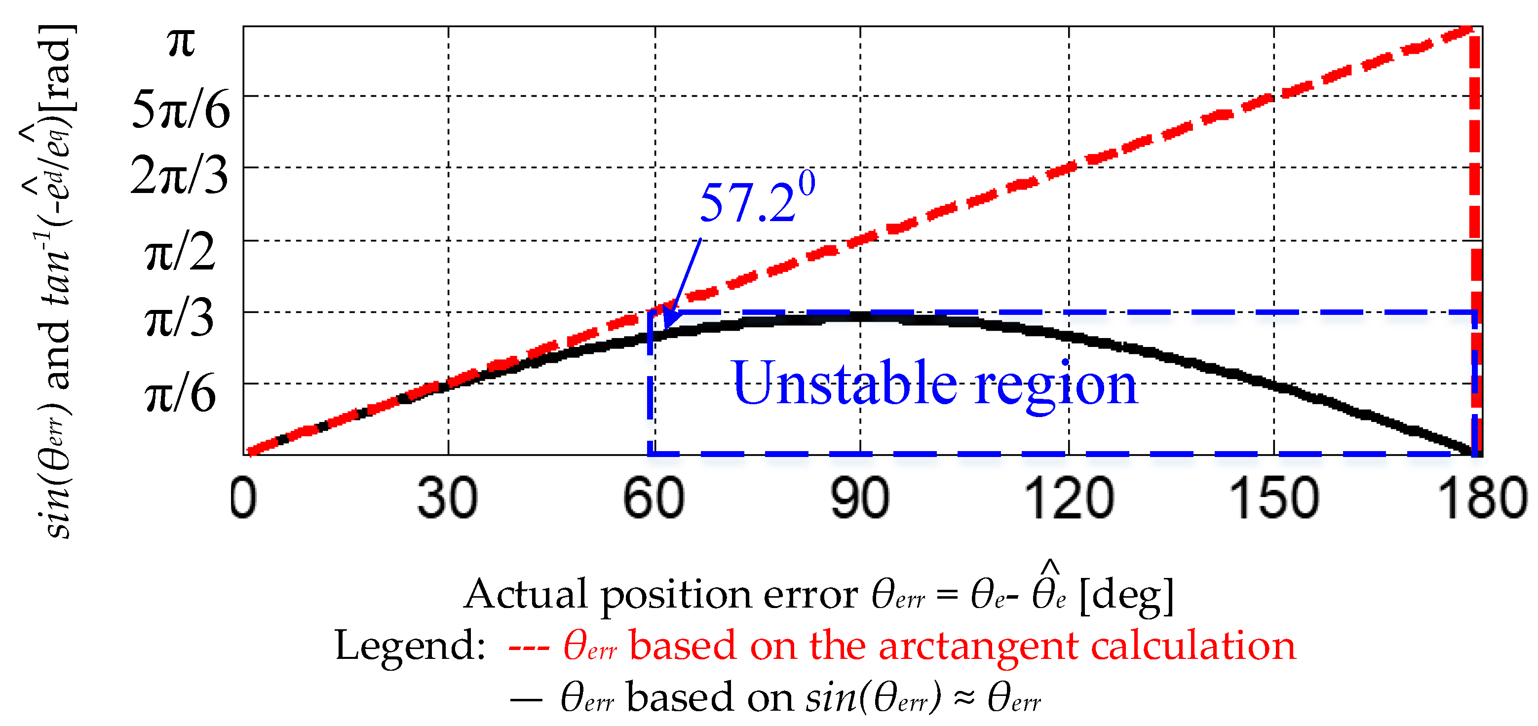
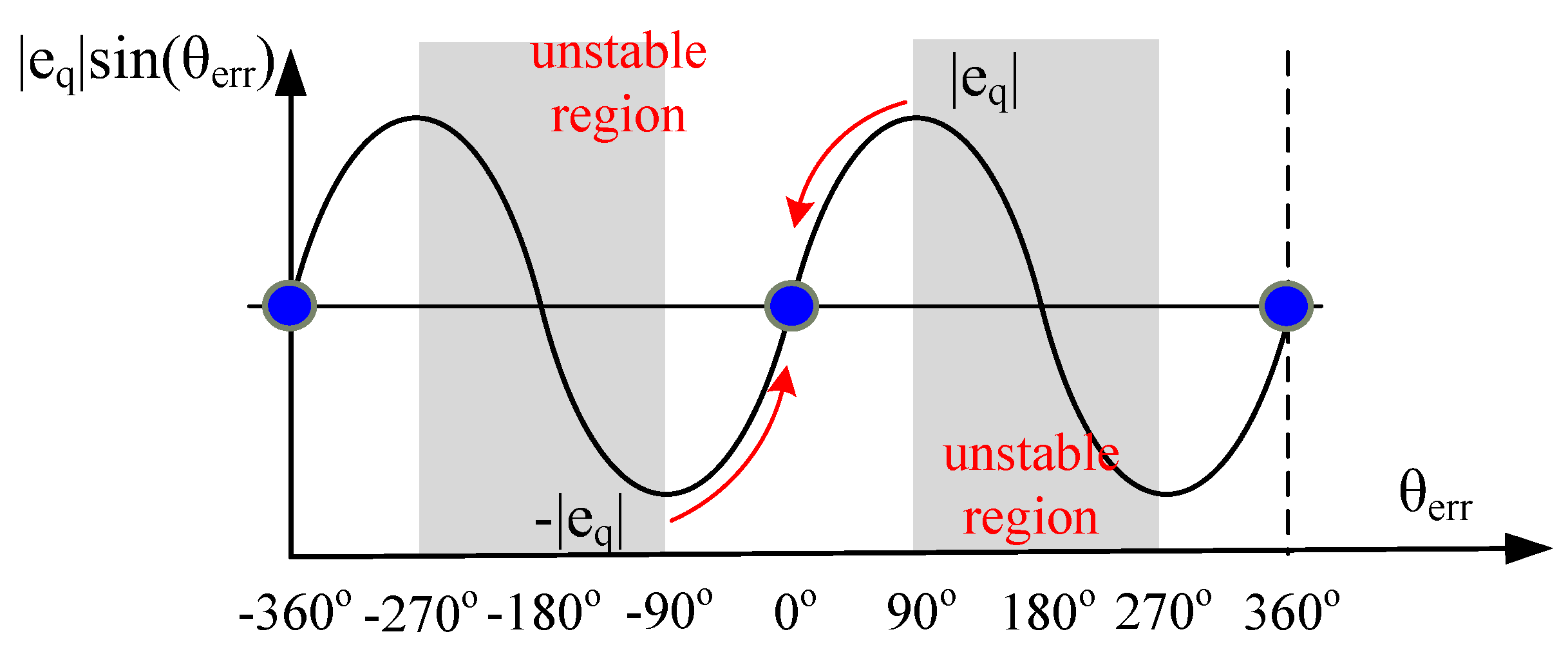
Figure 6 further compares the feedback spatial signals between
(
kT) from the arctangent calculation in (18) and sin[
(
kT)] based on the approximation in (17). The horizontal axis of actual
is used to analyze the error under these two different signal processes. Ideally, the value in the vertical axis should be equal to that in the horizontal axis as the actual
changes to the zero position error. It is shown that
(
kT) obtained in (18) increases linearly as actual
increases. The PLL estimation stability can be maintained up to actual
= 180°. On the other hand, sin[
(
kT)], based on (17), results in the unstable PLL estimation when actual
is beyond 90° due to the negative slope. More importantly, even in the stable region the deviation between sin[
(
kT)] and
(
kT) significantly increases when actual
reaches 60°. Considering the dynamic operation at high speed,
(
kT)
= (
kT) −
(
kT) cannot be maintained at zero during the speed and load transient. Degraded drive performance must result, due to the approximation error shown in
Figure 6.
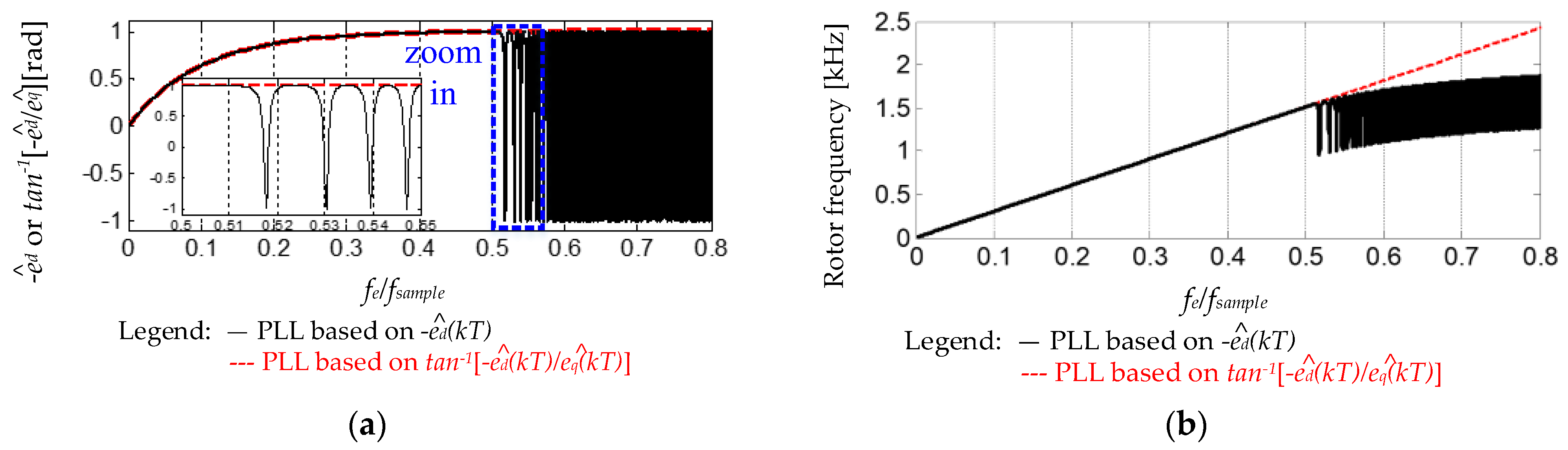
Figure 7 shows the simulation results of (a) feedback spatial signals, the normalized
and
and (b) the estimated rotor frequency
versus time. In this simulation, the speed-dependent component |
eq| in
of (17) is removed to obtain the normalized
in order to easily compare the result using
The rotor frequency
is controlled to increase from 0–2.5 kHz (
decreases from ∞ to 4). The acceleration rate is 3 kHz/s to analyze the limitation in (16) under the dynamic operation. In this case,
and
in (a) all contain a certain amount of error due to the rapid acceleration. However, when
is close to 1.5 kHz, the feedback signal,
= sin[
(
kT)], reaches 1, leading to the positive feedback in PLL, as illustrated in
Figure 8. A considerable oscillation on
is then induced, where
varies between −1 and 1. Based on this simulation, the PLL estimation in
Figure 4a loses the stability when
≥ 1. On the contrary, due to the linear relationship between
and actual
, the PLL in
Figure 4b performs well under this rapid acceleration.
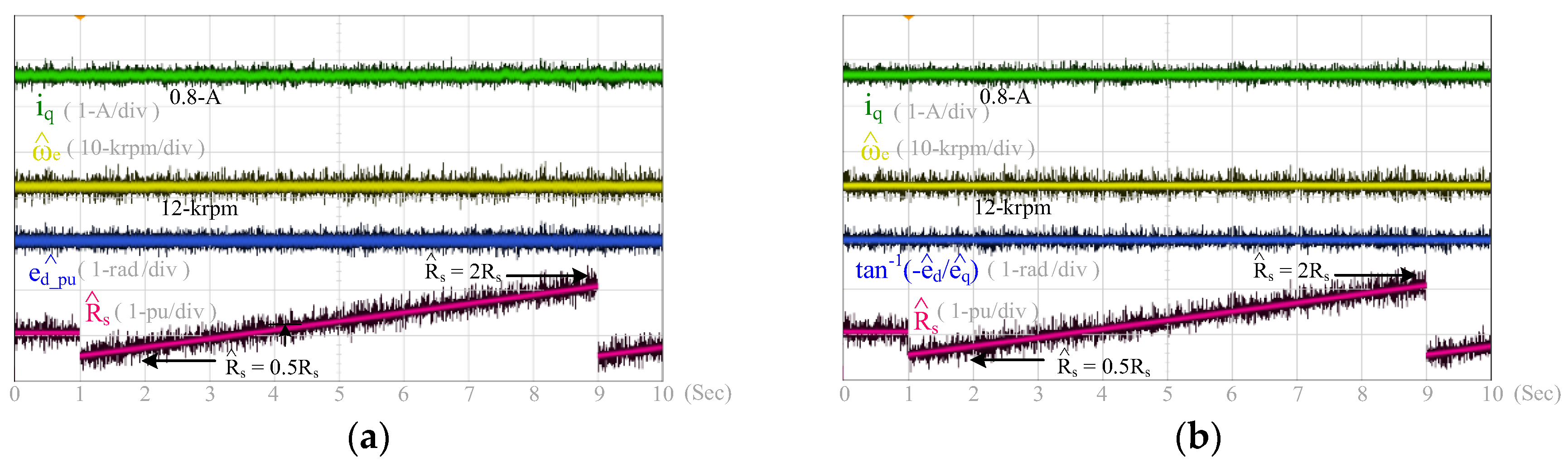
3.3. Reduced Sensitivity on the Parameter Error
In addition to the improved dynamic operation, the PLL estimation in
Figure 4b also achieves reduced sensitivity on the machine parameter variation compared to the estimation in
Figure 4a. Considering the parameter error, the EMF estimation in (14) should be modified by
where
are estimated EMF voltages with the parameter error, and
and
are additional components due to estimation errors from the resistance and inductance. Assuming the resistance and inductance estimation error are Δ
=
−
and Δ
= −
,
and
can be obtained from (14), which are shown in (22) and (23), respectively.
where
It is noteworthy that both (22) and (23) contain the
dependent term. Thus, Δ
and Δ
all cause speed-dependent errors in estimated
and
under the digital implementation.
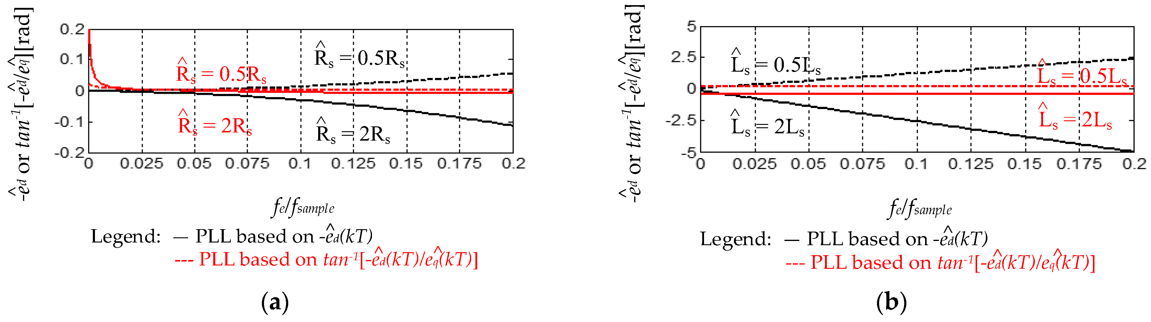
Figure 9 analyzes feedback signals of
and
versus
, considering the parameter estimation error. In this simulation,
and
(
kT) in (21) are calculated by adding
and
. As shown in (a), the error of Δ
results in
dependent error on
, where the error increases as
increases. For the PLL estimation in
Figure 4a, an increased error on
at high speed should appear, leading to the reduced torque output. By contrast, the PLL in
Figure 4b based on
is immune to Δ
once
is higher than 0.025. By obtaining
(
kT) in (18), the position estimation performance can be insensitive to Δ
at high speed.
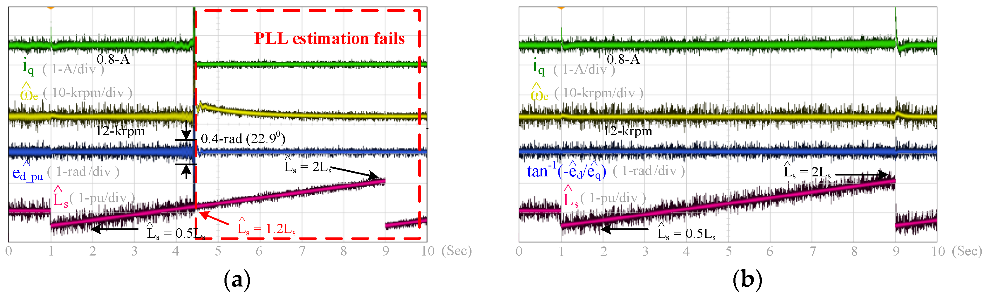
For the inductance variation in
Figure 9b,
dependent error also appears in
More importantly, the error on
due to Δ
is significantly higher than that due to Δ
at high speed. Considering the inductance leakage effect and saturation at high speed, PLL estimation using only
can lead to a stability problem. On the contrary, a constant error on
is observed. The use of both d- and q-axis EMF voltages for the position estimation is the key for reducing the inductance variation at high speed with low
. Based on this simulation, it is concluded that the reduced parameter sensitivity on the sensorless drive can be achieved using the proposed PLL estimation in
Figure 4b.
Table 1 lists the performance comparison between the PLL estimation in
Figure 4a,b. Two advantages on the proposed PLL in (b) are summarized:
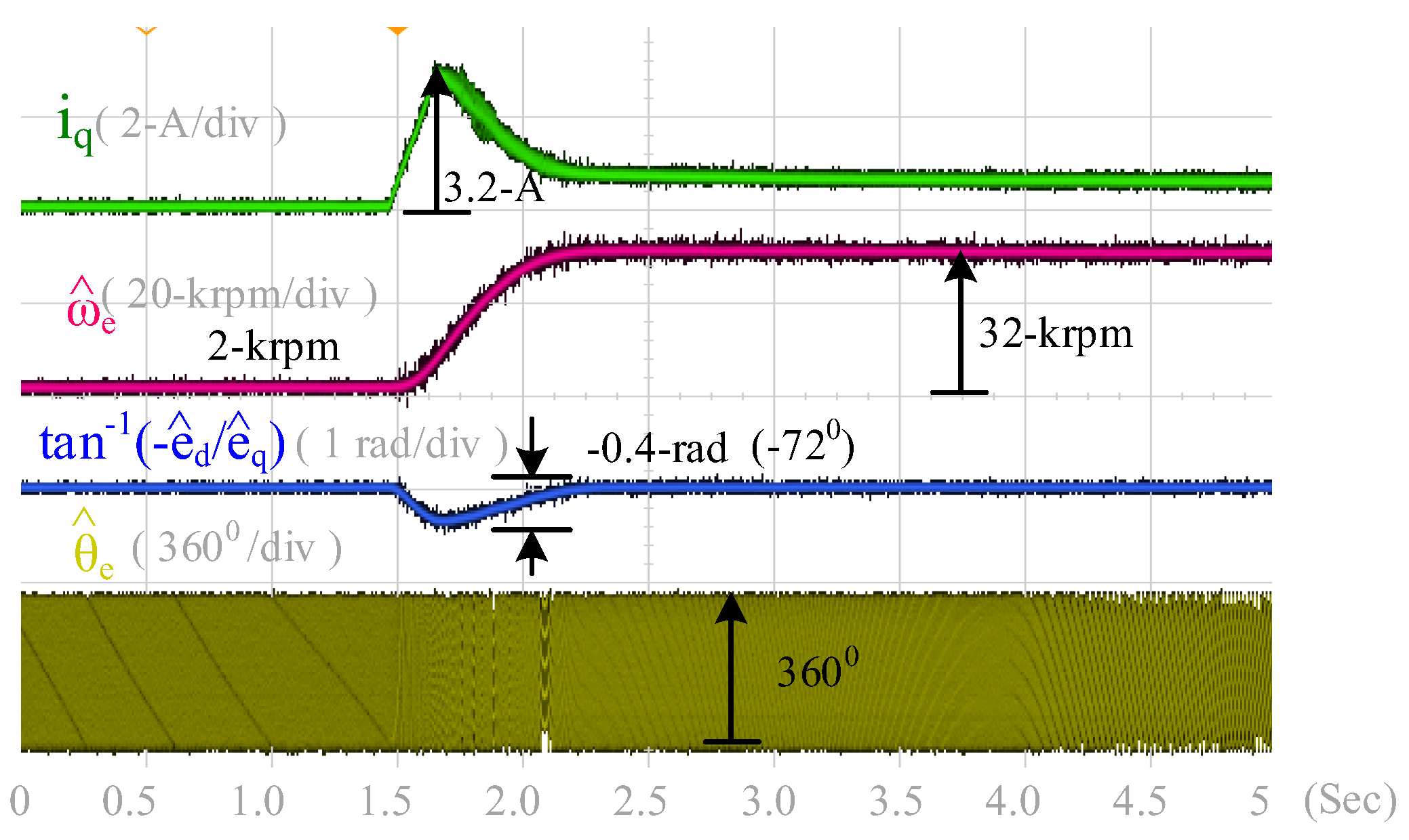
The dynamic response is improved at high speed. As seen for the feedback position error signal in
Figure 7, the nonlinearity of sin(
) appears once the position error between the estimated and actual position is higher than 57.2°. After adding the arctangent calculation, the signal of tan
−1(
/
) still maintains a linear waveform once the position error reaches 180°. Thus, a better estimation performance is achieved.
The PLL cascaded the arctangent calculation also shows reduced sensitivity on the parameter variation at high speed. As seen in
Figure 9, tan
−1(
/) receives the position information from both
and
. Compared to the conventional PLL obtaining the position information from only
, it can be concluded that there is reduced sensitivity on the parameter. In addition, due to the reduced parameter sensitivity, the overall drive stability can also be improved using the proposed PLL.


