Two-Stage Electricity Demand Modeling Using Machine Learning Algorithms


Department of Informatics, Faculty of Applied Informatics and Mathematics, Warsaw University of Life Sciences, Nowoursynowska 159, 02-787 Warsaw, Poland
*
Author to whom correspondence should be addressed.
Energies 2017, 10(10), 1547; https://doi.org/10.3390/en10101547
Submission received: 21 August 2017
/
Revised: 28 September 2017
/
Accepted: 2 October 2017
/
Published: 8 October 2017
(This article belongs to the Special Issue From Smart Metering to Demand Side Management)
Abstract
:Forecasting of electricity demand has become one of the most important areas of research in the electric power industry, as it is a critical component of cost-efficient power system management and planning. In this context, accurate and robust load forecasting is supposed to play a key role in reducing generation costs, and deals with the reliability of the power system. However, due to demand peaks in the power system, forecasts are inaccurate and prone to high numbers of errors. In this paper, our contributions comprise a proposed data-mining scheme for demand modeling through peak detection, as well as the use of this information to feed the forecasting system. For this purpose, we have taken a different approach from that of time series forecasting, representing it as a two-stage pattern recognition problem. We have developed a peak classification model followed by a forecasting model to estimate an aggregated demand volume. We have utilized a set of machine learning algorithms to benefit from both accurate detection of the peaks and precise forecasts, as applied to the Polish power system. The key finding is that the algorithms can detect 96.3% of electricity peaks (load value equal to or above the 99th percentile of the load distribution) and deliver accurate forecasts, with mean absolute percentage error (MAPE) of 3.10% and resistant mean absolute percentage error (r-MAPE) of 2.70% for the 24 h forecasting horizon.
1. Introduction
Short-term load demand forecasting up to 24 h in advance is essential for the efficient and secure management of power systems. Load forecasting is concerned with different horizon scales: hourly, daily, weekly, monthly, and annual values for both overall demand and peak demand. Importantly, short-term forecasting has attracted a great deal of attention in the literature due to its applicability in power system management, including resource planning and taking control actions towards load balancing [1,2,3]. Other forecasting horizons, for example in the medium- and long-term, are necessary for system planning, investment, and budget allocation. Imprecise load forecasting may cause an increase in terms of the operating cost of the network [4,5]. In particular, overestimation of the demand results in excess supply, and it may be problematic in balancing the network, while underestimation of the load may lead to a failure in delivering enough reserve, which entails the high costs of producing extra load units.
Delivering an accurate and robust load forecasting methodology requires tools with strong nonlinear mapping capabilities since demand data often present nonlinear patterns. Moreover, socio-behavioral, economic, and environmental factors may influence electricity consumption. This results in hourly, daily, weekly, and seasonal fluctuations in electricity consumption patterns and the existence of peak periods characterized by abnormally high consumption levels [6,7,8].
In this paper, we investigate a two-stage approach to forecast the hourly electricity loads in the overall national power system 24 h ahead by taking into account predictions from demand peak classification models. The models are trained to identify an extraordinary load level, equal to or above the 99th, 95th, or 90th percentiles for respective load distribution when considering the loads of weekly time windows. The scores from classification models then feed the forecasting models. Thus, more accurate short-term forecasts can be proposed as compared to the basic model without additional, peak-related features.
Specifically, based on simulation experiments we aim to find the answers to the following research questions:
- (1)
- Is it possible to deliver accurate demand peak load classification for a forecasting horizon 24 h in advance?
- (2)
- Is it possible to deliver accurate load demand forecasting 24 h ahead? To what extent?
- (3)
- Do the additional variables related to the predicted peak loads improve demand forecasting 24 h ahead?
- (4)
- What algorithms are appropriate for the two-stage modeling approach in order to deal with this kind of hourly data?
The reminder of the paper is structured as follows: a literature review on related problems is provided in Section 2. The data characteristics and their mapping into the binary classification problem (peak identification) and the load forecasting in the Polish power system [9] are presented in Section 3. Then, in Section 4, a comprehensive description of the proposed two-stage modeling approach is presented. The empirical analysis and comparison of the algorithms are used for both classification and forecasting problems, and the summary of the results are presented in Section 5. Finally, Section 6 concludes the paper and outlines direction for future research.
2. Literature Review on Related Problems
Electricity demand management applies to effective utilization of the available energy resources, system reliability, energy conservation, and other actions that promote energy efficiency for sustainable development. Managing limited energy resources in an optimal way has become a primary goal among energy suppliers, energy planners, policy makers, and governments. In this context, demand management is supposed to deliver self-sufficiency and cost-effectiveness leading to solid and sustainable economic development. In particular, the motivation of the research stream in this area is focused on, inter alia, demand forecasting, electricity price forecasting, identification of conservation needs, identification of new energy resources, optimized energy utilization, methods for energy efficiency intensification, and strategies for reduced emission of gases.
A considerable amount of research has been dedicated to electricity price forecasting. As investigated by Weron [10], there were more than 800 publications related to electricity price forecasting in the years 1989–2013, as indexed in the Web of Science and Scopus databases. While there is a high saturation of scientific articles, there are only three books that address electricity price forecasting, which are those of Shahidehpour et al. [11], Weron [12], and Zareipour [13].
Energy forecasting models can be systematized in several ways, categorized as static or dynamic, univariate or multivariate, or as involving various techniques ranging from simple naive methods through a wide range of times series methods to complex hybrid and artificial intelligence models. A wide variety of forecasting approaches has been proposed in the literature, and these fall into several research streams. For the purpose of the review, the approaches are categorized under the following headings: (1) statistical and time series models; (2) computational intelligence models; and (3) hybrid models.
Under the first category of statistical and time series models are a number of approaches which are the applications of statistical or econometric methods including regression models, macro-economic econometric models, cointegration models, autoregressive integrated moving average (ARIMA)-type models, decomposition models, and gray prediction models.
Time series models are the most frequently used methods to represent the future values based on previous observations. The models based on time series have many forms adequate for forecasting electricity consumption volume and peak demand load in the electrical grid. These models are often applied to demand forecasting at the regional/national level. For instance, Himanshu and Lester [14] used six different time series approaches for predicting electricity demand in Sri Lanka and the forecasts from these techniques look fairly similar considering the horizon of the year 2025. Others, like Gonzalez-Romera et al. [15] applied an approach to monthly energy forecasting for Spain, in which two time series are considered separately: the trend, and the fluctuation around it.
Regression models are built to capture a relationship between a dependent variable, which is the energy usage, and one or more independent variables (the predictors). These models were used by Jannuzzi and Schipper [16] to analyze the electrical energy consumption of the residential sector in Brazil. An interesting finding was that the electricity demand increased faster than the income. In [17], linear and nonlinear effects between energy consumption and economic growth in Taiwan were explored by Lee and Chang, based on data over the period 1955–2013. In [18], a linear regression model was used by Yumurtaci and Asmaz to predict electricity consumption in Turkey based on the population size and energy consumption increase rates per capita.
Econometric models are built to investigate dependencies between the energy demand and other macro-economic variables such as energy price, gross national product (GNP), technology, investments, and population size. For instance, Samouilidis and Mitropoulos [19] studied energy and economic growth over the 1960s and the 1970s in industrialized countries, suggesting decreasing income and energy price elasticity. Others, such as Sengupta [20], have demonstrated that econometric models are effective for forecasting energy patterns in developing countries like India. Quite often the econometric models are proposed to forecast demand for different electricity sources, e.g., coal, oil, and different sectors including industry, transportation, and residential end users in industrialized [21] and developing [22] countries.
Among a wide range of econometric methodologies used to capture energy demand relationships, cointegration models were found to change the perception of researchers and practitioners towards electricity demand forecasting [23]. According to the cointegration concept, non-stationarity of the variables indicates that there is no long-run (cointegrating) relationship between them, and the regression results may be spurious, as concluded by Hasanov et al. [24]. This indicates that only stationary variables should be considered in the analysis, and, as an alternative, if cointegration is observed amongst non-stationary variables, then the regression results suggest long-run relationships as being present in data.
There are two common approaches to build decomposition models for which energy consumption (EC) and the energy intensity (EI) analysis can be distinguished. The terms EC and EI indicate the energy-related variable subject to decomposition. As explained in [1], these effects are “associated with the change in aggregate production level, structural change in production, and changes in sectoral energy intensities, while in the energy intensity approach only the last two effects are considered.” For instance, the relevant application issues, including method selection, period-wise against time-series decomposition, and the importance of sectorial disaggregation were analyzed and thoroughly reviewed by Ang [25].
The ARIMA models describe the approximate model of data sequences over time, assuming the lag term and random error term to explain and to predict the future outcome with a certain mathematical formula [26]. Univariate Box–Jenkins autoregressive integrated moving average (ARIMA) analysis has been widely applied to forecasting in many fields, including environmental, medical, business and finance, and engineering problems [1,26,27].
Gray models for prediction gained popularity due to their simplicity and ability to describe unknown relations, even when using only a few data points. As argued by Chiang et al. [28] energy demand forecasting can be considered as a gray system problem, because only a few variables such as GDP, investment, and population size are known to contribute to the energy demand, but the exact relations and the method of affecting the energy demand is not necessary clear or even unknown. The family of gray forecasting models consists of several types and GM(1, 1) is commonly used for forecasting energy demand, as presented by Hsu and Chen [29].
Within the category of computational intelligence methods, we can distinguish a number of artificial intelligence-based, neural network, support vector machine, non-parametric, and non-linear techniques, which combine elements of learning, evolution, and fuzziness to create robust approaches that are capable of modeling complex and dynamic systems.
Over the last two decades, a great research stream has been dedicated to the application of artificial neural networks (ANNs) and expert systems for electricity load forecasting. ANNs, with their high modeling capability and their ability to generalize non-linear relations, gained widespread popularity for general forecasting in a variety of business, industry, and science applications [30,31]. Neural network models have been extensively studied and successfully applied to short-term electricity forecasting [32,33,34,35]. Some researchers have worked on ANN models applicable to medium- and long-term forecasting [36,37]. Cincotti et al. [38] proposed two computational intelligence techniques, ANN and the support vector machine, to model electricity spot prices of the Italian Power Exchange. The results indicate that support vectors give better forecasting accuracy, closely followed by the econometric models.
Recently, within the smart metering and smart grid initiatives, there has been increasing interest in residential power load forecasting. For this purpose, a number of neural networks and expert systems are applied to load forecasting at the individual household level [39,40,41]. However, this is a challenging task due to the extreme system volatility, which is the result of different dynamic processes composed of the typical, mostly behavioral and socio-demographic, components of many households. Aggregation of individual components reduces the inherent variability of electricity consumption resulting in smoother load shapes; as a result, the forecasting errors observed at the higher aggregation levels (power stations or regions) have been quite low.
Over the last couple years soft computing techniques including genetic algorithms and neuro-fuzzy and fuzzy logic models have been more frequently applied in energy demand forecasting. For instance, Tzafestas and Tzafestas [42] analyzed eight case studies to show the merits, and validate the performance, of the various computational intelligence techniques constructed under a large repertory of data including geographic and weather features. Ozturk et al. [43] applied genetic algorithms for forecasting the electricity demand in Turkey. The models were successfully validated with actual data, while future estimation of electricity demand was projected up to 2025. Ying and Pan [44] proposed an adaptive network based on the fuzzy inference system to forecast electricity loads in four regions of Taiwan.
Based on the available literature, there is a clear and increasingly recognizable research interest that looks at the application of various hybrid models, combining techniques from two or more of the groups listed above. This stream is aimed at increasing the load forecasting accuracy by benefiting from the best features associated with different approaches and their synergy. For instance, in [45], the authors combined the ARIMA forecasting model, the seasonal exponential smoothing model, and the weighted support vector machines for short-term load forecasting. They demonstrated that the combined solution can effectively account for the nonlinearity and seasonality to benefit from more accurate forecasting results. In [46], Pao proposed two hybrid nonlinear models as a combination of a linear model with an ANN to create an adjusted forecast. The superiority of the hybrid is due to their flexibility in accounting for complex hidden relationships that are difficult to capture by linear models.
In [47], Amjady and Kenya proposed a hybrid method composed of cascaded forecasters where each block consists of an ANN and an evolutionary algorithm. Such a structure was able to deliver high effectiveness and outperformed a combination of similar day and ANN techniques.
Within the research stream dedicated to load forecasting, there is considerable interest in electrical peak load forecasting. Peaks may cause serious challenges to the electricity grid because it needs to support the abnormally high consumption load. Managing these peaks is crucial for the utility providers since energy deficiency can lead to severe consequences such as power outages. Electricity consumption peaks appear in the electricity system as a consequence of the joint behavior of end users, which is influenced by many external factors [6,7,48]. An example of an aggregate behavior is when a relatively large group of individual consumers turns on air conditioners within a short time span because of high temperatures. This behavior is easy to notice since temperature increase affects a large population, which might cause the peak. However, there are other factors that are likely to influence users’ electrical consumption; therefore, it is not trivial to detect high loads in advance. Luckily, peak loads usually follow similar patterns [49,50], and these can be identified with, inter alia, classification and pattern recognition algorithms to be further used to improve the accuracy of the forecasts, as presented in our paper. For instance, in [6], the authors proposed the approach to predict electricity consumption peaks as an input to load balancing and price incentive strategies. This was done by mapping the prediction activities into a two-labeled classification problem. The authors declared that the solution was able to detect about 80% of consumption peaks considering a forecasting horizon of up to one week. A different approach was chosen in [7] to find some characteristic patterns in data that may determine changes in the demand peaks. Then, the classification of the load curves into groups was proposed to give the analytical space for couple of functional linear models used to make peak load forecasts. Another interesting proposal was presented by Hyndman and Fan in [48] as an application to forecast probability distributions, including 10%, 50%, and 90%, of weekly and annual peak electricity demand up to 10 years ahead for South Australia.
Based on the literature review, research on electricity load forecasting is maturing, with numerous approaches and attempts proposed throughout the last several decades. However, there is still an increasing and recognizable need to look at the challenges associated with behavioral factors that influence the energy usage considered at different aggregations, including individual end users, micro-grids, and region or country levels. Since peak load forecasting plays an important role in the effective management of power utilities, it falls under one of the current research streams focused on predicting the peaks as an input into load balancing and smart management strategies. These are intended to achieve, in the future, automatic behavior at the customer end, including automatic management of smart electrical appliances (controlled switch on–off events), supporting local level load balancing.
With this paper, it is expected that the proposed two-stage modeling approach will help energy planners to forecast more accurately and to utilize energy resources in a sustainable way by reducing the cost of operating power systems.
3. Dataset Characteristics
3.1. Load Data
This study was performed based on historical data representing energy consumption in the Polish power system [9]. The data set included 70,128 observations of hourly data covering the time window between 1 January 2008 and 31 December 2015. As shown in Figure 1, a time series of the Polish power system exhibited annual, weekly, and daily seasonal cycles.
The daily load curves have different shapes depending on the day type (workday, Saturday, Sunday, or holiday) and the season. Figure 2 presents a smooth profile shape with relatively low electricity usage at night and in the early morning, clearly defined peaks in the evenings, and slightly smaller defined peaks in the late morning. Electricity usage is significantly lower during the weekend or holiday days. On Wednesday (11 November), there was a national holiday, which resulted in low electricity demand.
Fluctuations in the daily load characteristics and the load volume during the seasons of the year are influenced by weather conditions including temperature, humidity, wind, cloud coverage, and precipitation, as well as day length. When it comes to weekly cycles, these are determined by workdays, weekend days, and holidays. These multiple seasonal cycles in the electricity consumption along with the trend and non-stationarity in mean and variance have to be reflected in the forecasting algorithm in order to build a robust and an accurate solution.
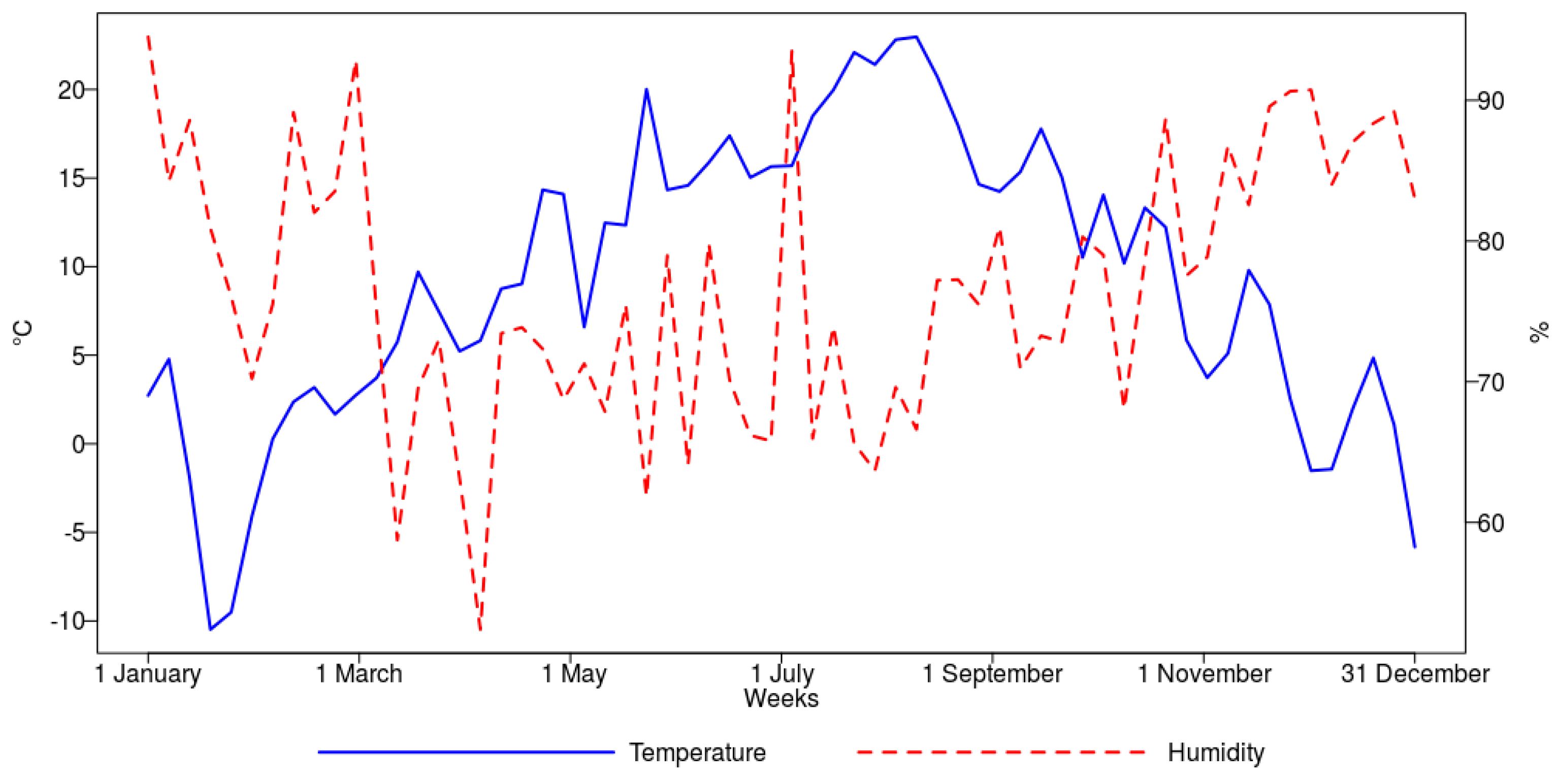
3.2. Weather Data
Weather is one of the most important independent variables for electricity forecasting. Temperature and humidity are features that are often used in the forecasting models to describe weather conditions. An example of weekly average temperature and humidity data in Warsaw in 2015 is presented in Figure 3. Unexpected weather conditions are often considered as the tipping point that can cause a severe instability of the system and decrease its efficiency in terms of the power supply. For instance, unexpected thunderstorms in the middle of sunny day are one of the environmental factors that can suddenly decrease the temperature and thus lead to an overestimated load prognosis [51], resulting in production of more power than is actually required.
As argued by Fahad and Arbab [52], there is a high and positive correlation between the temperature and the load volume during the summer season, while there is a negative correlation between the temperature and the load volume during the winter. In other words, in the summer, a certain temperature increase will result in a load increase, and going forward a temperature decrease will result in a decrease in the average daily load and a lowering of the peak volume. In the winter, an opposite trend is observed, as a decrease in the temperature will result in an increasing demand for electric load. Such regularity is because in the summer an increase in temperature affects consumers who use electricity for cooling purposes (air conditioners and fans), whereas in the winter electricity is predominantly used for heating homes.
Another weather factor influencing overall load curve is humidity. In practice, it is referred to as relative humidity, and it is expressed using percentage values. There is a common observation that humidity can affect apparent temperature perceived by individuals, while it has no effect on the real temperature. However, humidity can make a 33 °C temperature seem more severe, say 40 °C.
3.3. Determining Peak Values
In order to determine peak load values, the generic function quantile implemented in R was used [53]. The function produces sample quantiles corresponding to the given probabilities by the weighted averaging of order statistics Zg:
where γ = np + m − g, n is the number of observations, g = floor(np + m), and m = 1 − p.
Qp = (1 − γ)Zg + γZg + 1
In this study, peak load was determined as the load value equal to or above the 99th, 95th, or 90th percentile for a given load distribution when load was grouped for each week, as presented in Figure 4.
In the figure, the black curve shows the hourly electricity consumption observed in November 2015. The blue line reflects the average load within a particular week, and the red line shows the threshold values above which the loads are recognized as peak values. Finally, the green dots stand for the peak load exceeding the 90th percentile of the distribution.
4. Two-Stage Modeling Approach
4.1. General Idea of the Approach
The idea of the approach is to forecast short-term electricity loads by taking into account predictions from demand peak classification models. The models are trained to identify the extraordinary load levels, which are equal to or above the 99th, 95th, or 90th percentile for the respective load distribution when the weekly time windows are considered. The scores from the classification models are used to enhance the forecasting models; thus, more accurate short-term forecasting can be proposed as compared to the basic model without additional, peak-related features.
The proposed predictive solution consists of two main phases, namely the peak classification phase and the forecasting phase (see Figure 5, which presents the graphical illustration of the approach).
4.1.1. Data Processing
The inputs of the proposed system are the weather data and data, reflecting the load of the Polish power system. From these time series, a set of 97 independent variables was extracted (see Section 4.2 for variables details). All the missing values were imputed using a moving average over a sliding window of 5 h.
4.1.2. Peak Classification Phase
The classification phase consists of two stages. Within the first stage, only the independent variables that had the best discriminatory power were determined (see Section 4.3 for more details). Next, based on the derived variables, three classification models were built to identify the load levels that are equal to or above the 99th, 95th, or 90th percentile of the distribution. The models were focused on electrical power consumption peak detection in the power system based on historical data for both electricity usage and the weather conditions data, including temperature and humidity. In this way, we deal with peak detection as a binary classification problem, unlike most previous studies where the problem is formulated as time series forecasting.
4.1.3. Additional Features
In this stage, three additional features based on the classification models are constructed. These additional features are the classification scores, indicating the probability that peak load will occur. In order to benefit from the optimal score threshold, which determines the peak (score above the threshold) or normal load (score below the threshold), Youden’s J statistic [54] was applied. The optimal cut-off is the value that maximizes the distance to the identity (diagonal) line. The optimality criterion is defined as:
where Tpr is the proportion of positives (peaks) that are identified correctly. As such, Fpr is the ratio of negative events (non-peaks) wrongly classified as positive (false positives) to the total number of actual negative events.
max(Tpr + (1 − Fpr))
4.1.4. Forecasting Phase
In this phase, we will study an approach to forecast the hourly electricity demand of the Polish power system for the 24 h ahead, taking into account the same feature vector as in the case of the classification models (see Section 4.3 for details) to produce a basic forecasting model. Enhanced forecasting models will be built on the extended feature vector, including variables that come from the peak classification models for the different quantiles, i.e., the 99th, 95th, or 90th quantiles.
4.1.5. Evaluation
To evaluate the models, the data were split into the training, validation, and test datasets. After the two-stage modeling approach, the predicted values from these datasets were compared with the true electricity consumption values. A set of commonly used and acknowledged performance measures was calculated to evaluate the quality of the forecasts.
4.1.6. Improved Forecast
Finally, the two-stage modeling approach is to enhance the short-term forecasting of Polish power system loads. The outcome of this stage is to present improved forecasts able to detect underlying dependencies in analyzed data.
4.2. Feature Vector
We focused on the next-day peak power demand classification and electricity load forecasting. For both exercises, a feature vector with the attributes as listed in Table 1 was constructed. The attributes were derived from historical time series data recorded at hourly intervals. Additionally, external features were collected, including weather condition data represented by the sunset information, the temperature, and the humidity. Calendar variables were considered as well.
The main variables taken into account for the modeling are these extracted directly from the load curve (Attributes 1–78 as presented in Table 1). The features were prepared by time series decomposition, and they define, among other characteristics, linear trend, actual hourly demand, and average demand at certain intervals, taking into account information up to 7 days prior.
Electricity demand fluctuates over time and types of cycles. Fluctuations in daily, weekly, monthly, and seasonal demand, as well as those related to holidays can be observed in the data. Therefore, the analysis was enriched with an additional 19 variables, including 5 variables describing the hour, 5 variables representing the day of the month, 3 variables used to decode the day of the week, 4 variables associated with the month, 1 holiday indicator variable, and 1 variable indicating the hour of the sunset. All the above time and calendar variables were derived in the following manner (bit encoding instead of standard dummy encoding): firstly, all the categories were presented as ordinal, these integers were then transformed into binary code, and the digits from the binary strings were finally split into separate columns. Such data encoding enables data transformation into fewer dimensions than in standard dummy encoding.
4.3. Features Selection
4.3.1. Features Selection for Peak Classification Models
In order to identify dependence between the observed peak load and explanatory variables, the area under the receiver operating characteristics curve (AUC) was applied [55]. In this case, the discriminatory power of each variable was verified in the following manner:
- Quantitative and ordinal variables were sorted in ascending order; categorical variables were sorted in ascending order based on the conditional probability of belonging to positive cases.
- The receiver operating characteristics (ROC) curve was determined. The actual values of the sorted variables served as the score values of the classification model.
- The AUC measure was computed using trapezoidal integration.
Final AUC values for a peak load equal to or greater than the 99th percentile for all the features are presented in Table 2 (quantitative variables) and Table 3 (categorical variables).
In the case of quantitative variables, the greatest discriminatory power can be assigned to d_6, d_5, trend_1_18, trend_1_15, d_7, trend_1_3, and t_1 attributes. Of the categorical variables, two of them—hour and week_day—have the best performance.
Similar variables were indicated by AUC values for extraordinary load classification as defined for the threshold value which was equal to or above the 95th and 90th percentiles.
Obviously, there is a strictly linear dependence between some features, which means that the redundancy in the data could be observed. There is no need to include, for instance, variable t_4 and t_5 in the final input vector, due to their collinearity. Therefore, from the best set of attributes, the variables with a Spearman correlation coefficient greater than 0.6 were removed. The final set of attributes is presented in Table 4.
4.3.2. Feature Selection for Forecasting Models
In order to identify the dependence between observed electricity consumption and quantitative explanatory variables, Spearman correlation coefficient statistics were applied as presented in Table 5.
The greatest predictive power can be observed in the case of the following variables: d_6, t_1, d_5, d_7, avg_1_3, t_2, and trend_1_9. As previously, all the quantitative variables with a Spearman correlation coefficient greater than 0.6 were removed due to their collinearity.
Next, the chi-square () test was applied to determine whether there were any significant differences between the expected frequencies and the observed frequencies for one or more categories in the raw structure of the categorical variables and observed electricity consumption.
The dependent variable was divided into four disjoint groups based on the quantiles values of the electricity consumption distribution. Then, for each dependent variable and independent variable the contingency Table 4 × was created, where is the number of distinct categories of each variable. Finally, the chi-square test was applied to the table. The test revealed that the holiday indicator variable was not statistically significant. Out of categorical variables, five of them—hour, month, day_month, day_week, and sunset indicator—have a statistically significant ( = 0.05) relation with the target variable. The final set of independent variables for the forecasting including both the quantitative variables and the categorical variables is shown in Table 6.
4.4. Accuracy Measures
4.4.1. Accuracy Measures for Classification
In order to evaluate the model performance, four measures were used: classification accuracy, sensitivity (true positive rate—), specificity (true negative rate ), and area under the receiver operating characteristics curve (AUC) [55]. As far as binary classification is concerned, the models yield two classes, positive and negative, so there are possible four outcomes, as shown in Table 7.
Based on the above table, the accuracy (AC) measure can be computed, which is the proportion of the total number of predictions that were correct. It is determined using the below formula:
In order to construct the ROC curve and calculate the AUC value, two indicators need to be defined: true positive rate , and false positive rate . These measures can be calculated for different decision threshold values. An increase of the threshold from 0 to 1 will yield to a series of points constructing the curve with and on the horizontal and vertical axes, respectively. One of the main features associated with the ROC curve is that the curve is increasing and invariant under any monotonic increasing transformation of the considered variables. In a general form, the value of AUC is given by
Moreover, let and denote the markers for positive and negative cases, respectively. It can be observed that which can be interpreted as the probability that in a randomly drawn pair of positive and negative cases the classifier probability is higher for the positive one.
4.4.2. Accuracy Measures for Forecasting
To evaluate the models’ forecasting ability, four measures were used. These were the root-mean-squared error (RMSE), mean absolute percentage error (MAPE), resistant mean absolute percentage error (r-MAPE), and symmetric mean absolute percentage error (SMAPE) [56].
The root-mean-squared error is defined by the following formula:
where is the observed load in hour and is the forecasted load in hour .
Mean absolute percentage error is the measure that satisfies the criteria of reliability, ease of interpretation, and clarity of presentation:
However, the MAPE error does not meet the validity criterion because its distribution is usually skewed to the right due to outlier values. Therefore, MAPE can be highly influenced by some very atypical and unusual instances that can damage forecasts that are quite accurate. For this reason, we propose an alternative measure, called resistant MAPE or r-MAPE, which benefits from the Huber M-estimator characteristics, and thus may overcome the limitation [57]. An M-estimator for the location parameter using the maximum likelihood (ML)-estimator is defined as a solution to
or
where , and is the scale parameter. For a given positive constant , the Huber [58] estimator is defined by the following function in :
where is a tuning constant that determines the robustness degree; in our particular case it was set to . The function is referred as metric Winsorizing and gathers the extreme observations to . In practice, is not known, so a median absolute deviation (MAD) robust estimator was used:
The third measure used was the symmetric mean absolute percentage error, and it is usually defined as follows:
In contrast to MAPE, SMAPE has both a lower and an upper bound. The formula above provides the output, which is between 0 and 200%.
4.5. Implementation of the Machine Learning Algorithms
All the numerical calculations were performed on a personal computer with the following parameters: Ubuntu 16.04 LTS operating system and Intel Core i5-2430M 2.4 GHz, 2 CPU × 2 cores, 8 GB RAM. As the computing environment, R-CRAN was used [59]. The dataset was split into three parts to create training, validation, and testing samples in the following way: the training sample consisted of the 6 years between 1 January 2008 and 31 December 2013; the validation sample consisted of the entire year of 2014; and the entire year of 2015 was used as the testing sample.
The primary criterion considered while learning the models was the generalization of the knowledge with the least error. Since AUC is the measure commonly used to evaluate the quality of binary classification models, to find the best parameters while training the models, the following functions were maximized while learning the algorithms:
where AUCT and AUCV stand for the training and validation errors, respectively. Similarly, the MAPE error is commonly used to assess the forecasts’ accuracy in load prediction tasks. Therefore, in the case of forecasting models, the following function was minimized:
where MAPET and MAPEV stand for the training and validation errors, respectively.
4.5.1. Artificial Neural Network Algorithm
An artificial neural network (ANN) is an algorithm that is often used to approximate complex functions dealing with a large number of inputs. In comparison to other machine learning algorithms such as decision trees, neural networks require preparation of the input data. Therefore, all the input variables were normalized by zero unitarization.
To train the networks, Broyden–Fletcher–Goldfarb–Shanno (BFGS) algorithm was used. It belongs to the group of quasi-Newton optimization methods, and it is implemented in the R nnet library. The proposed networks had an input layer with 13 neurons for classification models or 28 neurons for forecasting models, depending on the best set of identified variables. Additional variables that come from peak classification were added to train the enhanced forecasting model, so the number of input neurons was equal to 31. In the hidden layer, a different number of neurons were tested, starting from 1 to 15. Regularization parameters for weight decay to avoid over-fitting were set to {0.01, 0.05, 0.1, 0.15, 0.2, 0.25, 0.3}. A logistic function was used to activate all neurons in the network. To control overfitting, after every learning iteration (up to 100 iterations), the models were reviewed in terms of the measures defined in Equations (12) and (13), for classification and forecasting, respectively.
After all, out of 15 networks that were learned, the one characterized by the highest value (12) for classification, or the one with the smallest error defined according to Equation (13), was chosen as the best model structure for classification or forecasting, respectively.
4.5.2. Random Forest Algorithm
The random forest training was prepared using the randomForest library. Prior to the training, the n-element samples were drawn with replacement constituting of approximately 63% of the original population. These samples were prepared to build the CART tree. Each tree was allowed to grow to its maximum size without any pruning, with the only restriction being avoid the leafs with 5 or less observations inside. The number of variables (mtry parameter) used in the forests varied from 1 to 13 for the classification models and from 1 to 28 for the forecasting models. The total number of trees in the forest was 500, and the final prediction was assessed based on majority voting (classification models) or simple averaging (forecasting models). Similarly, as in previous applications, the best forest structure was selected in accordance with Equations (12) or (13).
4.5.3. Support Vector Machine Algorithm
To construct the support vector machine for classification (C-SVM) and forecasting (-SVR), the kernlab library was used with its sequential minimal optimization (SMO) algorithm dealing with the quadratic programming problem. In order to build stable solution with the satisfactory performance, during the learning process, a combination of several parameters was checked (as applicable):
- the linear, polynomial, radial basis and sigmoid functions were used as a kernel function;
- the degree parameter needed for polynomial kernel type was set to {1, 2 or 3};
- the gamma parameter needed for all kernels, except linear, was set to {0.1, 0.3, 0.5, 0.7, 0.9, 1};
- for the classification models, cost values of constraint violation (constant of the regularization term in the Lagrange formulation) were set to {0.1, 0.3, 0.5, 0.7, 0.9, 1};
- for the forecasting models, the value of the ε-parameter, which is used to define the margin width where the value of the error function is zero, was arbitrarily tested by applying the values from following set {0.1, 0.3, 0.5, 0.7, 0.9, 1}.
In order to improve the algorithm’s efficiency, we used the normalized data. Finally, as for previous techniques, the model that maximized (12) or minimized (13) was selected as the best one.
5. Results
5.1. Classification Results
The classification results for all machine learning algorithms obtained on training, validation, and testing datasets are presented in Table 8.
Prior to classification, the benchmarking model was constructed as the reference point to the proposed classification algorithms. The benchmark was prepared in a way that, for each week, and using only working days, the peak was identified based on data of the previous week, taking into account the respective day and hour only when the load data exceeded the 90th, 95th, or 99th quantile of the distribution. If the day of the previous week was a holiday, it was not considered as the forecast, and the week before was taken instead.
For the purpose of the clarity, the following abbreviations were used: ANN—artificial neural network algorithm, RF—random forests, and SVM—support vector machine algorithm. Moreover, in the brackets, the best parameter settings related to each model are presented.
In the following, the results on the testing dataset are discussed since these are the best proxy of the models performance on new set of the data points.
Model accuracy, which assesses how many correct forecasts the model makes, ranges between 0.812 and 0.906 depending on the algorithm and whether the model is used to classify the load exceeding the 99th, 95th, or 90th percentile on the distribution. An important observation is that the highest accuracy is observed for the SMV model, which is able to detect peaks with accuracy of 0.892, 0.906, and 0.906 for the loads that are equal to or higher than the 90th, 95th, and 99th percentile of the distribution, respectively.
The AUC values for the models range between 0.938 and 0.971. Again, the highest AUC are observed for the SVM models, regardless of the classification problem, since SVM superiority is confirmed in all experiments that include the classification of the peaks greater than or equal to the 90th, 95th, and 99th percentile of the distribution.
In terms of sensitivity, which is the proportion of peaks that are correctly identified as such, the results range between 0.899 and 0.963. In particular, the best model to classify the load exceeding the 99th percentile of the distribution is ANN (0.963), while for the other classification variants, the best model is RF, reaching a sensitivity of 0.933 and 0.945 for the loads exceeding the 95th and 90th percentile of the distribution, respectively.
Finally, the specificity, which measures the proportion of non-peaks that are correctly captured as such, ranges from 0.792 to 0.911. Irrespective of the classification problem, the SVM model delivers the highest specificity values.
Interestingly, the benchmarking models outperformed the machine learning algorithms in terms of accuracy and specificity. However, the ability to identify peaks correctly is very limited since sensitivity is significantly lower as compared to the ANN, RF, and SVM models. The same is reflected by the low AUC values, which means that the benchmark model does not distinguish well between peaks and non-peaks.
Importantly, all proposed models exhibited stable performance in terms of the classification quality on all three datasets. Therefore, the scores from these models can be used in further steps to feed forecasting steps in the proposed approach.
Additionally, to visualize the performance of the models for peak classification (model for the 90th percentile), the results obtained for the randomly drawn test period (five weeks in October 2015) for the ANN model are shown in Figure 6.
From the figure, we can observe that the peak loads are correctly predicted in sixty cases—green dots represent true positive classification. Three peak loads, marked as red triangles, are incorrectly classified as normal loads (false negative classification). Finally, in some cases (yellow diamonds), the neural network model claims that there will be a peak load one day ahead, but there was in fact no peak (false positive classification). For clarity, in Figure 6, the true negative class was not provided, as it constitutes the overwhelming majority.
The results of the classification experiments can be summarized as follows:
- Peak demands in Poland are mostly affected by such features as the day of the week, temperature, humidity, load in previous hours, and the load trend observed in the previous hours (please see Table 4 for details).
- Predictive power of the models is considered to be excellent, which was confirmed by AUC, accuracy, sensitivity, and specificity measures.
- The best results in terms of accuracy, AUC, and specificity were obtained for the SVM model; however, the sensitivity of peak detection (for 95th and 90th percentile) was better captured by the RF model.
- Models reflect stable performance in terms of the classification quality on three datasets (training, validation, and testing);
- A high true positive rate confirms the models’ ability to classify correctly the real peaks in the system.
5.2. Forecasting Results
The results of the machine learning algorithms for the 24 h forecasting horizon are summarized in Table 9. There were three measures used to evaluate the quality of the forecasts. In order to check whether the improvements are statistically significant, the confidence intervals for each of the proposed measures were computed. The 95% confidence intervals were estimated using bootstrap resampling procedure implemented in the boot package. This package estimates equally tailed two-sided nonparametric confidence intervals using normal approximation. For the purpose of clarity in Table 9, significant improvements in terms of the errors between the enhanced and base models, for the respective algorithms, are indicated by asterisks (*).
Additionally, the benchmarking model was created to give the idea of the improvement space, the achievement of which is feasible when machine learning algorithms are applied. The benchmarking model was constructed in line with the similar-day method [12], and the forecast value for the particular hour was equal to the value for the same hour and the same day but from the previous week. If the working day of the week before was a holiday, then another, previous week was taken instead. Further, if the forecasted day was a holiday, then the respective hour of the most recent holiday day from the past was used.
In the following, the forecasting results on the testing dataset are discussed.
In terms of the MAPE, regardless of the forecasting algorithm used, all models enhanced by the peak identification features delivered lower errors than their respective base models. The lowest MAPE error of 3.10% was observed for the Enhanced ANN model, while the highest error of 3.58% was recorded for an base SVM model. However, for the enhanced RF and SVM models, the difference in terms of the error reduction observed on the test dataset as compared to the base model was not statistically significant. For the ANN model, the improvement was considered statistically significant for the testing dataset (3.30% vs. 3.10%).
When it comes to SMAPE, it was the ANN model that outperformed other algorithms and delivered forecast characterized by the lowest SMAPE error of 3.11% (vs. 3.27% for the base model), and the improvement was statistically significant. Once again, the highest error of 3.54% was observed for the base SVM model, but an improved version of the model resulted in a lower SMAPE of 3.40%. However, the reduction of the error was not confirmed to be statistically significant.
As far as r-MAPE is concerned, the results revealed that the ANN model enhanced by the peak identification features achieved statistically significant forecasting improvement when compared to the base model. The ANN model delivered a forecast with an r-MAPE of 2.70% (vs. 2.80% for the base model). The lowest errors were observed for the RF model—2.53% (vs. 2.70% for the base model)—but the error reduction was not statistically significant. For the SVM model, the use of peak identification features resulted in a slight error decrease from 2.89% (base model) to 2.81% (enhanced model), but the difference was not found to be statistically significant.
Lastly, the lowest RMSE error was observed for the ANN—800.9 vs. 895.7 for the base model—but the error reduction was not statistically significant on the testing dataset. The same finding was observed for RF and SVM—the errors of the enhanced models were slightly lower, but the reduction was not confirmed to be significant.
Importantly, all of the proposed models can be characterized by low errors, and, in general, an improvement in terms of the forecasting ability was observed, when the results delivered by the enhanced models and the base models are compared, not to mention the benchmarking forecasts. The benchmarking model exhibited error values up to two times as high in comparison to the results delivered by machine learning algorithms. For the ANN models, the greatest stability in results was observed on all three datasets while delivering the forecast with the lowest errors. Therefore, it can be considered as a tool for supporting short-term forecasting exercises.
To give a graphical view on model performance, a one-day-ahead forecast obtained for the randomly drawn test period (five weeks in October 2015) by the ANN model is shown in Figure 7. In general, the real load is followed well by the forecasting model. In the figure, we can observe that the peak loads are better captured by the improved model, which is supported by the peak identification features.
The results of the forecasting experiments can be summarized as follows:
- Electric power load in Poland is mostly affected by such features as the hour of the day, day of the week, month, temperature, humidity, the load trend observed in previous hours and, interestingly, by the sunset variable (please see Table 6 for details).
- The use of peak classification features in the models, in general, led to forecast improvement, which was confirmed by MAPE, SMAPE, r-MAPE, and RMSE.
- The best results in terms of forecasting accuracy were obtained for the ANN model, which exhibited stable performance on all three datasets used for training, validation, and testing. The ANN model was able to benefit from additional peak classification features to the greatest extent, which significantly improved its ability to follow the real load curve, especially when the extraordinary load was observed.
6. Summary and Concluding Remarks
In this paper, we have focused on the short-term forecasting of hourly electricity load in the Polish Power System based on data between 1 January 2008 and 31 December 2015. For this purpose, we have proposed an algorithmic scheme to load modeling through peak detection and use this information to feed the forecasting system. This was done by mapping the time series data into a binary classification problem. The peaks are defined as the extraordinary load levels equal to or above the 99th, 95th, or 90th percentile for the respective load distribution when weekly time windows are considered. These three peak variants were modeled using classification algorithms, and their outcome was used to enhance the forecasting models. There were several additional factors considered in the modeling besides the load data, such as weather temperature, humidity, sunrises, and sunsets, in order to enhance both peak classification and the quality of the forecasts.
The most promising results were produced by applying the SVM algorithm to peak classification and ANN for forecasting. In fact, this approach is able to predict more than 90% of the electricity peaks correctly and to deliver accurate forecasts with the errors as low as 2–3%. It is important to underline that the algorithms were trained to favor false positives over false negatives, since the latter have less of an impact on power grids, as predicting a peak that is not materialized has fewer consequences than not predicting peaks that are materialized.
To conclude, all numerical analyses were designed to provide answers to the questions raised at the very beginning of the research. In particular, the findings are as follows:
- Based on the experiments, we observed that it is possible to attain accurate peak load classification up to 24 h ahead, and this can be obtained with high precision. The best machine learning algorithms, on the testing dataset, were able to deliver an accuracy reaching 0.906, AUC of 0.971, a sensitivity equal to 0.963, and a specificity of 0.911.
- For the 24 h load forecasting, it was observed that the models showed good projection characterized by low errors. The errors on the testing dataset were as low as 3.10%, 3.11%, 2.70%, and 800.9 for MAPE, SMAPE, r-MAPE, and RMSE, respectively. The best results in terms of forecasting accuracy were obtained for the ANN, which exhibited stable performance on all three datasets used for training, validation and testing.
- We showed through experiments that additional peak classification variables applied on the top of the load and the weather data can enhance forecasting capability. The richer data set helped to reduce the MAPE error from 3.30 to 3.10%, the SMAPE from 3.27 to 3.11%, the r-MAPE from 2.80 to 2.70%, and the RMSE from 895.7 to 800.9 as observed on the testing dataset for the ANN model. In case of other techniques, only the RF model delivered a statistically significant error reduction in terms of SMAPE (3.33% vs. 3.17%) on the testing dataset.
- The results revealed that there are significant differences in forecasting quality in favor of the machine learning algorithms, namely, ANN, RF, and SVM, in comparison to the proposed benchmarking model. When it comes to the comparison between the algorithms the most promising results are produced by applying SVM algorithm to peak classification and ANN for forecasting. In particular, artificial neural networks, through their ability to approximate complex nonlinear functions, as well as their generalization capability, seem to be very effective tools for capturing hidden trends in the load data and delivering stable short-term forecasting, which was observed on all three datasets when the richer data was considered.
There are a number of practical applications for use of the next-day peak demand, identification, and load forecasting. Such peak-based forecasts are useful for both network capacity planning and investment decisions. In addition, the knowledge on the timing of the peak demand is important for network maintenance planning. An accurate classification can be used to improve decision-making since the correct classification can reduce both costs and risks for the entities operating on the electricity markets.
As for any other approaches, there are some areas for possible improvement. For example, the data points related to temperature, humidity, sunrises, and sunsets were found important for peak identification and forecasting. However, these were gathered for Warsaw only and thus do not necessarily represent the weather conditions for the entire country. Therefore, additional data representing weather conditions in different regions would be beneficial. Additionally, we are endeavoring to analyze and incorporate socio-demographic features related to citizens’ wealth (like disposable incomes, savings, housing conditions) into the models, since these may affect the electricity consumption patterns not only on the individual user level but globally as well [60,61].
Acknowledgments
The study was cofounded by the National Science Centre, Poland, Grant No. 2016/21/N/ST8/02435.
Author Contributions
Krzysztof Gajowniczek prepared the simulation and analysis and wrote half of the manuscript; Tomasz Ząbkowski coordinated the main theme of the research and wrote the other half of the manuscript.
Conflicts of Interest
The authors declare no conflict of interest.
References
- Suganthi, L.; Samuel, A.A. Energy models for demand forecasting—A review. Renew. Sust. Energy. Rev. 2012, 16, 1223–1240. [Google Scholar] [CrossRef]
- Tripathy, S.C. Demand forecasting in a power system. Energy Convers. Manag. 1997, 38, 1475–1481. [Google Scholar] [CrossRef]
- Al-Shobaki, S.; Mohsen, M. Modeling and forecasting of electrical power demands for capacity planning. Energy Convers. Manag. 2008, 49, 3367–3375. [Google Scholar] [CrossRef]
- Bunn, D.W. Forecasting loads and prices in competitive power markets. Proc. IEEE 2000, 88, 163–169. [Google Scholar] [CrossRef]
- Douglas, A.P.; Breipohl, A.M.; Lee, F.N.; Adapa, R. Risk due to load forecast uncertainty in short term power system planning. IEEE Trans. Power Syst. 1998, 13, 1493–1499. [Google Scholar] [CrossRef]
- Goodwin, M.; Yazidi, A. A Pattern Recognition Approach for Peak Prediction of Electrical Consumption. In Advances in Information and Communication Technology; Springer: Berlin, Germany, 2014; pp. 265–275. [Google Scholar] [CrossRef]
- Goia, A.; May, C.; Fusai, G. Functional clustering and linear regression for peak load forecasting. Int. J. Forecast. 2010, 26, 700–711. [Google Scholar] [CrossRef]
- Chiodo, E.; Lauria, D. Probabilistic description and prediction of electric peak power demand. In Proceedings of the 2012 Conference on Electrical Systems for Aircraft, Railway and Ship Propulsion (ESARS), Bologna, Italy, 16–18 October 2012; pp. 1–7. [Google Scholar] [CrossRef]
- Polish Power System Dataset. Available online: http://www.pse.pl/index.php?dzid=77 (accessed on 12 August 2016).
- Weron, R. Electricity price forecasting: A review of the state-of-the-art with a look into the future. Int. J. Forecast. 2014, 30, 1030–1081. [Google Scholar] [CrossRef]
- Shahidehpour, M.; Yamin, H.; Li, Z. Market Operations in Electric Power Systems: Forecasting, Scheduling, and Risk Management; Wiley Publishing: Chichester, UK, 2002. [Google Scholar]
- Weron, R. Modeling and Forecasting Electricity Loads and Prices: A Statistical Approach; Wiley Publishing: Chichester, UK, 2006. [Google Scholar]
- Zareipour, H. Price-Based Energy Management in Competitive Electricity Markets; VDM Verlag Dr. Müller: Saarbrücken, Germany, 2008. [Google Scholar]
- Himanshu, A.A.; Lester, C.H. Electricity demand for Sri Lanka: A time series analysis. Energy 2008, 33, 724–739. [Google Scholar] [CrossRef] [Green Version]
- Gonzalez-Romera, E.; Jaramillo-Maron, M.A.; Carmona-Fernandez, D. Monthly electric energy demand forecasting based on trend extraction. IEEE Trans. Power Syst. 2006, 21, 1946–1953. [Google Scholar] [CrossRef]
- Jannuzzi, G.; Schipper, L. The structure of electricity demand in the Brazilian household sector. Energy Policy 1991, 19, 879–891. [Google Scholar] [CrossRef]
- Lee, C.C.; Chang, C.P. The impact of energy consumption on economic growth: Evidence from linear and nonlinear models in Taiwan. Energy 2007, 32, 2282–2294. [Google Scholar] [CrossRef]
- Yumurtaci, Z.; Asmaz, E. Electric energy demand of Turkey for the year 2050. Energy Source 2004, 26, 1157–1164. [Google Scholar] [CrossRef]
- Samouilidis, J.E.; Mitropoulos, C.S. Energy and economic growth in industrialized countries. Energy Econ. 1984, 6, 191–201. [Google Scholar] [CrossRef]
- Sengupta, R. Energy modelling for India: Towards a policy for commercial energy. In Study Report of Planning Commission; Government of India: New Delhi, India, 1993. [Google Scholar]
- Kim, S.H.; Kim, T.H.; Kim, Y.; Na, IG. Korean energy demand in the new millennium: Outlook and policy implications, 2000–2005. Energy Policy 2001, 29, 899–910. [Google Scholar] [CrossRef]
- Pokharel, S. An econometric analysis of energy consumption in Nepal. Energy Policy 2007, 35, 350–361. [Google Scholar] [CrossRef]
- Beenstock, M.; Goldinn, E.; Nabot, D. The demand for electricity in Israel. Energy Econ. 1999, 21, 168–183. [Google Scholar] [CrossRef]
- Hasanov, F.J.; Hunt, L.C.; Mikayilov, C.I. Modeling and forecasting electricity demand in Azerbaijan using cointegration techniques. Energies 2016, 9, 1045. [Google Scholar] [CrossRef]
- Ang, B.W. Decomposition methodology in industrial energy demand analysis. Energy 1995, 20, 1081–1095. [Google Scholar] [CrossRef]
- Box, G.E.; Jenkins, G.M.; Reinsel, G.C.; Ljung, G.M. Time Series Analysis: Forecasting and Control; John Wiley & Sons: Hoboken, NJ, USA, 2015. [Google Scholar] [CrossRef]
- Li, S.; Li, R. Comparison of Forecasting Energy Consumption in Shandong, China Using the ARIMA Model, GM Model, and ARIMA-GM Model. Sustainability 2017, 9, 1181. [Google Scholar] [CrossRef]
- Chiang, J.S.; Wu, P.L.; Chiang, S.D.; Chang, T.J.; Chang, S.T.; Wen, K.L. Introduction of Grey System Theory; GAO-Li Publication: Taipei, Taiwan, 1998. [Google Scholar]
- Hsu, C.C.; Chen, C.Y. Applications of improved grey prediction model for power demand forecasting. Energy Convers. Manag. 2003, 44, 2241–2249. [Google Scholar] [CrossRef]
- Bishop, C.M. Neural Networks for Pattern Recognition; Oxford University Press: Oxford, UK, 1996. [Google Scholar]
- Haykin, S. Neural Networks: A Comprehensive Foundation; Macmillan: New York, NY, USA, 1994. [Google Scholar]
- Ryu, S.; Noh, J.; Kim, H. Deep neural network based demand side short term load forecasting. Energies 2016, 10, 3. [Google Scholar] [CrossRef]
- Siwek, K.; Osowski, S.; Szupiluk, R. Ensemble neural network approach for accurate load forecasting in a power system. Int. J. Appl. Mater. Comput. Sci. 2009, 19, 303–315. [Google Scholar] [CrossRef]
- Szupiluk, R.; Wojewnik, P.; Ząbkowski, T. Prediction Improvement via Smooth Component Analysis and Neural Network Mixing. In Artificial Neural Networks—ICANN 2006; Kollias, S., Stafylopatis, A., Duch, W., Oja, E., Eds.; Lecture Notes in Computer Science; Springer: Berlin, Germany, 2006; Volume 4132, pp. 133–140. [Google Scholar] [CrossRef]
- Yao, S.J.; Song, Y.H.; Zhang, L.Z.; Cheng, X.Y. Wavelet transform and neural networks for short-term electrical load forecasting. Energy Convers. Manag. 2000, 41, 1975–1988. [Google Scholar] [CrossRef]
- Ghiassi, M.; Zimbra, D.K.; Saidane, H. Medium term system load forecasting with a dynamic artificial neural network model. Electr. Power Syst. Res. 2006, 76, 302–316. [Google Scholar] [CrossRef]
- Xia, C.; Wang, J.; McMenemy, K. Short, medium and long term load forecasting model and virtual load forecaster based on radial basis function neural networks. Int. J. Electr. Power 2010, 32, 743–750. [Google Scholar] [CrossRef] [Green Version]
- Cincotti, S.; Gallo, G.; Ponta, L.; Raberto, M. Modelling and forecasting of electricity spot-prices: Computational intelligence vs classical econometrics. AI Commun. 2014, 27, 301–314. [Google Scholar] [CrossRef]
- Gajowniczek, K.; Ząbkowski, T. Short term electricity forecasting based on user behavior from individual smart meter data. J. Intell. Fuzzy Syst. 2015, 30, 223–234. [Google Scholar] [CrossRef]
- Gajowniczek, K.; Ząbkowski, T. Electricity forecasting on the individual household level enhanced based on activity patterns. PLoS ONE 2017, 12, e0174098. [Google Scholar] [CrossRef] [PubMed]
- Javed, F.; Arshad, N.; Wallin, F.; Vassileva, I.; Dahlquist, E. Forecasting for demand response in smart grids: An analysis on use of anthropologic and structural data and short term multiple loads forecasting. Appl. Energy 2012, 69, 151–160. [Google Scholar] [CrossRef]
- Tzafestas, S.; Tzafestas, E. Computational intelligence techniques for short-term electric load forecasting. J. Intell. Robot. Syst. 2001, 31, 7–68. [Google Scholar] [CrossRef]
- Ozturk, H.K.; Ceylan, H.; Canyurt, O.E.; Hepbasli, A. Electricity estimation using genetic algorithm approach: A case study of Turkey. Energy 2005, 30, 1003–1012. [Google Scholar] [CrossRef]
- Ying, L.C.; Pan, M.C. Using adaptive network based fuzzy inference system to forecast regional electricity loads. Energy Convers. Manag. 2008, 49, 205–211. [Google Scholar] [CrossRef]
- Wang, J.; Zhu, S.; Zhang, W.; Lu, H. Combined modeling for electric load forecasting with adaptive particle swarm optimization. Energy 2010, 35, 1671–1678. [Google Scholar] [CrossRef]
- Pao, H.T. Forecasting energy consumption in Taiwan using hybrid nonlinear models. Energy 2009, 34, 1438–1446. [Google Scholar] [CrossRef]
- Amjady, N.; Keynia, F. Day ahead price forecasting of electricity markets by a mixed data model and hybrid forecast method. Int. J. Electr. Power 2008, 30, 533–546. [Google Scholar] [CrossRef]
- Hyndman, R.J.; Fan, S. Density forecasting for long-term peak electricity demand. IEEE Trans. Power Syst. 2010, 25, 1142–1153. [Google Scholar] [CrossRef]
- Gajowniczek, K.; Nafkha, R.; Ząbkowski, T. Electricity peak demand classification with artificial neural networks. In Proceedings of the 2017 Federated Conference on Computer Science and Information Systems, Prague, Czech Republic, 3–6 September 2017; pp. 307–315. [Google Scholar] [CrossRef]
- Amin-Naseri, M.R.; Soroush, A.R. Combined use of unsupervised and supervised learning for daily peak load forecasting. Energy Convers. Manag. 2008, 49, 1302–1308. [Google Scholar] [CrossRef]
- Rahman, S. Formulation and analysis of a rule-based short-term load forecasting algorithm. Proc. IEEE 1990, 78, 805–816. [Google Scholar] [CrossRef]
- Fahad, M.U.; Arbab, N. Factor Affecting Short Term Load Forecasting. J. Clean Energy Technol. 2014, 2, 305–309. [Google Scholar] [CrossRef]
- Hyndman, R.J.; Fan, Y. Sample quantiles in statistical packages. Am. Stat. 1996, 50, 361–365. [Google Scholar] [CrossRef]
- Youden, W.J. An index for rating diagnostic tests. Cancer 1950, 3, 32–35. [Google Scholar] [CrossRef]
- Fawcett, T. ROC graphs: Notes and practical considerations for researchers. Mach. Learn. 2004, 31, 1–38. [Google Scholar]
- Rao, C.R.; Wegman, E.J.; Solka, J.L. Handbook of Statistics, Volume 24: Data Mining and Data Visualization; North-Holland Publishing Co.: Amsterdam, The Netherlands, 2005. [Google Scholar]
- Moreno, J.J.M.; Pol, A.P.; Abad, A.S.; Blasco, B.C. Using the R-MAPE index as a resistant measure of forecast accuracy. Psicothema 2013, 25, 500–506. [Google Scholar] [CrossRef]
- Huber, P.J. Robust Statistics; Wiley Publishing: New York, NY, USA, 1981. [Google Scholar]
- R Development Core Team. A Language and Environment for Statistical Computing; R Foundation for Statistical Computing: Vienna, Austria, 2015. [Google Scholar]
- Ząbkowski, T.; Gajowniczek, K.; Szupiluk, R. Grade analysis for energy usage patterns segmentation based on smart meter data. In Proceedings of the 2015 IEEE 2nd International Conference, Gdynia, Poland, 24–26 June 2015; pp. 234–239. [Google Scholar]
- Ząbkowski, T.; Gajowniczek, K. Grade Analysis for households segmentation based on energy usage patterns. In Proceedings of the 2017 IEEE International Conference, Gdynia, Poland, 3–5 July 2017; pp. 168–173. [Google Scholar]
Figure 1.
Hourly load data for Poland from 1 January 2015 to 31 December 2015.
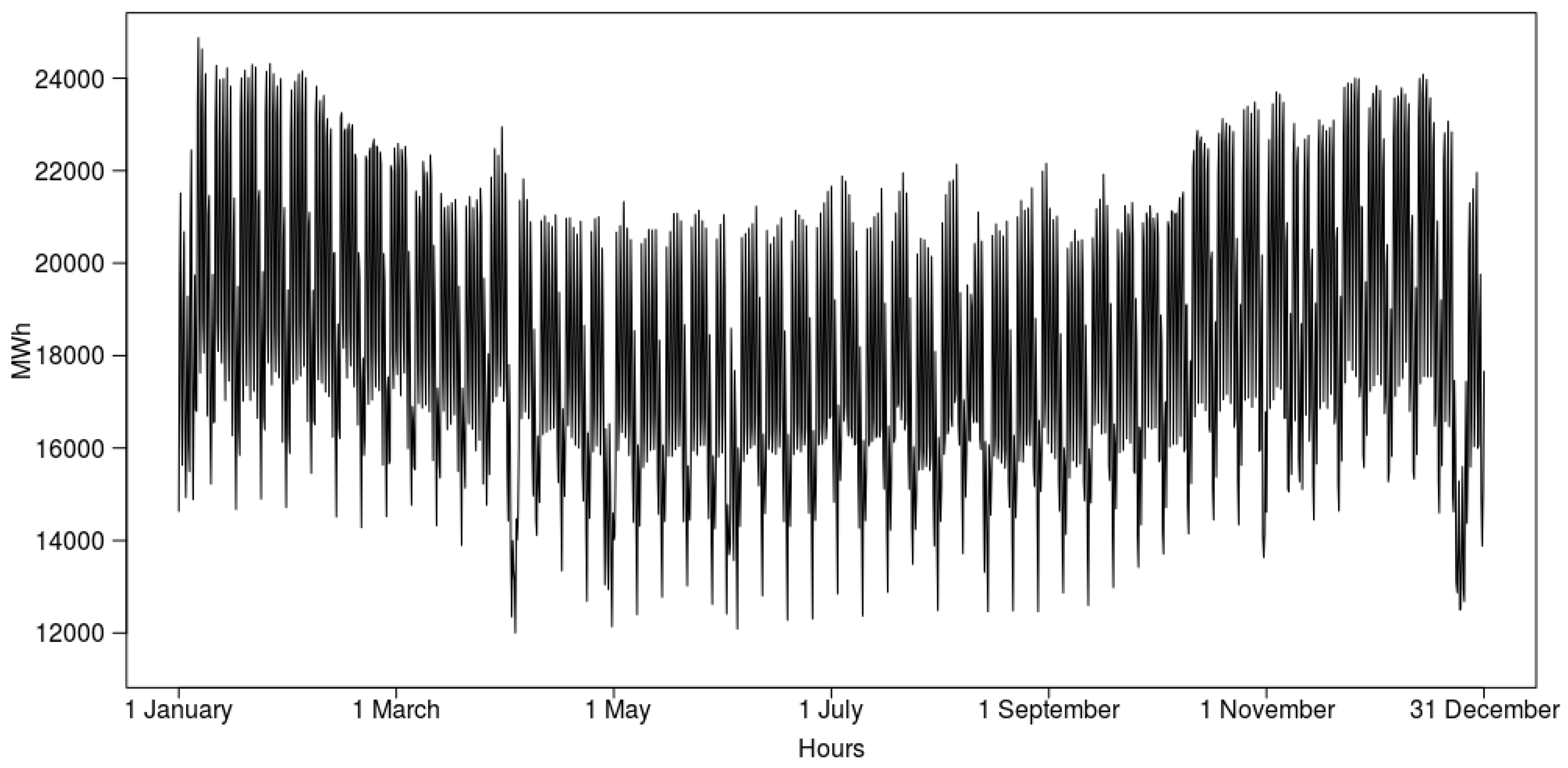
Figure 2.
Daily dynamics of the hourly load data from 9 (Monday) to 15 (Sunday) November 2015.

Figure 3.
Weekly average temperature and humidity data in Warsaw in 2015.

Figure 4.
Peak identification in the load data based on the 90th quantile of the weekly load distribution (November 2015 data).
Figure 4.
Peak identification in the load data based on the 90th quantile of the weekly load distribution (November 2015 data).

Figure 5.
Design of the two-stage modeling approach.
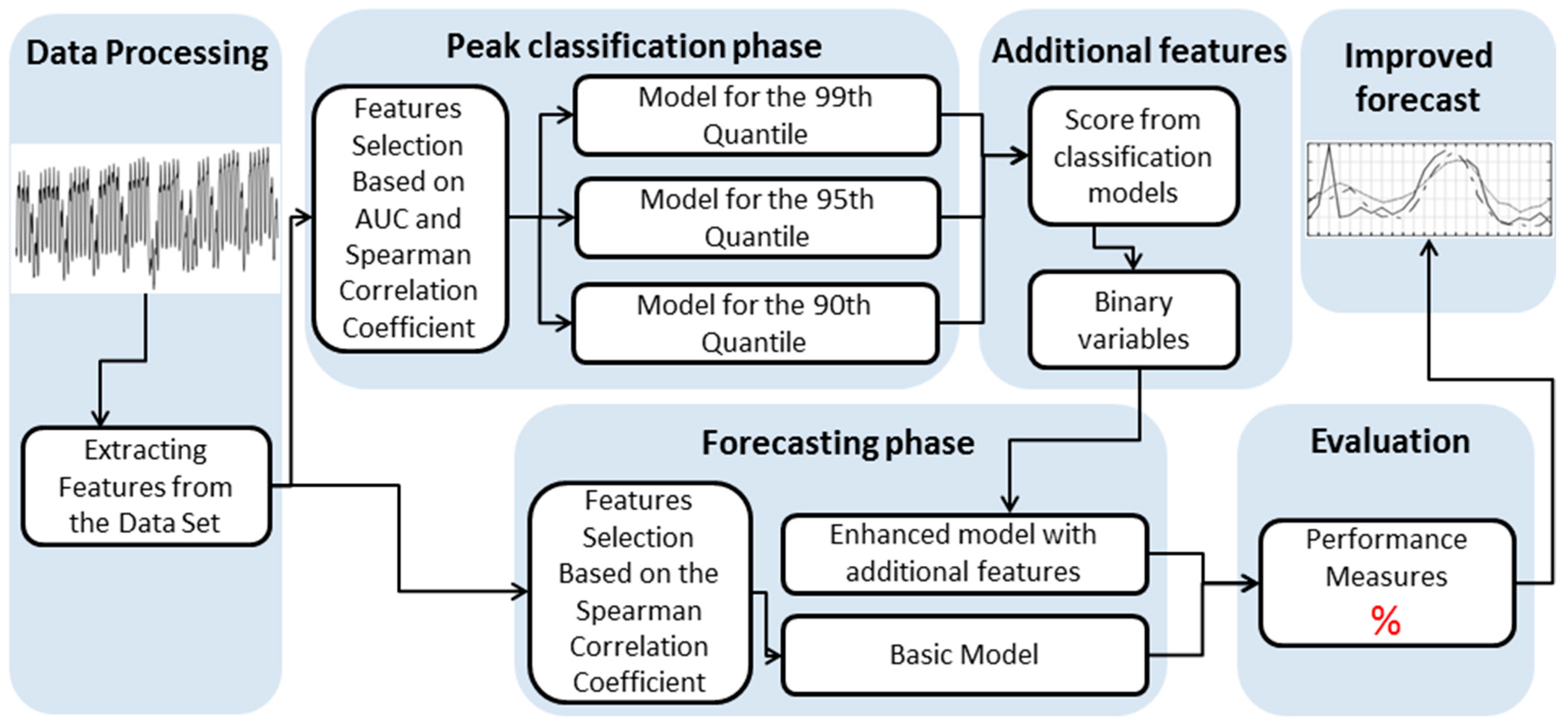
Figure 6.
ANN peaks identification in the load data exceeding the 90th quantile of the distribution (October 2015 data).
Figure 6.
ANN peaks identification in the load data exceeding the 90th quantile of the distribution (October 2015 data).
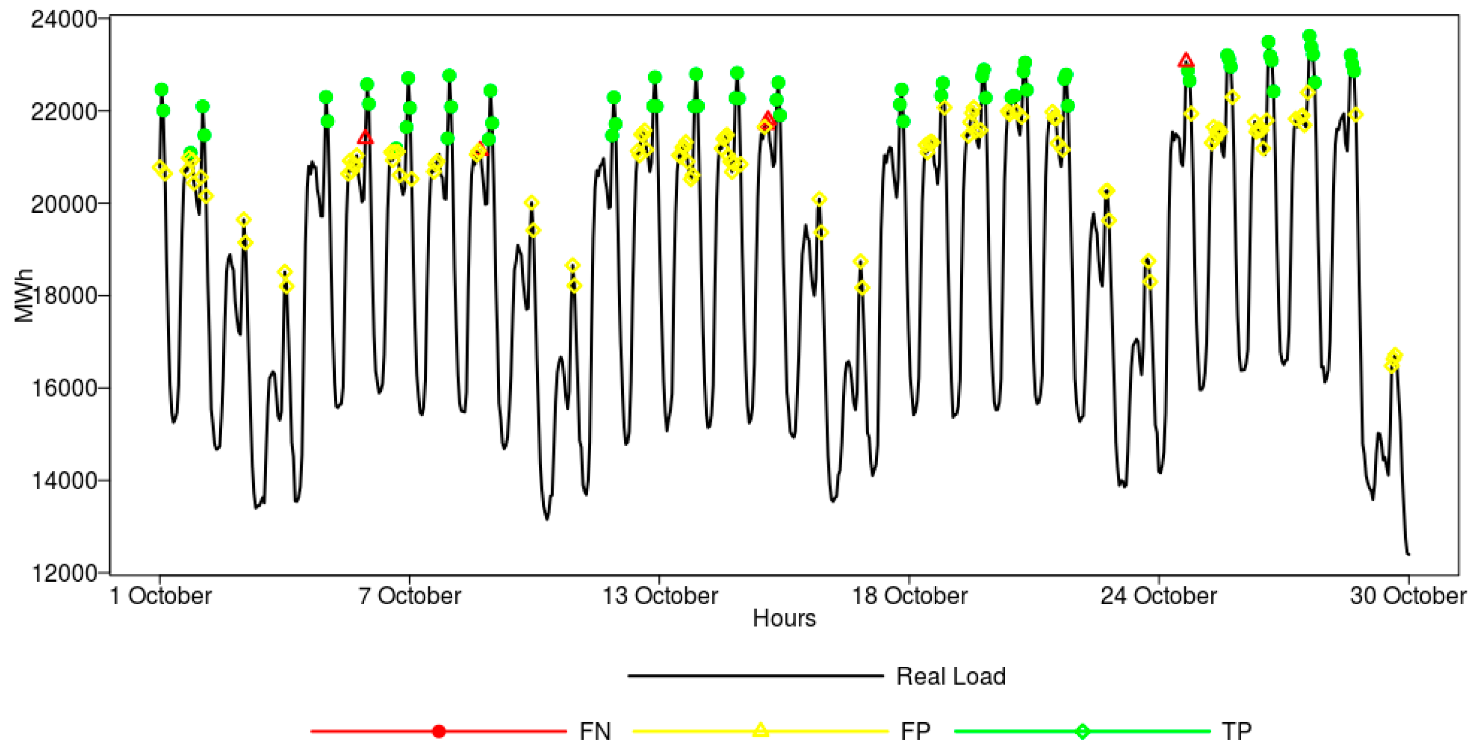
Figure 7.
Forecasting results of the base model and the improved ANN model (enhanced by peak classification data) covering October 2015 data.
Figure 7.
Forecasting results of the base model and the improved ANN model (enhanced by peak classification data) covering October 2015 data.


Table 1.
Feature vector used for estimating the models.
| Attribute No. | Description | Formula |
|---|---|---|
| 1–24 | Load of the previous 24 h | , |
| 25–32 | Average load observed over previous hourly intervals | |
| 33–38 | Load in the same hour of the previous week | , |
| 39–46 | Linear trend of the load observed over previous hourly intervals | |
| 47–54 | Average temperature observed over previous hours | |
| 55–62 | Average temperature observed over previous hourly intervals | |
| 63–70 | Average humidity observed over previous hours | |
| 71–78 | Average humidity observed over previous hourly intervals | |
| 79–83 | Hour indicator (bit encoding) | , |
| 84–88 | Day of the month indicator (bit encoding) | , |
| 89–91 | Day of the week indicator (bit encoding) | , |
| 92–95 | Month indicator (bit encoding) | , |
| 96 | Holiday indicator (dummy variable) | |
| 97 | Sunset indicator (dummy variable) |
Table 2.
Area under the curve (AUC) values for the quantitative variables used to detect 99th percentile peaks.
Table 2.
Area under the curve (AUC) values for the quantitative variables used to detect 99th percentile peaks.
| Variable Name | AUC | Variable Name | AUC | Variable Name | AUC | Variable Name | AUC |
|---|---|---|---|---|---|---|---|
| t_1 | 0.744 | t_21 | 0.551 | d_2 | 0.677 | temp_avg_19_21 | 0.530 |
| t_2 | 0.678 | t_22 | 0.629 | d_3 | 0.673 | temp_avg_22_24 | 0.496 |
| t_3 | 0.663 | t_23 | 0.689 | d_4 | 0.740 | hum_avg_1_3 | 0.615 |
| t_4 | 0.665 | t_24 | 0.720 | d_5 | 0.815 | hum_avg_4_6 | 0.650 |
| t_5 | 0.644 | temp_1_3 | 0.528 | d_6 | 0.840 | hum_avg_7_9 | 0.557 |
| t_6 | 0.608 | temp_1_6 | 0.540 | d_7 | 0.766 | hum_avg_10_12 | 0.556 |
| t_7 | 0.560 | temp_1_9 | 0.532 | avg_1_3 | 0.701 | hum_avg_13_15 | 0.610 |
| t_8 | 0.531 | temp_1_12 | 0.514 | avg_4_6 | 0.641 | hum_avg_16_18 | 0.582 |
| t_9 | 0.514 | temp_1_15 | 0.504 | avg_7_9 | 0.535 | hum_avg_19_21 | 0.508 |
| t_10 | 0.514 | temp_1_18 | 0.514 | avg_10_12 | 0.575 | hum_avg_22_24 | 0.552 |
| t_11 | 0.573 | temp_1_21 | 0.516 | avg_13_15 | 0.709 | trend_1_3 | 0.752 |
| t_12 | 0.638 | temp_1_24 | 0.514 | avg_16_18 | 0.688 | trend_1_6 | 0.632 |
| t_13 | 0.687 | hum_1_3 | 0.615 | avg_19_21 | 0.529 | trend_1_9 | 0.657 |
| t_14 | 0.714 | hum_1_6 | 0.638 | avg_22_24 | 0.684 | trend_1_12 | 0.725 |
| t_15 | 0.708 | hum_1_9 | 0.619 | temp_avg_1_3 | 0.528 | trend_1_15 | 0.786 |
| t_16 | 0.696 | hum_1_12 | 0.578 | temp_avg_4_6 | 0.549 | trend_1_18 | 0.788 |
| t_17 | 0.690 | hum_1_15 | 0.540 | temp_avg_7_9 | 0.509 | trend_1_21 | 0.731 |
| t_18 | 0.664 | hum_1_18 | 0.517 | temp_avg_10_12 | 0.543 | trend_1_24 | 0.607 |
| t_19 | 0.608 | hum_1_21 | 0.513 | temp_avg_13_15 | 0.571 | ||
| t_20 | 0.530 | wilg_1_24 | 0.519 | temp_avg_16_18 | 0.564 |
Table 3.
AUC values for the categorical variables used to detect 99th percentile peaks.
| Variable Name | AUC |
|---|---|
| month | 0.504 |
| month_day | 0.509 |
| hour | 0.748 |
| week_day | 0.678 |
Table 4.
Final set of independent variables for classification models.
| Variable Name |
|---|
| d_6 |
| trend_1_18 |
| trend_1_3 |
| d_4 |
| trend_1_12 |
| t_24 |
| t_14 |
| avg_1_3 |
| t_18 |
| hum_avg_4_6 |
| hum_avg_13_15 |
| hour |
| week_day |
Table 5.
The results of the Spearman correlation coefficient for the quantitative variables.
| Variable Name | Value | Variable Name | Value | Variable Name | Value | Variable Name | Value |
|---|---|---|---|---|---|---|---|
| t_1 | 0.7488 | t_21 | 0.4011 | d_2 | 0.5692 | temp_avg_19_21 | −0.3106 |
| t_2 | 0.6561 | t_22 | 0.5068 | d_3 | 0.5634 | temp_avg_22_24 | −0.2411 |
| t_3 | 0.5362 | t_23 | 0.5861 | d_4 | 0.5944 | hum_avg_1_3 | −0.1002 |
| t_4 | 0.4086 | t_24 | 0.6152 | d_5 | 0.7418 | hum_avg_4_6 | −0.0085 |
| t_5 | 0.2838 | temp_1_3 | −0.2290 | d_6 | 0.9082 | hum_avg_7_9 | 0.1404 |
| t_6 | 0.1697 | temp_1_6 | −0.2501 | d_7 | 0.7308 | hum_avg_10_12 | 0.2920 |
| t_7 | 0.0729 | temp_1_9 | −0.2821 | avg_1_3 | 0.6616 | hum_avg_13_15 | 0.3528 |
| t_8 | 0.0002 | temp_1_12 | −0.3190 | avg_4_6 | 0.2929 | hum_avg_16_18 | 0.2601 |
| t_9 | −0.0457 | temp_1_15 | −0.3487 | avg_7_9 | 0.0075 | hum_avg_19_21 | 0.0646 |
| t_10 | −0.0685 | temp_1_18 | −0.3611 | avg_10_12 | −0.0797 | hum_avg_22_24 | −0.0801 |
| t_11 | −0.0785 | temp_1_21 | −0.3560 | avg_13_15 | −0.0989 | trend_1_3 | −0.4443 |
| t_12 | −0.0854 | temp_1_24 | −0.3428 | avg_16_18 | −0.0013 | trend_1_6 | −0.5942 |
| t_13 | −0.0940 | hum_1_3 | −0.1002 | avg_19_21 | 0.2939 | trend_1_9 | −0.6253 |
| t_14 | −0.1003 | hum_1_6 | −0.0582 | avg_22_24 | 0.5829 | trend_1_12 | −0.5817 |
| t_15 | −0.0951 | hum_1_9 | 0.0117 | temp_avg_1_3 | −0.2290 | trend_1_15 | −0.5229 |
| t_16 | −0.0667 | hum_1_12 | 0.0996 | temp_avg_4_6 | −0.2700 | trend_1_18 | −0.4314 |
| t_17 | −0.0100 | hum_1_15 | 0.1735 | temp_avg_7_9 | −0.3406 | trend_1_21 | −0.2519 |
| t_18 | 0.0729 | hum_1_18 | 0.2053 | temp_avg_10_12 | −0.4146 | trend_1_24 | −0.0196 |
| t_19 | 0.1742 | hum_1_21 | 0.1942 | temp_avg_13_15 | −0.4455 | ||
| t_20 | 0.2865 | wilg_1_24 | 0.1643 | temp_avg_16_18 | −0.4028 |
Table 6.
Final set of independent variables for forecasting models.
| Variable Name | |
|---|---|
| hour_1 | day_week_1 |
| hour_2 | day_week _2 |
| hour_3 | day_week _3 |
| hour_4 | sunset |
| hour_5 | d_6 |
| month_1 | t_24 |
| month_2 | trend_1_6 |
| month_3 | trend_1_12 |
| month_4 | t_3 |
| day_month_1 | temp_avg_13_15 |
| day_month_2 | hum_avg_13_15 |
| day_month_3 | t_19 |
| day_month_4 | t_14 |
| day_month_5 | hum_1_3 |
Table 7.
Confusion matrix for binary classification.
| Predicted Value | |||
|---|---|---|---|
| Positive (P) | Negative (N) | ||
| Real value | Positive (P) | True positive (TP) | False negative (FN) |
| Negative (N) | False positive (FP) | True negative (TN) | |
Table 8.
Peak classification results of the machine learning algorithms. AC: accuracy; ANN: artificial neural network; RF: random forest; SVM: support vector machine.
Table 8.
Peak classification results of the machine learning algorithms. AC: accuracy; ANN: artificial neural network; RF: random forest; SVM: support vector machine.
| Training/Validation/Test Sample | |||||
|---|---|---|---|---|---|
| AC | AUC | Sens | Spec | ||
| Model for 99th percentile | ANN (iteration = 25, neurons = 7) | 0.899/0.894/0.884 | 0.969/0.967/0.968 | 0.957/0.958/0.963 | 0.898/0.893/0.885 |
| RF (mtry = 3) | 0.848/0.878/0.812 | 0.936/0.936/0.938 | 0.909/0.909/0.932 | 0.847/0.847/0.847 | |
| SVM (kernel = polynomial, degree = 2, C = 0.5, gamma = 0.5) | 0.916/0.905/0.906 | 0.981/0.966/0.971 | 0.966/0.968/0.932 | 0.915/0.904/0.904 | |
| Benchmarking model | 0.984/0.981/0.983 | 0.668/0.617/0.644 | 0.345/0.245/0.297 | 0.922/0.990/0.991 | |
| Model for 95th percentile | ANN (iteration = 27, neurons = 7) | 0.898/0.893/0.889 | 0.967/0.967/0.961 | 0.936/0.938/0.922 | 0.897/0.891/0.891 |
| RF (mtry = 3) | 0.892/0.905/0.884 | 0.949/0.954/0.962 | 0.886/0.949/0.933 | 0.893/0.86/0.860 | |
| SVM (kernel = polynomial, degree = 3, C = 1, gamma = 0.5) | 0.9259/0.9141/0.906 | 0.983/0.982/0.969 | 0.948/0.966/0.914 | 0.925/0.911/0.911 | |
| Benchmarking model | 0.957/0.955/0.954 | 0.792/0.782/0.777 | 0.607/0.587/0.578 | 0.977/0.976/0.975 | |
| Model for 90th percentile | ANN (iteration = 26, neurons = 14) | 0.902/0.889/0.879 | 0.966/0.963/0.962 | 0.902/0.89/0.908 | 0.903/0.889/0.883 |
| RF (mtry = 3) | 0.863/0.883/0.847 | 0.950/0.947/0.963 | 0.898/0.972/0.945 | 0.860/0.792/0.792 | |
| SVM (kernel = polynomial, degree = 3, C = 1, gamma = 1) | 0.922/0.908/0.892 | 0.980/0.977/0.967 | 0.977/0.935/0.899 | 0.921/0.906/0.906 | |
| Benchmarking model | 0.939/0.934/0.935 | 0.834/0.822/0.825 | 0.702/0.680/0.687 | 0.966/0.963/0.963 | |
Table 9.
Forecasting results of the machine learning algorithms.
| Training/Validation/Test Sample | ||||||
|---|---|---|---|---|---|---|
| MAPE (%) | SMAPE (%) | r-MAPE (%) | RMSE | |||
| Artificial neural network | Base model (iteration = 69, neurons = 12, decay = 0.1) | Estimate | 2.90 */3.09 */3.30 * | 2.86 */3.08 */3.27 * | 2.34 */2.50 */2.80 * | 865.2 */952.6 */895.7 * |
| Lower confidence | 2.87/2.99/3.19 | 2.83/2.99/3.20 | 2.32/2.45/2.75 | 849.5/913.8/857.0 | ||
| Upper confidence | 2.93/3.19/3.40 | 2.89/3.17/3.34 | 2.36/2.55/2.85 | 880.8/992.1/935.5 | ||
| Improved model (iteration = 86, neurons = 15, decay = 0.15) | Estimate | 2.81 */2.88 */3.10 * | 2.73 */2.91 */3.11 * | 2.19 */2.31 */2.70 * | 786.4 */866.8 */800.9 | |
| Lower confidence | 2.77/2.78/3.01 | 2.70/2.84/3.01 | 2.17/2.25/2.66 | 770.1/828.4/763.7 | ||
| Upper confidence | 2.85/2.98/3.18 | 2.76/2.99/3.19 | 2.21/2.36/2.75 | 800.3/903.2/836.4 | ||
| Random Forest | Base model (mtry = 3) | Estimate | 2.30 */3.11/3.35 | 2.25 */3.06/3.33 * | 1.66 */2.28 */2.70 | 698.9/921.5/937.8 |
| Lower confidence | 2.27/3.01/3.25 | 2.21/2.97/3.26 | 1.64/2.22/2.65 | 684.1/883.8/901.1 | ||
| Upper confidence | 2.33/3.21/3.45 | 2.27/3.14/3.41 | 1.68/2.34/2.75 | 713.6/955.4/972.6 | ||
| Improved model (mtry = 10) | Estimate | 2.21 */3.01/3.20 | 2.16 */2.95/3.17 * | 1.56 */2.16 */2.53 | 697.6/914.4/920.9 | |
| Lower confidence | 2.17/2.92/3.11 | 2.12/2.88/3.07 | 1.55/2.11/2.47 | 680.3/880.1/893.7 | ||
| Upper confidence | 2.25/3.11/3.28 | 2.19/3.04/3.25 | 1.58/2.22/2.79 | 715.7/947.5/951.2 | ||
| Support vector machine | Base model (kernel = polynomial, degree = 3, eps = 1, gamma = 1) | Estimate | 3.24 */3.45 */3.58 | 3.15 */3.39 */3.54 | 2.44 */2.58 */2.89 | 899.7/983.1/956.7 |
| Lower confidence | 3.20/3.34/3.49 | 3.11/3.30/3.44 | 2.42/2.53/2.84 | 882.8/944.7/915.8 | ||
| Upper confidence | 3.29/3.56/3.67 | 3.18/3.47/3.64 | 2.47/2.63/2.93 | 916.3/1020.3/995.8 | ||
| Improved model (kernel = polynomial, degree = 3, eps = 1, gamma = 1) | Estimate | 2.98 */3.20 */3.45 | 2.89 */3.14 */3.40 | 2.20 */2.35 */2.81 | 882.4/963.2/971.7 | |
| Lower confidence | 2.94/3.09/3.36 | 2.86/3.05/3.31 | 2.18/2.29/2.76 | 865.8/926.2/931.8 | ||
| Upper confidence | 3.03/3.31/3.54 | 2.93/3.22/3.50 | 2.22/2.39/2.85 | 898.9/999.2/1010.3 | ||
| Benchmarking model (Similar day method) | Estimate | 5.38/5.22/4.97 | 5.20/5.01/4.75 | 3.84/3.58/3.49 | 1494.5/1517.6/1458.5 | |
| Lower confidence | 5.31/5.05/4.82 | 5.14/4.86/4.59 | 3.80/3.46/3.39 | 1477.7/1463.2/1407.7 | ||
| Upper confidence | 5.45/5.39/5.10 | 5.26/5.18/4.91 | 3.89/3.67/3.58 | 1512.9/1576.6/1510.8 | ||
1 Asterisk (*) denotes significant differences (at p < 0.05) of the forecasts estimates between the base and the improved model, for the respective algorithm. MAPE: mean absolute percentage error; SMAPE: symmetric mean absolute percentage error; r-MAPE: resistant mean absolute percentage error; RMSE: root-mean-squared error.
© 2017 by the authors. Licensee MDPI, Basel, Switzerland. This article is an open access article distributed under the terms and conditions of the Creative Commons Attribution (CC BY) license (http://creativecommons.org/licenses/by/4.0/).
Share and Cite
MDPI and ACS Style
Gajowniczek, K.; Ząbkowski, T. Two-Stage Electricity Demand Modeling Using Machine Learning Algorithms. Energies 2017, 10, 1547. https://doi.org/10.3390/en10101547
AMA Style
Gajowniczek K, Ząbkowski T. Two-Stage Electricity Demand Modeling Using Machine Learning Algorithms. Energies. 2017; 10(10):1547. https://doi.org/10.3390/en10101547
Chicago/Turabian StyleGajowniczek, Krzysztof, and Tomasz Ząbkowski. 2017. "Two-Stage Electricity Demand Modeling Using Machine Learning Algorithms" Energies 10, no. 10: 1547. https://doi.org/10.3390/en10101547
Note that from the first issue of 2016, this journal uses article numbers instead of page numbers. See further details here.