Towards Cost and Comfort Based Hybrid Optimization for Residential Load Scheduling in a Smart Grid

Abstract

In a smart grid, several optimization techniques have been developed to schedule load in the residential area. Most of these techniques aim at minimizing the energy consumption cost and the comfort of electricity consumer. Conversely, maintaining a balance between two conflicting objectives: energy consumption cost and user comfort is still a challenging task. Therefore, in this paper, we aim to minimize the electricity cost and user discomfort while taking into account the peak energy consumption. In this regard, we implement and analyse the performance of a traditional dynamic programming (DP) technique and two heuristic optimization techniques: genetic algorithm (GA) and binary particle swarm optimization (BPSO) for residential load management. Based on these techniques, we propose a hybrid scheme named GAPSO for residential load scheduling, so as to optimize the desired objective function. In order to alleviate the complexity of the problem, the multi dimensional knapsack is used to ensure that the load of electricity consumer will not escalate during peak hours. The proposed model is evaluated based on two pricing schemes: day-ahead and critical peak pricing for single and multiple days. Furthermore, feasible regions are calculated and analysed to develop a relationship between power consumption, electricity cost, and user discomfort. The simulation results are compared with GA, BPSO and DP, and validate that the proposed hybrid scheme reflects substantial savings in electricity bills with minimum user discomfort. Moreover, results also show a phenomenal reduction in peak power consumption.

1. Introduction

It has been observed that the residential area is a major cause of energy consumption and greenhouse gas (GHG) emissions. In China, it is considered the second highest sector which is responsible for energy consumption and GHG emission. Around $40\%$ of energy is consumed by the residential sectors in Arabian countries. While, In Palestine $60\%$ of energy is consumed [1]. With the emergence of new types of demand (i.e., electric vehicles, smart appliances etc.) and economic development in the past couple of decades, a drastic increase in the energy consumption by the residential area has been noticed [2]. This shows that the residential sector has a significant role in energy consumption which in turn threatens the reliability and efficiency of the power grid. To fulfil the increasing demand, there is a need to install bulk generation and transmission infrastructure, which is a very cumbersome and expensive process. The electricity market has also increased the electricity prices in response to increased user demand. The concept of smart grid (SG) has emerged which introduces information and communication technology in the traditional grid infrastructure.

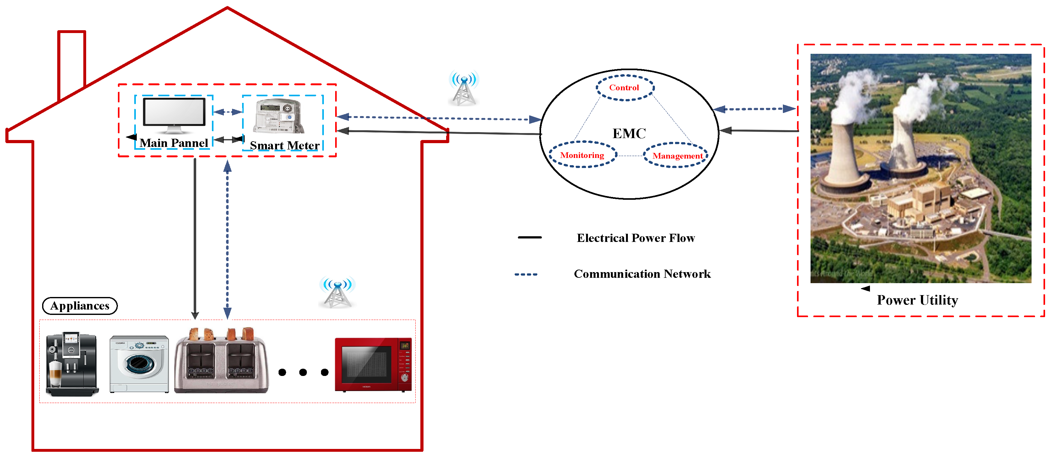
A smart home plays a very vital role to overcome the above mentioned challenges. It is equipped with smart appliances, smart meter and an energy management controller (EMC). Basically, the main motives behind the utilization of energy management programs include environmental concerns, capacity limits and reliability of utility infrastructure systems, maintainance and operation, and to meet the financial needs of consumers. The energy management in entire electrical network is classified into two categories: supply side management (SSM) and demand side management (DSM). The SSM is responsible for generating and delivering reliable energy to the consumers. Conversely, DSM utilizes the potential of advance communication and control infrastructure. It is one of the key components of the SG that aims at utilizing the available energy effectively and optimally. DSM designs demand response (DR) programs which entice the consumers to actively participate in load shifting mechanism in response to time varying prices. By shifting laod from on-peak to off-peak hours, the electricity consumer achieves significant reduction in cost but has to tolerate the discomfort in the form of delayed operation of appliances [3].

In the literature, a lot of efforts have been done to tackle the above mentioned challenges. We categorise the literature review into two main threads. In the first thread, we will discuss the concerns related to the minimization of electricity cost, peak load and users’ discomfort. Rastegar et al. in [4] proposed an idea of cost minimization along with the value of lost load (VOLL). The idea behind VOLL is to enhance the consumers’ priorities and minimize the difference between the actual and the predetermined energy consumption of appliances. Authors in [5,6] considered energy cost as an objective function to be optimized by efficiently utilizing the available energy. The trade-off analysis between privacy and cost is addressed in [7], whereas [8] demonstrated a trade-off between consumers’ comfort and operation delay of devices. In [9], Vardakas et al. uses the recursive process for peak load calculation. The authors develop four control scenarios under real-time pricing (RTP) environment. Ref. [10] considered user satisfaction in the proposed approach while restricting the total cost under the predefined budget. However, in this approach, devices with high power ratings are neglected. The results validate that the proposed models have efficiently and optimally reduced the electricity consumption cost of the consumers. In [11,12], the proposed techniques aim to minimize the energy consumption cost while taking into account the users’ convenience. Thermal comfort is taken as a metric of users’ satisfaction in the proposed work. Muralitharan et al. in [13] aim to minimize the consumption cost while considering the waiting time of consumers. ToU pricing mechanism is used in the proposed scheme. The results validate the trade-off between cost and waiting time of consumers. In [14], the authors developed a novel concept of cost efficiency (CE): the ratio of total energy consumption benefits to the total electricity payments. CE is considered as an indicator for consumers to adjust their energy consumption pattern. Moreover, the effects of DERs and service fee on CE are analyzed. The performance results show that CE is increased with increasing DERs and decreased with increasing service fee. Authors in [15] designed a model to minimize the consumption cost and balance the energy consumption under ToU pricing scheme. Moreover, renewable and storage systems are efficiently addressed, so in this way the surplus energy can be sold back to the grid. Zhang et al. [16] proposed a model to minimize the electricity cost and reduce carbon emission. A cluster of 30 houses is taken under consideration and each house having 12 devices subjected to control. In [17] authors deal with the problem of unanticipated peaks. In [18,19,20,21,22], electricity consumption cost and operational delay of devices are addressed as an optimization problem. Minimization of end users’ electricity consumption cost and comfort maximization are the two conflicting objectives to achieve, simultaneously.

While in the second thread, we discuss the scheduling techniques used for managing energy in the smart homes. In DSM, several optimization techniques exist to efficiently manage the energy consumption behavior of consumers. Many researchers focused at both mathematical and heuristic optimization techniques which are capable to optimally schedule the consumers’ load. In [10,23,24], the authors applied genetic algorithm (GA) as an optimization technique, in which electricity cost is taken as a primary objective function to be minimized. The MINLP along with dynamic pricing scheme is used in [25] to manage energy in a smart home. Bahrami et al. in [26] approximate the users’ optimal scheduling policy by using Markov perfect equilibrium (MPE). The authors have developed an online load scheduling learning (LSL) algorithm which helps to determine the users’ MPE policy. Samadi et al. in [27] propose a novel real-time pricing algorithm for the future smart grid by creating an interaction between smart meters and energy providers and exchanging the real-time price and energy consumption information of subscribers’. In [28,29], residential load scheduling problem is solved by using MINLP. In [30], the authors used game theoretic approach for cost minimization problem, whereas in [31], a variant of ant colony optimization (ACO) is used to solve the energy management problem. Yi et al. in [18] proposed an opportunistic based optimal stopping rule (OSR) for scheduling of home appliances. Chakraborty et al. [32] devised a system for energy optimization by the integration of Photovoltaic (PV) and a wind turbine as renewable energy sources (RESs) In order to address uncertainties occurred by RESs integration fuzzy logic is considered. For optimal scheduling and dispatching of energy, an efficient quantum evolutionary algorithm (EA) is implemented while considering the economic and environmental impacts. Moreover, scheduling is performed optimally in order to alleviate the cost of production and carbon emission resource. In [33], the authors have used the optimization techniques: teacher learning based optimization (TLBO) and shuffled frog leap (SFL) to efficiently manage energy in smart home. MILP is applied in [34] and [35] for efficient utilization of available energy. Gupta et al. in [34] proposed a model based on cost minimization problem. MILP is used for problem formulation, whereas, load scheduling is performed via genetic algorithm (GA). Authors in [36] developed a dynamic model for home energy management system (HEMS). The developed model employs the game theoretic approach for efficient scheduling of residential load. Safdarian et al. in [37] categorized DSM infrastructure into two stages. In first stage, decentralized system is considered and the aim is to minimize the electricity cost of consumers. MILP is used to formulate the problem and is solved by using general algebraic modeling system (GAMS). In second stage, the aim of the proposed model is to benefice the utility by modifying the load profile while preserving the constraints of cost and comfort. Mixed integer quadratic programming is used to achieve the objective of modifying load profile curve. In [38], the authors proposed a model based on a large number of residential appliances. PL-Generalized Bender’s technique is used for scheduling the residential load and protecting the private information of the consumers. This model efficiently handled the consumption cost of the residential consumers along with the protection of privacy. The interval number optimization technique is proposed in [39] to handle residential load scheduling problem, thermostatically controlled and interruptible loads are considered in this scheme. Moreover, BPSO combined with integer linear programming (ILP) is used for load scheduling.

In the literature, as discussed earlier, zillion of methods are introduced for efficient utilization of available energy by using DSM infrastructure. The entire electrical network can be made well balanced and reliable, by managing the energy consumption, electricity cost, peak to average ration (PAR) and users’ satisfaction. The work discussed above addresses the challenges of electricity consumption cost, consumers’ convenience and peak demand reduction. However, some of the challenges are yet to be addressed by the research community; both by industry and academia. The real time implementation of the current system still requires a lot of advanced research efforts. Dynamic and adaptive control systems should be developed to predict and monitor the energy consumption behavior of occupants, comfort level of consumers and more importantly, stability of the entire grid. In [40,41], authors proposed a model for the scheduling of large number of devices with an objective of cost minimization and reduction of peak power consumption. Load scheduling strategy is applied in order to achieve an optimal energy consumption pattern. Evolutionary algorithm (EA) is implemented to apportion the consumers’ load aptly over the time horizon. The proposed models perform well in terms of cost minimization and peak demand reduction, however, consumers’ comfort is not addressed, which is a key component for end users’ to participate in DR programs. In [42], minimization of electricity consumption cost and user discomfort are considered as an objective function. Time flexible and power flexible appliances are considered for efficient utilization of energy. The scheduling problem is formulated as convex optimization and electricity price is defined by the utility on day ahead basis. The simulations results show that the proposed technique achieved a desire trade-off between both the parameters of an objective function. However, by increasing the size of problem the computational complexity also increases. In order to address these challenges: cost and discomfort minimization along with peak demand reduction, a hybrid technique is proposed. The contributions of this paper are as follows:

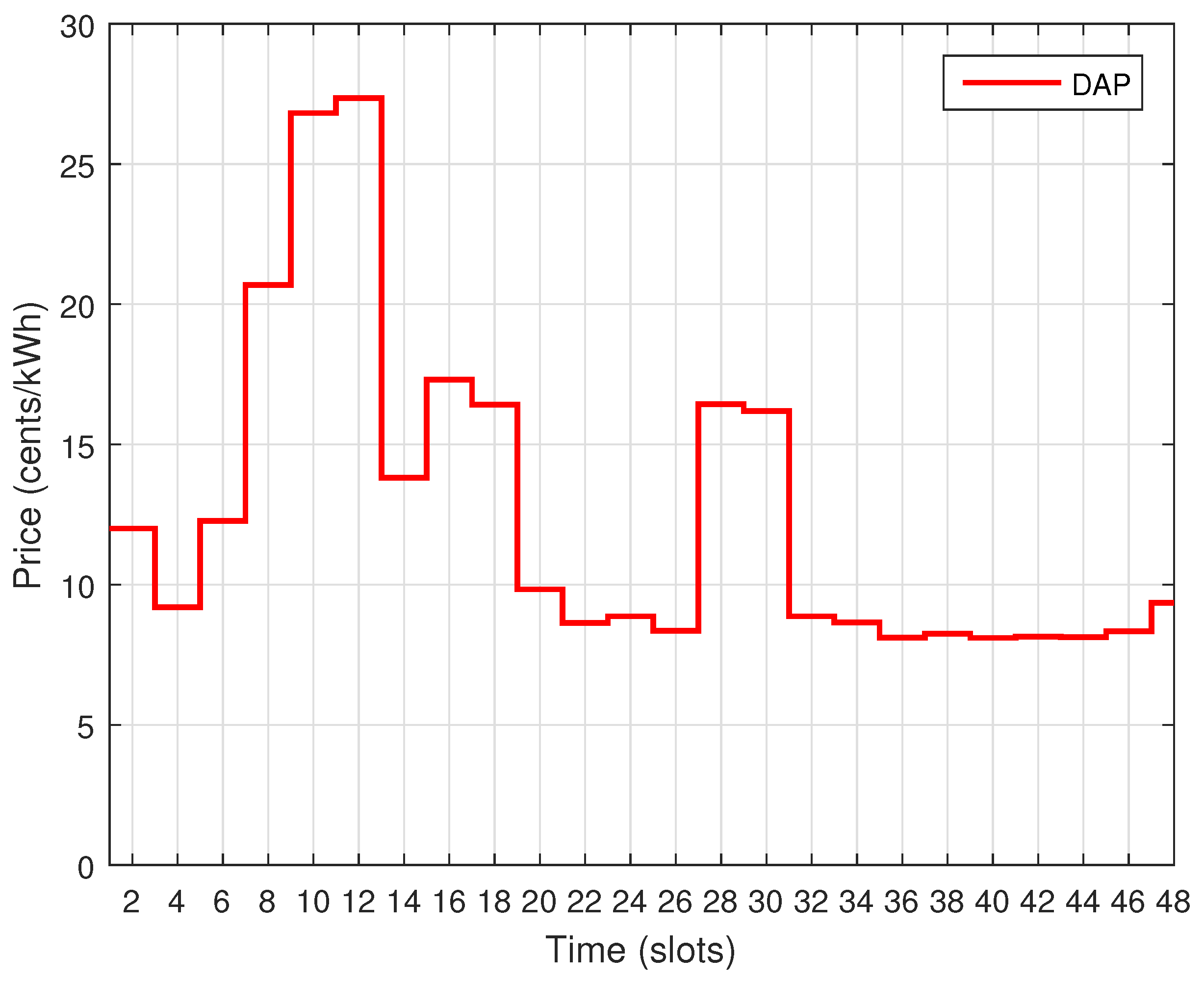
• GAPSO: In this paper, we focus on designing a load shifting technique with day-ahead pricing (DAP) mechanism. We demonstrate the performance of a traditional optimization technique and two heuristic optimization techniques. After analyzing GA and BPSO, it is observed that these techniques show pre mature convergence when dealing with high dimension problems. So, there is a need to develop such an optimization method which can improve search efficiency and precision and adequate to handle multiple constraints. Based on these heuristic techniques, a hybrid technique is proposed with the objectives of cost and discomfort minimization. Extensive simulations are conducted to validate the results. The efficiency of the proposed technique is validated by analyzing the performance metrics, which show high cost savings with minimum user discomfort. Furthermore, our proposed model has less computational complexity and more generality.
• We formulate the binary optimization problem through multiple knapsack problem (MKP). MKP helps in the effort of finding an optimal solution while employing GAPSO and respecting the total capacity of available amount of power.

The rest of the paper is organized as follows. Section 2 elaborates the system model. The problem formulation is briefly discussed in Section 3. Heuristic optimization techniques used in this work is given in Section 4. In Section 5 proposed technique is discussed. Section 6 contains simulations and discussions. Section 7 concludes the work.

2. System Model

In this research work, we consider multiple smart homes in a residential area where the appliances in each smart home have low energy consumption ratings and short length of operation. There are 2604 controllable appliances available in this sector from 14 different types of appliances. All types of appliances have different energy consumption pattern and operation time. As in this area consumers have low priorities regarding the time when the energy has to be utilized, so more savings can be achieved in residential sector. The amount of incentives given to consumers depend on how much discomfort the consumer is willing to undergo. In the proposed model, we considered shiftable appliances. However, devices fulfill their length of operation time without exceeding the maximum allowable delay. Additionally, in the proposed model comfort level of consumer is incorporated, as a result of which the consumption cost is increased. Moreover, half an hour time slot is considered in the proposed model. The power ratings of appliances and their length of operation are given in

Table 1. Appliances parameters.

Appliance’s Type	Power Rating (kW)	Length of Operation Time (hours)	Total Devices
Dryer	1.2	4.0	189
Dish Washer	0.7	3.0	288
Washing Machine	2.0	2.5	268
Oven	1.3	3.0	279
Iron	1.0	2.0	340
Vacuum Cleaner	2.0	2.0	158
Fan	0.2	24	288
Kettle	2.0	4.0	406
Toaster	0.9	3.0	048
Rice Cooker	0.85	4.0	059
Hair Dryer	1.5	2.0	058
Blender	0.3	1.5	066
Frying Pan	1.1	1.5	101
Coffee Maker	0.8	1.5	056
Total	-	-	2604

.

The system model comprises of energy management controller, smart homes, communication networks and pricing model. The system model is demonstrated in Figure 1.

2.1. Energy Management Controller

In this model, DSM focuses on efficient utilization of energy in residential sector. The power utility is directly connected to EMC and exchanges bidirectional information and unidirectional power flow in real time.The central EMC receives the price information from the power utility and performs the appropriate action. At the same time it contains the information from the consumer’s end. It acts as a gate way between power utility and several homes. The main functionalities of EMC are monitoring, controlling and managing the residential load. In this case DSM uses load shifting as a basic scheme that can be implemented by using the central EMC. In this way EMC is capable to handle large number of residential appliances in well informed and organized manner. The residential devices send their arrival requests to the EMC and then requests are processed based on the availability of time slot. The scheduling mechanism is performed on day ahead basis.

2.2. Communication Network

The communication network includes wide area networks (WANs), neighbourhood area networks (NANs) and home area networks (HANs). The residential appliances are connected to smart meter via HANs. The residential appliances share their information to the smart meter and then this information is forwarded to the central EMC. The smart meters of different homes are connected to the central EMC via NANs. Through NANs the collective information is reached to the main EMC. The EMC exchanges the received information to the power utility via WANs. Through WANs the demand response and the price information is exchanged between power utility and the main EMC.

2.3. Pricing Schemes

In this work two pricing schemes are used, and based on these schemes we analyzed the performance of our proposed model.

2.3.1. DAP Model

The basic purpose of providing the pricing model on day ahead basis is to facilitate the consumers to take well-informed decisions. In this way consumers can adjust their electricity consumption pattern while taking care of comfort level. This helps consumers to reduce their electricity bills and these pricing models are readily available to consumers via advanced metering infrastructure. In this work, DAP is used similar to [41], and is shown in Figure 2. The pricing signal portrays three main regions: on-peak, off-peak and shoulder-peak hours. The load can be altered by observing the pricing signal offered by the utility.

2.3.2. CPP Model

To validate and generalize the performance of the proposed model, we extend our approach by implementing the critical peak pricing (CPP) for load scheduling purpose. In CPP, depending upon the utility policies, electricity prices are double or even higher at critical peak hours. More specifically in this case we have considered a hot summer day, having critical peak hours from 12:00 p.m. to 3:00 p.m. where prices are almost double than usual. Critical events occurred very rarely in entire season or a year due to intense hot or cold weather. Figure 3 portrays the CPP pricing signal.

3. Problem Formulation

In this section, energy scheduling problem is formulated for an objective function and constraints. The aim is to minimize the consumption cost and maximize the users’ comfort while respecting all the constraints. In objective function we formulate the maximization of user comfort as minimization of user discomfort, so both the terms are used interchangeably.

3.1. Multiple Knapsack Problem

The energy scheduling is one of the core issues in energy management system. In this work, multiple knapsack problem (MKP) is used to address the scheduling problem of a residential load. Knapsack is a combinatorial problem in which a number of objects, each having weight and value, must be packed in a bin of a specific capacity, in such a way that the total profit inside the bin is maximum. MKP is a resource allocation problem, and every resource has a specific capacity constraint. In this way, the system finds an optimal combination of household appliances operation modes while respecting the total capacity of available amount of power [43]. The reasons for using MKP are as follows,

• It can be referred as a simplest integer linear programming (LP).
• It can be viewed as subproblems in many complex problems.
• It may represent the great practical situations.

For the sake of simplicity the abbreviations used in mathematical formulation are given in

Table 2. Abbreviations.

Variables	Description
T	Time period of a day
$T_u^t$	User defined time
$T_s^t$	Scheduler defined time
$EMC$	Energy Management Controller
${\lambda }_i$	Electricity price
$T_{OTI}^i$	Operation time interval of appliance i
${\alpha }_i$	Start time of an appliance i
${\beta }_i$	End time of an appliance
$T_{LoT}^i$	Length of operation time of device i
$Ca{p}_T$	Maximum allowable energy that can be used for each hour of the day

.

3.2. MKP in Energy Management System

The relation between the key terms used in MKP and energy management system can be developed as in [44] and is given below,

• m knapsacks = m time interval.
• n objects = n appliances.
• w weight of an object = $E_i$ Energy consumed by an appliance i.
• value of an object = consumption cost of an appliance at time t.
• Capacity of knapsack = user demand with respect to the maximum amount of energy that can be drawn from the grid at time t.

The mathematical formulation of an objective function and constraints is performed and the performance metrics of the considered problem are computed.

The electricity consumption cost, consumers’ discomfort, total energy consumption and PAR are calculated and based on these equations we modelled the proposed approach and addressed the challenges of residential load.

The energy consumed by a single residential device over 24 h time horizon can be calculated by using the following equation,

$${\displaystyle E=\sum _{t=1}^m{P}_r^i\times {\Delta }_{i,t}}$$

(1)

where $P_r^i$ is power rating of a device i and ${\Delta }_{i,t}$ is status of device i at time slot t which can be given as,

$${\Delta }_{i,t}=\left\{\begin{array}{cc}\hfill 1& \mathrm{if}\mathrm{device}\mathrm{of}\mathrm{type}i\mathrm{at}\mathrm{time}t\mathrm{is}\mathrm{ON};\hfill \\ \hfill 0& \mathrm{otherwise}.\hfill \end{array}\right.$$

(2)

The total residential energy consumed by n number of smart devices can be calculated as follows,

$${\displaystyle E_e^r=\sum _{t=1}^m{\displaystyle (\sum _{i=1}^n{P}_r^i\times {\Delta }_{i,t}})}$$

(3)

Similarly, the total energy consumption cost of all the devices is given by

$$C_c^r=\sum _{t=1}^m\sum _{i=1}^n{P}_r^i({\Delta }_{i,t}\times {\lambda }_t)$$

(4)

As maximizing the user comfort and minimizing the user discomfort can be used alternatively. So, for simplicity of our objective function i.e., Equation (7) , we used “minimization” for both the parameters collectively.

The consumers’ discomfort is represented as $\Gamma$ and calculated by using Equation (5) similar to [42], similarly Equation (5) also demonstrates that $\rho$ and k are the real numbers that represent the operational characteristics of devices, and $T{s}_i^t$ and $T{u}_i^t$ are the operational time of appliances set by the scheduler and consumer respectively.

$$\Gamma =\sum _{i=1}^n\rho {(T{s}_i^t-T{u}_i^t)}^k$$

(5)

where,

$$0<\rho <1,k\ge 1$$

The value of $\rho$ lies between this interval because we aim to minimize the discomfort caused by delaying the operation of appliances. In case of violation of this limit, the electricity consumer will be suffered with more discomfort in the form of more delay in the operation of appliances. Where, the real number k represents the behaviour of appliance.

PAR can be calculated as follows

$$PAR=\frac{{max}_{t\in T}({\displaystyle \sum _{i=1}^n}(P_r^i\times {\Delta }_{i,t}))}{\frac{1}{m}({\displaystyle \sum _{t=1}^m}{\displaystyle \sum _{i=1}^n}(P_r^i\times {\Delta }_{i,t}))}\forall T=\{1,2,\dots ,m\}$$

(6)

We have used the linear weighted sum method (scalarization approach) in which both parameters; cost and discomfort get normalized values, range between 0 and 1. So, both cost and discomfort are comparable. Furthermore, we have assigned equal weights (i.e., 0.5) to both cost and discomfort and their sum is equal to 1, ${\omega }_1$ + ${\omega }_2$ = 1.

The mathematical formulation of an objective function and constraints can be given as,

$$\begin{array}{c}\hfill \begin{array}{c}\mathrm{Minimize}\hfill \end{array}\left({\omega }_1\times C_t^r+{\omega }_2\times \Gamma \right)\\ \hfill \begin{array}{c}\mathrm{Subject}\mathrm{to}\hfill \end{array}\end{array}$$

(7)

$$\begin{array}{c}\hfill \sum _{i=1}^n(P_r^i\times {\Delta }_{i,t})\le Ca{p}_T\forall t=\{1,2,\dots ,m\}\end{array}$$

(7a)

$$\begin{array}{c}\hfill PA{R}^{\mathrm{with}\mathrm{EMC}}\le PA{R}^{\mathrm{without}\mathrm{EMC}}\end{array}$$

(7b)

$$\begin{array}{c}\hfill {\displaystyle \sum _{t=1}^m{\Delta }_{i,t}=T_{LoT}^i\forall i=\{1,2,\dots ,n\}}\end{array}$$

(7c)

$$\begin{array}{c}\hfill {\alpha }_i\le T_{OTI}^i\le {\beta }_i\end{array}$$

(7d)

$$\begin{array}{c}\hfill C_c^{r\mathrm{with}\mathrm{EMC}}\le C_c^{r\mathrm{without}\mathrm{EMC}}\end{array}$$

(7e)

$$\begin{array}{c}\hfill E_e^{r\mathrm{with}\mathrm{EMC}}=E_e^{r\mathrm{without}\mathrm{EMC}}\end{array}$$

(7f)

Equation (7) shows an objective function to be minimized and comprises of electricity cost and discomfort of consumers. Equations (7a)–(7f) define the constraint functions. In Equation (7), the cost and user discomfort are assigned equal weights ${\omega }_1$ and ${\omega }_2$ respectively. However, the values of weights can be varied in the range between $[0,1]$ or ${\omega }_1$ + ${\omega }_2$ = 1. In Equation (7a), limit shows the maximum allowable capacity that can be utilized at any hour of the day. The boundary limit ensures the stability of a grid by restricting the consumers to a limited amount of energy consumption. In Equation (7b), PAR is addressed to avoid the peaks creation at any hour of the day so that stability of a grid remains un-jeopardized.

Equation (7c) shows that length of the operation time of each device must be completed to avoid the users’ frustration. Equation (7d) depicts that device must fulfill operation time after its start time and before end time in order to mitigate the user discomfort. In Equation (7e), it is depicted that the total consumption cost with EMC must be less than the total consumption cost without EMC. Equation (7f) illustrates that the total energy consumption with and without EMC must be the same.

4. Optimization Techniques

The optimization techniques used in this work are briefly discussed.

4.1. Heuristic Optimization Techniques

We have considered two heuristic optimization techniques. On the basis of these techniques we have proposed our own technique.

4.1.1. Brief Description of GA

GA has been successfully used in problems such as scheduling job shops and travelling salesman. It is a robust adaptive optimization technique which is based on biological paradigm. It performs efficient search on-poorly defined spaces which motivates the application of this technique to solve the binary optimization problem. It aims at finding the best candidates from the entire population. The fittest candidates are ranked higher in the population, whereas the least fit candidates are ranked lower in the population. In the end, one fittest candidate is selected which is called global best. The entire chronological process is followed as, random generation of population, fitness evaluation, elitism, selection, crossover and mutation. The population is updated by using the aforementioned parameters, the fittest chromosomes are survived and least fit candidates are weeded out in the next population. More detailed knowledge about GA can be found in [45,46].

4.1.2. Brief Description of BPSO

BPSO is an established version of PSO, it is a heuristic optimization technique inspired by the social behavior of bird flocking and fish schooling. This technique has been extensively used for a variety of binary optimization problems which motivated us to solve our binary optimization problem employing this technique. BPSO aims at finding the best possible solution to a problem from entire search space. The velocity and position of particles are randomly initialized, then updated by using their respective equations. The particles traverse through the entire space so that an optimal solution can be found. The evaluation of all the particles are performed and the global best and personal best positions are updated if required. At the end of stipulated iterations one global best is opted which is considered as a solution to the problem [47]. Each particle is associated with its position and velocity. The position of particle at any point in search space can be determined as follows:

$${\overrightarrow{X}}_k\left(t\right)={\overrightarrow{X}}_k(t-1)+{\overrightarrow{V}}_k\left(t\right)$$

(8)

Each particle is associated with the velocity vector, containing the information of local and global best positions achieved so far. The updated velocity of a particle can be given as,

$$\begin{array}{c}\hfill {\overrightarrow{V}}_k\left(t\right)=\phi {\overrightarrow{V}}_k(t-1)+{\Omega }_1.rand1.({\overrightarrow{P}}_k-{\overrightarrow{X}}_k(t-1))\\ \hfill +{\Omega }_2.rand2.({\overrightarrow{P}}_g-{\overrightarrow{X}}_k(t-1))\end{array}$$

(9)

where $\phi$ is the inertia constant or weight of the particles, $k\in 1,2,\dots ,M$ is the number of particles, ${\Omega }_1$ and ${\Omega }_2$ are constant numbers and ${\Omega }_1$ + ${\Omega }_2$ = 4. ${\overrightarrow{P}}_k$ and ${\overrightarrow{P}}_g$ are local and global best solutions achieved so far. ${\overrightarrow{X}}_k(t-1)$ and ${\overrightarrow{X}}_k\left(t\right)$ are previous and current positions of particle in the search space.

The velocity update expression composed of three main components.

• The first component is often known as “inertia” or “momentum”, it tends to move a particle in the same direction as it was travelling in. The inertia component can be scaled with a constant factor known as inertia constant. The inertia constant controls the velocity of a particle so that the particle cannot move beyond or below the scope of optimal search space. Mathematically inertia constant can be given as,

  $$\phi ={\phi }_f+({\phi }_f-{\phi }_i)\times \left(\frac{k^{th}iteration}{maximumiterations}\right)$$

  (10)
• The second component represents the local best solution found for the first time in search space. It tends to converge the solution toward local optima.
• The third component can be referred as the linear attraction towards the global best solution from the entire search space. It tends to fetch the optimum solution by using group knowledge of all the particles.

If the value of velocity exceeds the maximum or minimum limits, then it can be written as follows:

$${\overrightarrow{V}}_k\left(t\right)=\left\{\begin{array}{cc}{\overrightarrow{V}}_{max}\hfill & \mathrm{if}{\overrightarrow{V}}_k\left(t\right)>{\overrightarrow{V}}_{max};\hfill \\ {\overrightarrow{V}}_{min}\hfill & \mathrm{if}{\overrightarrow{V}}_k\left(t\right)<{\overrightarrow{V}}_{min}.\hfill \end{array}\right.$$

(11)

The position of each member of particle is updated by using the following equation,

$${\overrightarrow{X}}_k\left(t\right)=\left\{\begin{array}{cc}1\hfill & \mathrm{if}\mathrm{sig}({\overrightarrow{V}}_k\left(t\right)>rand);\hfill \\ 0\hfill & \mathrm{otherwise}.\hfill \end{array}\right.$$

(12)

where, $sig({\overrightarrow{V}}_k\left(t\right))=\frac{1}{(1+exp({\overrightarrow{V}}_k\left(t\right))).}$

Sigmoid function converts the value of velocity to a binary format by comparing it with randomly generated number in range between $[0,1]$. The maximum and minimum extremes of velocity are [${\overrightarrow{V}}_{max}$ and ${\overrightarrow{V}}_{min}$].

4.2. Deterministic Optimization Technique

The description of deterministic technique is given as follows:

Brief Description of DP

The dynamic programming is used in order to solve the knapsack problem. DP was basically introduced by Bellman [48] to solve the knapsack problem. It has the ability to divide a problem into sub-problems and memorizing. DP allows the knapsack problem to be divided into n sub problems. The solution of each problem is maintained in a table. In this work, small items having largest values i.e., electricity cost are selected for Off-peak hours, where large item with small values are used to represent On-peak hours.

5. Proposed Technique

Residential sector has large number of appliances of different types, and all the appliances have different power ratings and consumption patterns. DSM needs such a technique that can efficiently handle these complexities. In literature, mathematical techniques such as linear programming (LP) and DP are used for this purpose, these techniques require more computational time and additionally, inadequate to handle multiple constraints [41,49,50,51]. Evolutionary heuristic techniques have shown capabilities to cope with such complex scenarios.

GAPSO

In the beginning, two heuristic optimization techniques: GA and BPSO are implemented and their performance is analyzed. Both the heuristic optimization techniques are briefly discussed in Section 4. After analyzing the performance of these algorithms, it is observed that the two above mentioned techniques both show pre mature convergence when dealing with high dimension problems. As a result of pre mature convergence, it is difficult and even impractical to solely rely on such optimization criteria. So, there is a need to develop such an optimization method which can improve search efficiency and precision and adequate to handle multiple constraints. In this work, therefore, GAPSO is proposed so as to obviate the problem of pre mature convergence. The proposed technique is intended to solve the residential load scheduling problem in more accurate and economic way. Moreover, in comparison to traditional optimization methods, the proposed model has lower computational complexity.

The positive traits of each technique are merged together to overcome the problem of convergence at local optima. The proposed technique is then capable of searching feasible space more effectively. The steps involve in the proposed hybrid model are given as; in the beginning a random population is generated, and then evaluation of the fitness function is performed by using 7. Tournament base selection criteria is used for selecting the parents from the population. Binary crossover and two bits mutation is used in this work. The crossover and mutation is done on selected parents to modify the population. Crossover, mutation and fitness evaluation are performed similar to [52]. Elitism is the process of remembering the good solution achieved so far. At this stage, position and velocity of particles are further updated by using Equations (8) and (9) respectively. While updating the velocity, sigmoid function which is discussed in Section 4 is used to convert the values in binary format. The evolution of population by using the innate traits of BPSO: position and velocity, further explores the search space. This results in mitigating the problem of pre mature convergence. The entire process is repeated until the termination criteria is reached. The termination criteria depends on the stipulated number of iterations or when the variations in fitness are not more than a predefined limit (i.e., 10⁻¹⁰) for numerous (i.e., 50) successive generations. Algorithm 1 shows the working of the proposed technique.

In this way, the proposed scheme has significantly affected the desired performance parameters. The user comfort in term of waiting time is also taken into consideration, since it is of great importance. User comfort along with reimbursement is the only factor which enticed the consumers to actively participate in DR program. So, the proposed technique is considered to manage electricity cost and user comfort along with peak consumption. The parameters used in the proposed technique are given in

Table 3. Variables used in proposed technique.

Variables	Values
Probability of crossover	0.9
Probability of mutation	0.1
Insite	1.0
Vmax	4.0
Vmin	−4
${\Omega }_1$	2.0
${\Omega }_2$	2.0
Population size	200
Maximum Iterations	600
$\rho$	0.001
k	3.0

.

Algorithm 1: GAPSO

6. Simulations and Discussions

In this section, the performance of GA, BPSO, and GAPSO is discussed in detail. While implementing the heuristic optimization techniques for scheduling of residential load, various factors are observed regarding cost minimization, efficient power consumption, peak reduction and user comfort.

6.1. Performance Parameters Definitions

The cost minimization can be referred to as the amount of reduction in electricity bills of consumers. The consumers pay this amount to the utility on hourly consumption basis at the completion of a predefined period. The efficient power consumption can be defined as intelligent utilization of available power in such a way that the total demand never exceeds the generation capacity. Due to synchronization among consumers’ energy utilization pattern, peaks are formed which may damage the stability of a grid. The user comfort of consumers can be defined as the minimum electricity cost and minimum interruption of devices in daily routine life.

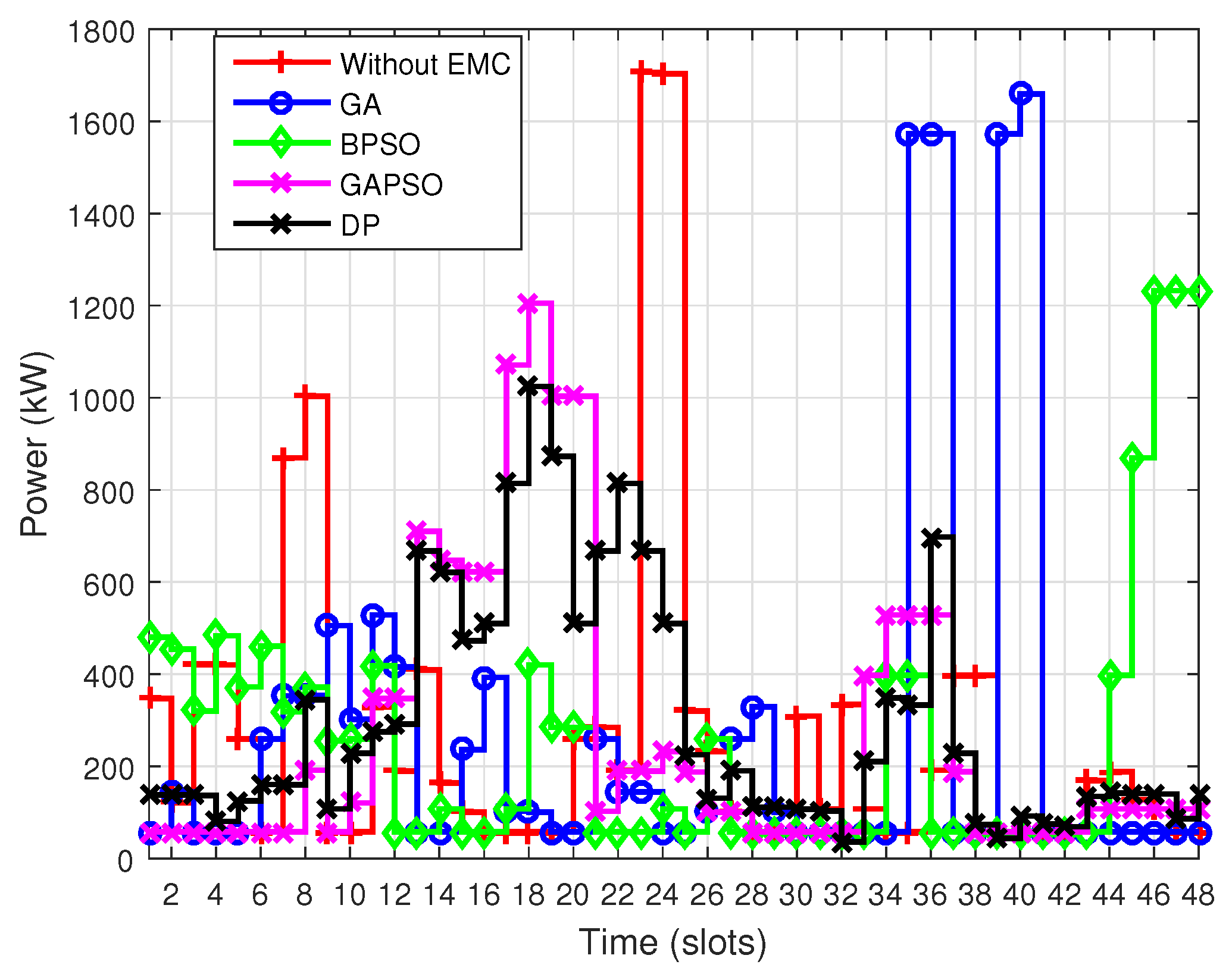
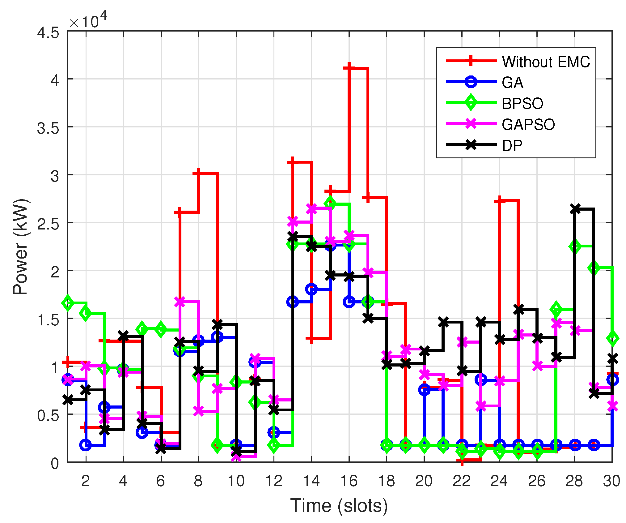
6.2. Peak Power Consumption

Figure 4 and Figure 5 show the power consumption behavior under four optimization techniques with DAP mechanism on daily and monthly basis respectively. The energy consumption depends on power rating and length of the operation time of devices. The performance of GA in term of peak power consumption is analyzed. It is demonstrated and validated that GA is less efficient when dealing with peak power consumption. This is due to the global exploration mode of GA which always focuses on minimum electricity price offered by the utility. This resulted in peaks formation at off-peak hours while user satisfaction is not taken under consideration. In this way GA scheduled most of the residential devices at hours where electricity prices are low regardless of taking peak power consumption into account. Whereas, BPSO performed well in term of reducing peak power consumption, because BPSO scheduled less number of devices at off-peak hours as compared to that of GA, this results in significant reduction in peak power consumption. In GAPSO, the peak power consumption is analyzed and it is observed that peak consumption is reduced to a significant amount. Additionally, the results of DP are also analyzed, and it is observed that DP performed better in term of peak demand reduction. It is observed that GA, BPSO, GAPSO and DP have hourly peak consumption of 1572.3 kW, 1232.3 kW, 1085.3 kW and 1108.8 kW respectively. Results validated that the proposed technique has efficient response for time varying price signal.

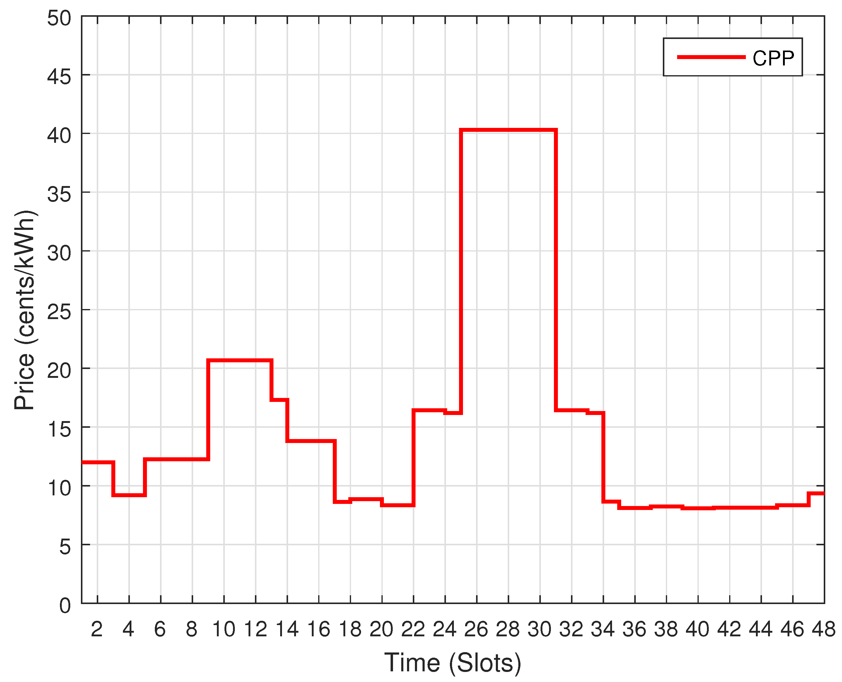
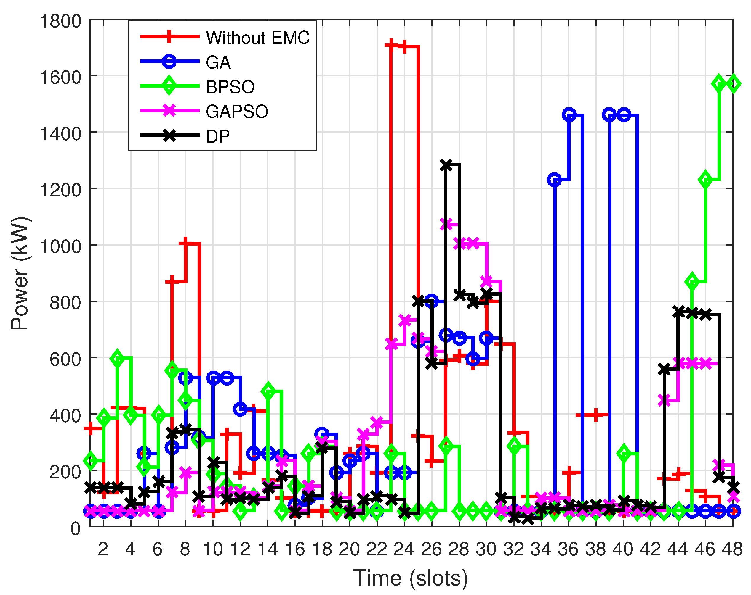
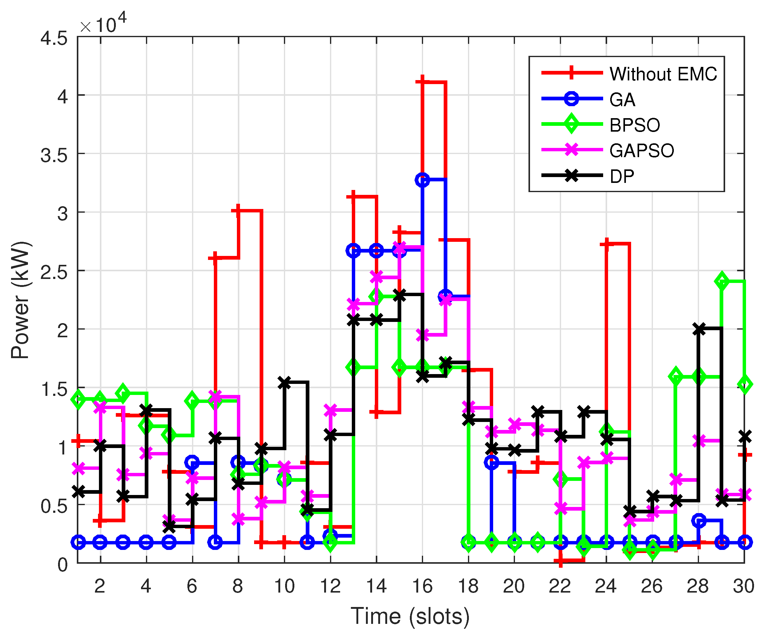
Figure 6 and Figure 7 show that the proposed scenario is implemented for CPP. For CPP, it is observed that during a hot or cold day, most of residents consume energy during critical peak hours as a result of which more peaks are created during this time. The overall residential energy consumption behavior is demonstrated in

Table 4. Daily Energy Consumption Cost and Peak Load.

Technique	Parameters	Without EMC	With EMC	Reduction (%)
GA	Cost ($)	1581.9	1480.7	29.9702
	Peak-Load (kW)	1706.3	1572.3	7.8532
BPSO	Cost ($)	1581.9	1591.2	24.0470
	Peak-Load (kW)	1706.3	1232.3	27.7794
GAPSO	Cost ($)	1581.9	1181.8	25.2923
	Peak-Load (kW)	1706.3	1085.3	36.39
DP	Cost ($)	1581.9	1297.2	25.6467
	Peak-Load (kW)	1706.3	1108.8	35.0172

and Table 6.

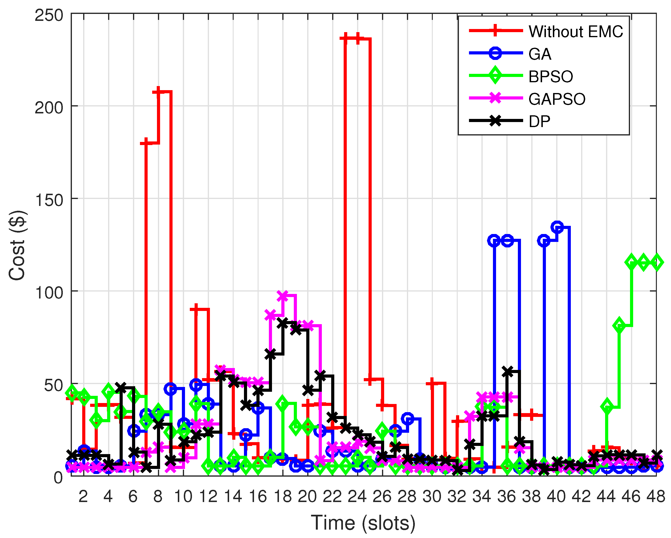
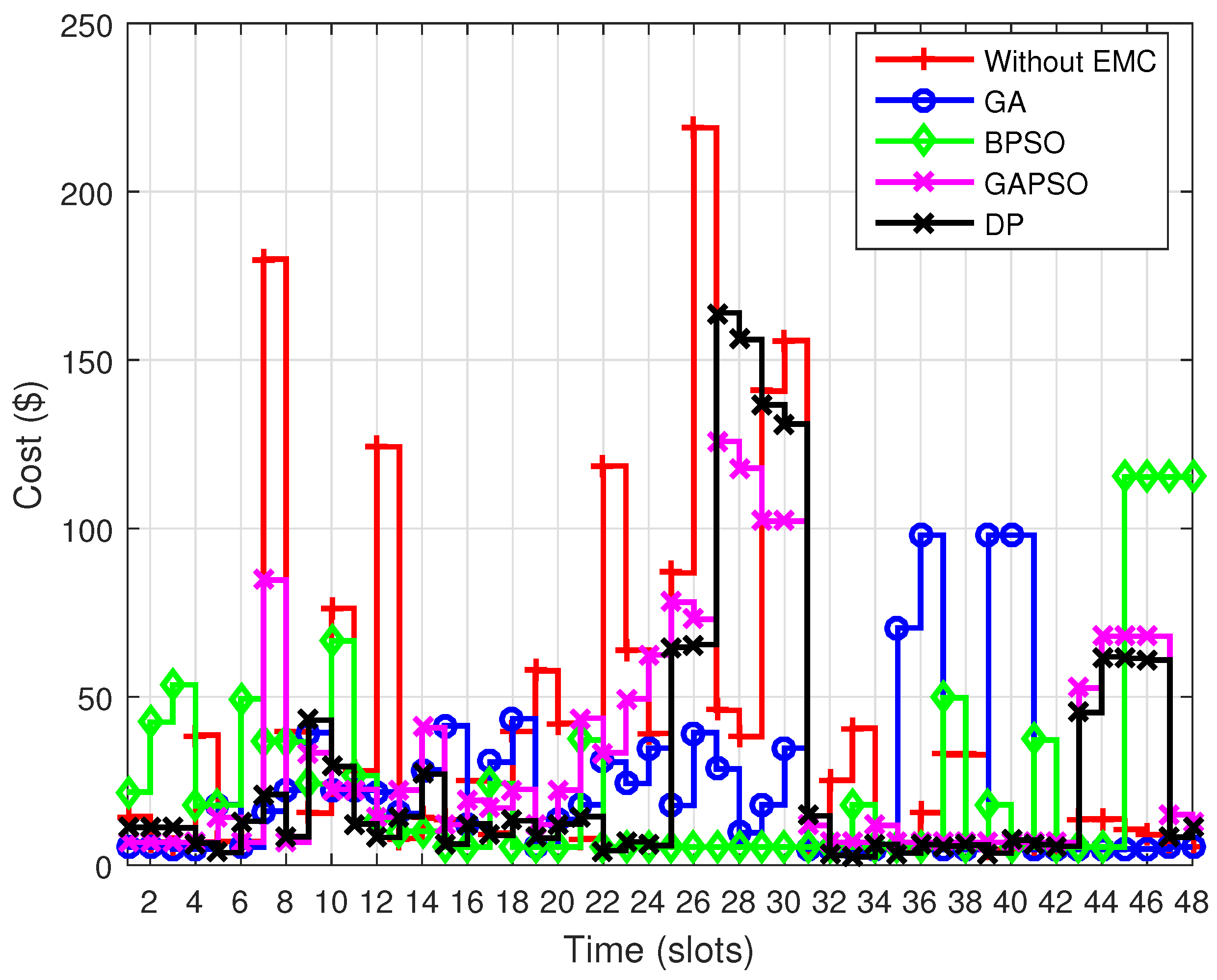
6.3. Electricity Cost

Electricity consumption cost under different techniques is demonstrated in Figure 8 and Figure 9 for DAP mechanism. It is observed from the figures that the performance of GA shows substantial savings in electricity bills. The results validate that GA achieved 29.9702% reduction in electricity consumption cost. Whereas, BPSO achieved the reduction of 24.0470% in electricity consumption cost. Because both the techniques shifted the residential load from on-peak hours to off-peak hours where prices are minimum regardless of waiting time, and hence results in reduction in electricity cost. Through out the ample simulations it is shown that GAPSO successfully managed to reduce the consumption cost up to 25.2923% with minimum waiting time. Although the proposed technique is less efficient than GA in term of cost reduction, however, with optimized consumers’ satisfaction. The reason associated with this fact is the inverse relationship between electricity bills and user satisfaction. The performance of the proposed model is also compared with DP. The results demonstrate that the proposed model has comparable performance with DP, however, with less computational complexity and storage space.

Since GA finds an optimal or near optimal solution from the entire search space and schedules the residential devices where consumers pay minimum electricity expenses. It is an inherent trait of GA that it can deal with complexities and non-linearities. It is capable of fulfilling the length of operation time of all the devices. Due to all these characteristics GA efficiently manages to reduce the electricity consumption cost. The performance of BPSO in term of cost minimization is analyzed and in this work it is shown that BPSO achieved less savings in electricity bill as compared to that of GA. It is attributed to the fact that BPSO uniformly scheduled the residential load over the time period to avoid the peaks creation. Although BPSO shifted the load at off-peak hours, however, the shifted load is comparatively less than that of GA. It is worth mentioning that by delaying an operation of devices, more reduction in electricity cost can be achieved at end consumers’. While analyzing the performance of the proposed model in terms of cost minimization, it is observed that GAPSO has optimally achieved the objective of cost minimization. The results show that GAPSO achieved 4.6779% less reduction in electricity consumption cost as compared to that of GA. Moreover, it is also observed that GAPSO achieved 1.2453% more reduction in electricity cost than BPSO, because in proposed technique both the parameters: consumption cost and user discomfort are taken into consideration. It results in fewer savings in electricity bills with improved consumers’ lifestyle. To substantiate the performance of the proposed work, results are compared with DP. It is observed that both the techniques performed efficiently while reducing the energy consumption cost. DP achieved a bit higher savings because it converges to the optimal results, however, at the expense of time and storage space.

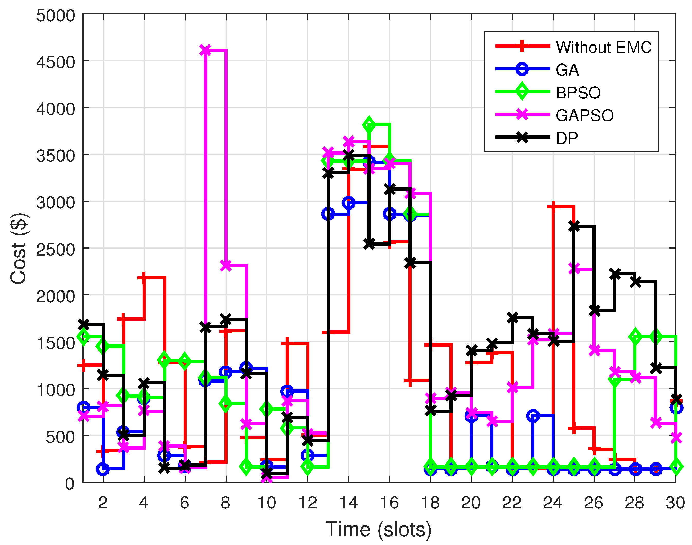
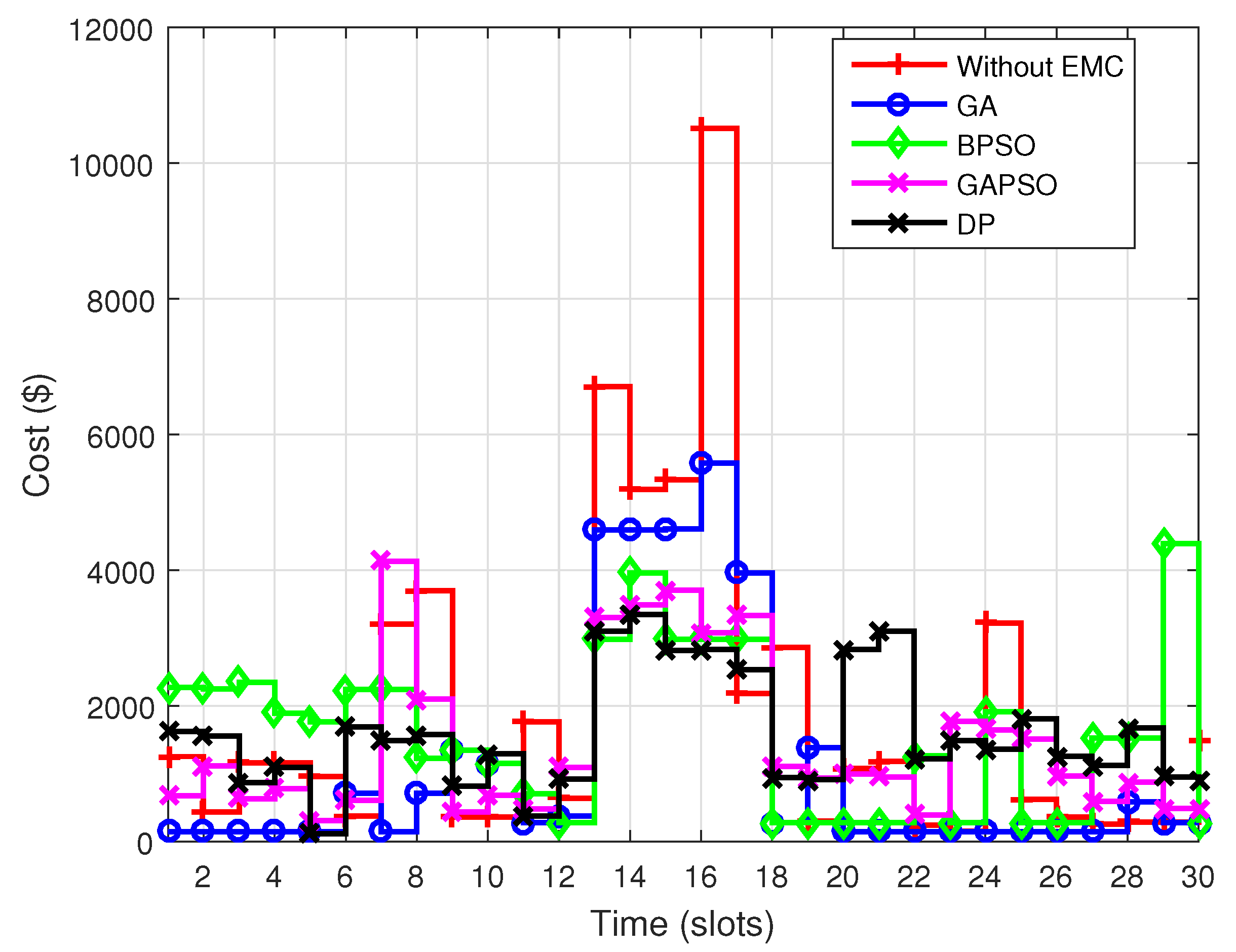
Figure 10 and Figure 11 show the energy consumption cost for CPP signal on daily and monthly basis. It is noted that during critical hours consumers are charged with high electricity prices. It is also observed that in case of CPP energy consumption cost is significantly increased as compared to that of DAP, because utility offers maximum electricity prices during critical hours (i.e., 12 p.m.–3 p.m.). Energy consumption cost is analyzed for both the scenarios in Table 4 and Table 6.

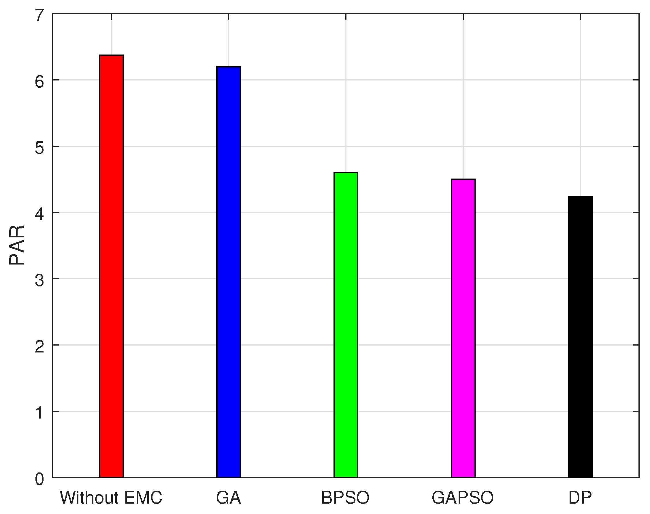
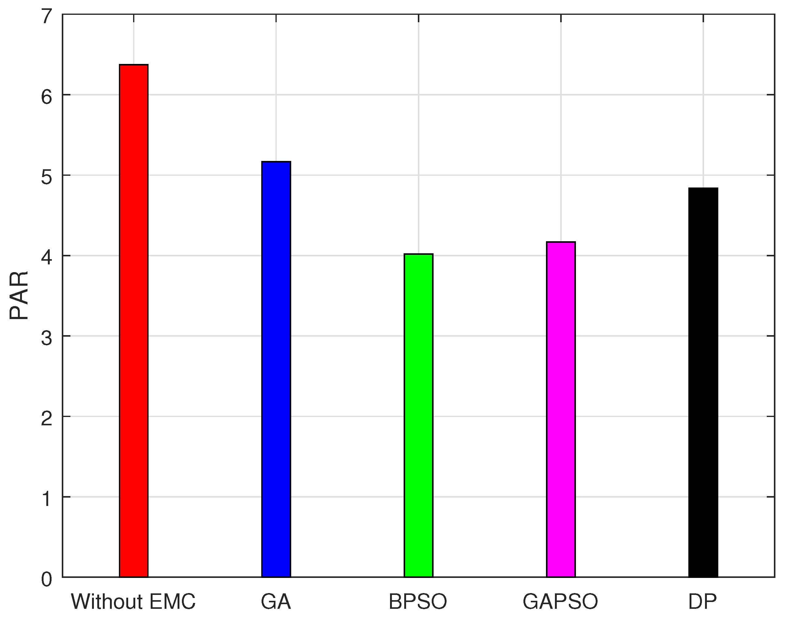
6.4. PAR

The stability and reliability of a grid can be ensured by analyzing the PAR. Figure 12 and Figure 13 depict PAR on daily and monthly basis when considering DAP as a pricing scheme. Figures infer that GA and BPSO achieved 7.8532% and 27.7794% reduction in peak power consumption respectively. Both heuristic techniques scheduled residential load from on-peak hours to off-peak hours. It is validated from the results that these heuristic techniques scheduled the load where electricity price is minimum. Whereas, GAPSO reduced 36.39% peak power consumption. This is due to the fact that GAPSO managed to distribute the entire residential load over 24 h time horizon. The load is distributed in such a manner that no peaks are created while respecting the waiting time of devices. Moreover, the performance of DP is also analyzed and compared with the proposed approach, it is observed that DP performed better in terms of peak demand reduction.

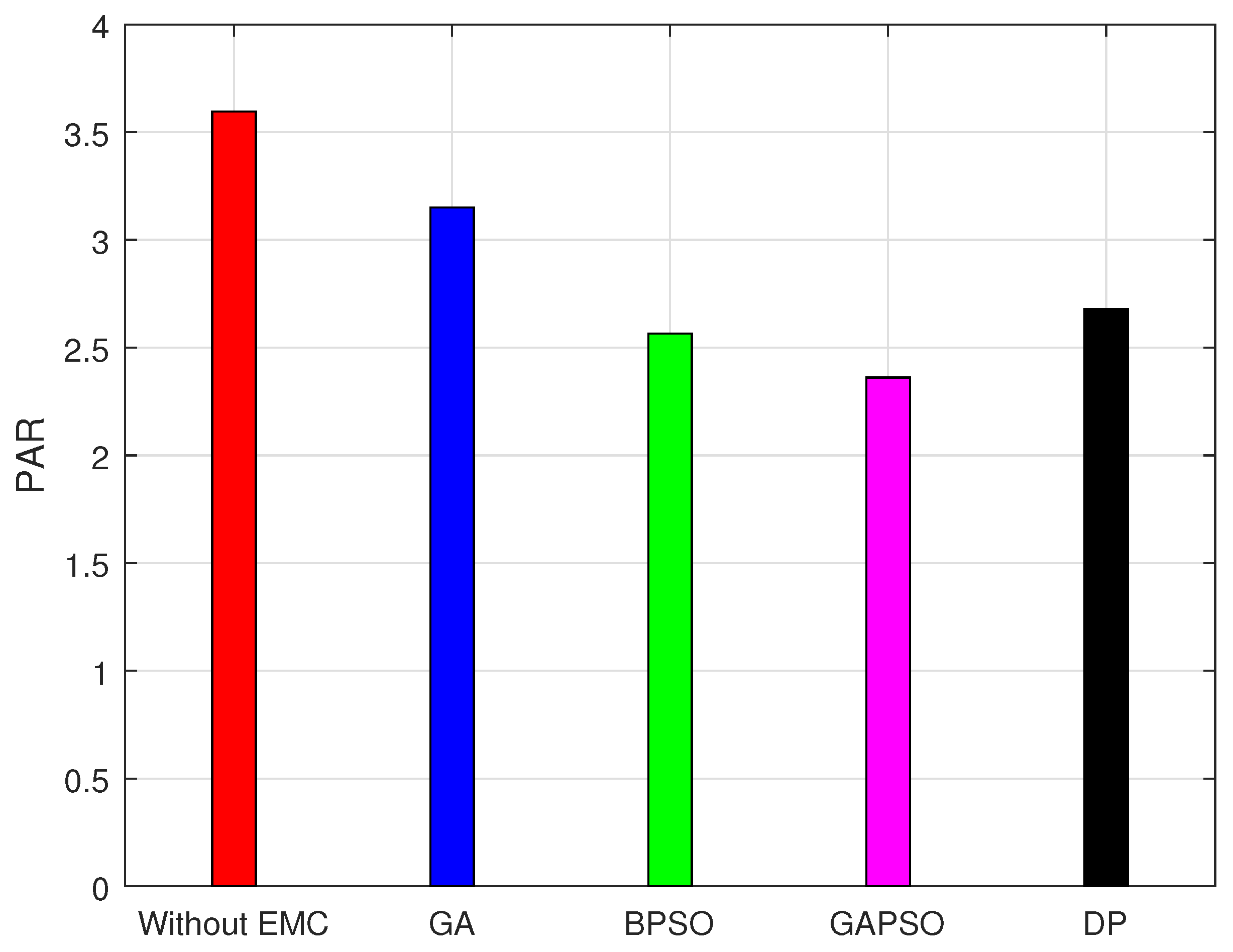
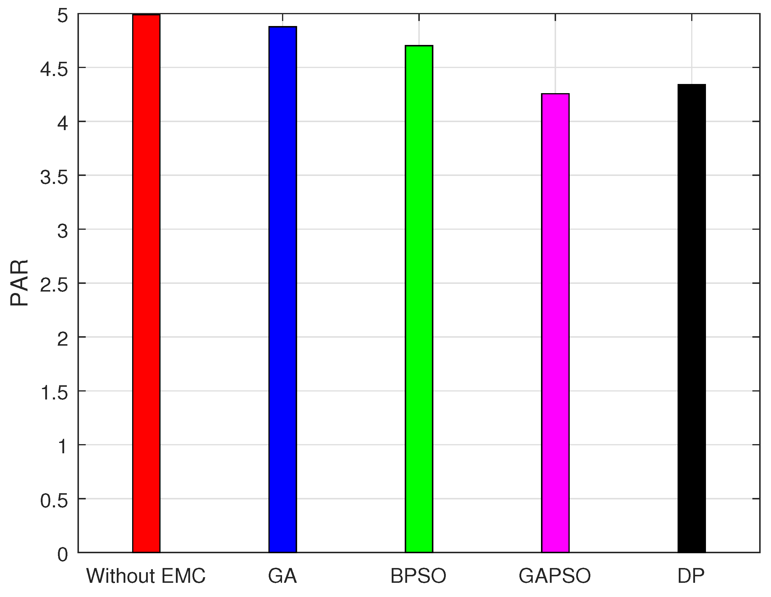
For CPP, Figure 14 and Figure 15 show the PAR for a day and a month respectively. It is deduced that for a single day, the BPSO performed well as compared to other techniques, however, GAPSO outperformed rest of the techniques when compared with rest of the techniques for a month. It is due to the fact that, GAPSO scheduled the most prior load at critical hours. So as to maintain the stability of entire electrical network during critical peak hours, while taking into account the users’ discomfort.

6.5. User Comfort

The user comfort is associated with minimum consumption cost, minimum waiting time for the operation of devices, maintaining desired indoor temperature level, illuminance level, air quality and humidity etc. In this work, waiting time is considered as user comfort and thus to be optimized. While implementing the GA for the residential load scheduling problem, user comfort is not taken into consideration. It results in maximum load scheduled at end hours and reduced maximum consumption cost. Similarly, in BPSO user comfort is not taken into consideration, and operation time of most of the devices are shifted to later hours. User comfort in terms of user discomfort and waiting time can be given as follows:

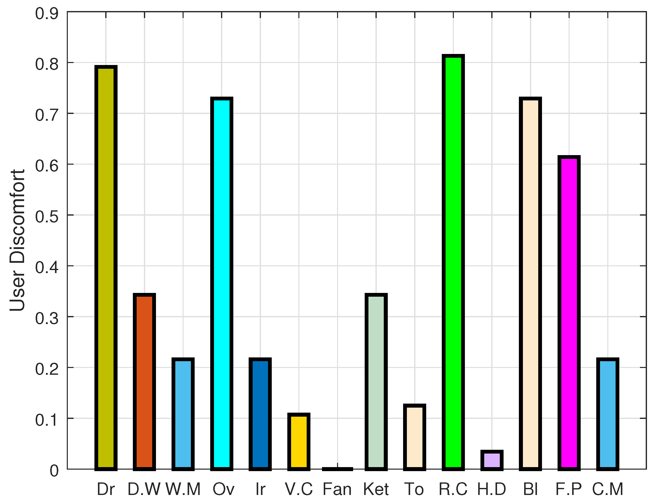
• Since in this model, the maximization of user comfort is considered equivalent to the minimization of user discomfort, so both the terms can be used interchangeably. Figure 16 portrays the user discomfort of all the residential devices over the 24 h time horizon. Through performing extensive simulations it has been noticed that by minimizing the user discomfort, electricity cost is increased. The waiting time associated with discomfort is also analyzed and discussed.
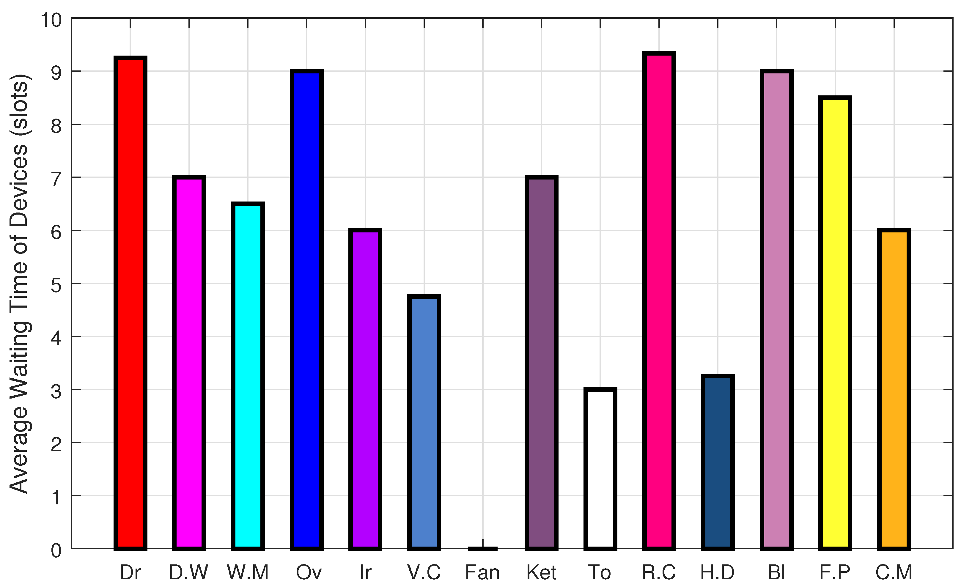
• Figure 17 demonstrates the waiting time of all the appliances. The average waiting time of 5 h is considered in the proposed scheme. Moreover, in this work, the length of operation time of fan is 24 h and it is demonstrated that the associated waiting time is zero for this device. Generally, by delaying the appliance’s operation time more monetary benefits are achieved at consumers’ end. It is also observed in the proposed technique, that with the incorporation of user comfort, comparatively less savings are achieved. In the proposed scenario half an hour is considered as an operational time slot of appliances (i.e., 1 slot = 30 min).
• Figure 16 shows the discomfort faced by each corresponding residential device. Whereas, Figure 17 shows that average waiting time for each device. No comparison is being made in these figures, as the purpose of these figures is to demonstrate the user discomfort and average waiting for each corresponding residential device.

6.6. Feasible Region

A region comprises a set of points having a possible solution for a problem is known as a feasible region. Generally, feasible region is associated with the concept of optimization. In this work, feasible region is considered as an area containing all the possible solutions for an optimization problem. The evaluated performance parameters are analyzed graphically with the help of feasible region.

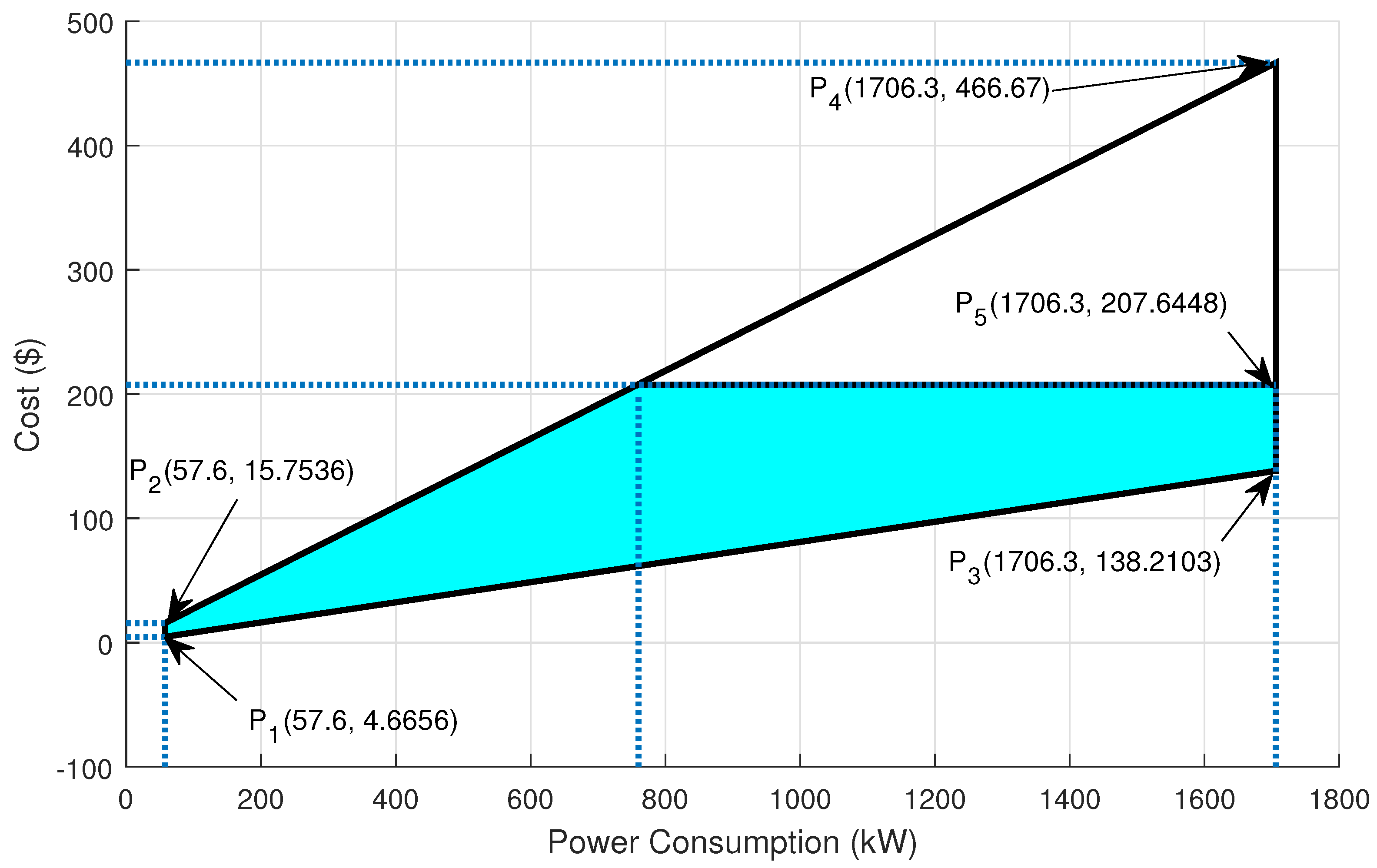
6.6.1. Feasible Region for Consumption Cost and Power

Electricity cost and power consumption are two directly linked parameters, varying consumption behavior and electricity price affect the electricity cost. A region bounded by a set of four points: P1(57.6, 4.6656), P2(57.6, 15.7536), P3(1706.3, 138.2103) and P4(1706.3, 466.67) represents a feasible region for electricity consumption cost and is shown in Figure 18. Point P1(57.6, 4.6656) denotes a minimum power consumption at minimum electricity cost over the entire day. Whereas, P2(57.6, 15.7536) shows minimum power consumption at maximum electricity cost offered by the utility. In P3(1706.3, 138.2103), it is demonstrated that the maximum consumption at minimum electricity cost. Whereas, P4(17063, 466.67) depicts an extreme point in a feasible region where both electricity cost and power consumption are maximum. However, P5(1706.3, 207.6448) shows maximum power consumption and electricity cost for our proposed model. Feasible region infers that by tailoring the consumption behavior consumers can minimize the consumption cost.

6.6.2. Feasible Region for Cost and Waiting Time

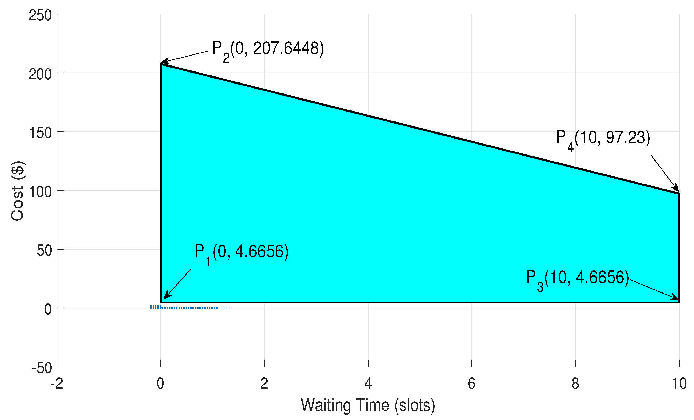
In our proposed scenario, the user discomfort is discussed in term of waiting time of devices. The maximum allowable waiting time for residential devices is 10 slots (i.e., 5 h). Figure 19 portrays the trade-off between the consumption cost and waiting time. User discomfort and electricity cost are inversely proportion to each other, by decreasing user discomfort electricity cost increases and vice versa. P1(0, 4.6656) and P2(0, 207.6448) show minimum and maximum consumption cost at zero waiting time. Consumers achieve maximum comfort at zero delay for the operational time of their devices. Whereas, P3(10, 4.6656) and P4(10, 97.23) denote minimum and maximum consumption at maximum waiting time.

6.7. Performance Trade-Off

It is deduced from the results that with the incorporation of user comfort in term of waiting time, the performance parameters are also affected. It can be viewed vividly from the same figure (i.e., GA and BPSO) that the user has achieved maximum monetary benefits, however, compromised on consumers’ convenience. Similarly, it is shown that GAPSO achieved comparatively less savings in electricity bills with maximum comfort level. In this way, electricity cost and user comfort both are efficiently addressed in the proposed model. The savings in electricity bills are decreased by 4.6779%, this decrement in savings is due to the fact that electricity cost and user comfort are inversely proportional to each other. By increasing the user comfort, savings in electricity bills are decreased and vice versa. The tradeoff between user comfort and cost is obvious since without sacrificing the convenience consumers are incapable of achieving the reduction in consumption cost.

In this work, we have considered uncontrolled parameters (without EMC) as bench mark; however, the results of the proposed technique are also compared with DP. The performance of the proposed approach is analyzed and is demonstrated in

Table 5. The Comparison of Performance Metrics for a Day.

Technique	Parameters	Lower Value	Upper Value
GA	Cost ($)	1106.7	1116.0
	Discomfort	0.1240	0.8941
	PAR	5.8204	6.1599
BPSO	Cost ($)	1201.4	1205.2
	Discomfort	0.2310	0.8421
	PAR	4.5706	4.7336
GAPSO	Cost ($)	1179.6	1182.8
	Discomfort	0.1102	0.8100
	PAR	4.4858	4.5283
DP	Cost ($)	1175.6	1175.6
	Discomfort	0.1102	0.8100
	PAR	4.2350	4.2315

. Table shows the upper and lower ranges of energy consumption cost, user discomfort and peak demand reduction. By analyzing the deviations between upper and lower values, it is deduced that the proposed model achieved the desired objective with 95% confidence interval. Moreover, optimality of the proposed model is also analyzed, as the DP provides optimal results. The difference between the performance parameters of proposed technique and that of DP provides the optimality gap.

Table 6. Monthly Energy Consumption Cost and Peak Load.

Technique	Parameters	Without EMC	With EMC	Reduction (%)
GA	Cost ($)	57,584	45,771	20.5143
	Peak-Load (kW)	41,088	32,136	21.7873
BPSO	Cost ($)	57,584	48,550.5	15.6883
	Peak-Load (kW)	41,088	26,928	34.4626
GAPSO	Cost ($)	57,584	43,765	23.9979
	Peak-Load (kW)	41,088	27,476	33.1288
DP	Cost ($)	57,584	43,840	23.8677
	Peak-Load (kW)	41,088	27,400	33.331

provides the monthly energy consumption cost and the peak load. It is clear from the figures provided in this table that as compared to GA and BPSO, GAPSO benefits the consumers by reducing their cost significantly. We have noticed that there is no significant difference between cost reduction by GAPSO and DP; however, we still prefer GAPSO over DP due to its computational efficiency which is clear from

Table 7. Computational Time of Employed Heuristic Techniques.

Techniques	Computation Time (Seconds)
GA	0.68
BPSO	0.59
GAPSO	0.55
DP	0.7

. The computational time of the proposed technique for 112 residential devices is also analyzed and compared with other considered techniques. Moreover, Table 7 portrays the time analysis of the proposed heuristic technique with DP, thus depicting the efficiency of the proposed technique with the deterministic approach in terms of computational time. The results clearly elucidate that our proposed technique; GAPSO solves the formulated problem with least amount of time.

7. Conclusions

In this paper, we have modelled a residential energy management system proposing a hybrid technique for residential load scheduling. The scheduling problem is formulated through MKP mainly focusing on achieving the objectives of minimizing the electricity cost and consumers’ discomfort. We analysed the performance of our proposed model under four different parameters: power consumption, electricity cost, PAR and user discomfort. Furthermore, the performance of the proposed technique is analysed and compared with GA, BPSO and DP. Results demonstrate that the performance of the proposed model is comparable to that of DP. However, the proposed model is efficient as it requires less computational time and storage. The proportional relation between performance parameters is calculated and shown with the help of feasible regions. Simulation results show that the proposed hybrid scheme, GAPSO, performed better in terms of cost and occupants’ discomfort minimization along with reduction of peak power consumption compared to its counterpart schemes GA and BPSO.