Modeling of HVDC System to Improve Estimation of Transient DC Current and Voltages for AC Line-to-Ground Fault—An Actual Case Study in Korea

Abstract

A new modeling method for high voltage direct current (HVDC) systems and associated controllers is presented for the power system simulator for engineering (PSS/E) simulation environment. The aim is to improve the estimation of the transient DC voltage and current in the event of an AC line-to-ground fault. The proposed method consists primary of three interconnected modules for (a) equation conversion; (b) control-mode selection; and (c) DC-line modeling. Simulation case studies were carried out using PSS/E and a power systems computer aided design/electromagnetic transients including DC (PSCAD/EMTDC) model of the Jeju–Haenam HVDC system in Korea. The simulation results are compared with actual operational data and the PSCAD/EMTDC simulation results for an HVDC system during single-phase and three-phase line-to-ground faults, respectively. These comparisons show that the proposed PSS/E modeling method results in the improved estimation of the dynamic variation in the DC voltage and current in the event of an AC network fault, with significant gains in computational efficiency, making it suitable for real-time analysis of HVDC systems.

1. Introduction

In recent years, high voltage direct current (HVDC) technology has attracted growing attention for power transmission between networks. The first commercial HVDC system was installed in Sweden in 1954; a total transmission line capacity of 191,000 MW is currently installed around the world across 172 HVDC system projects [1]. 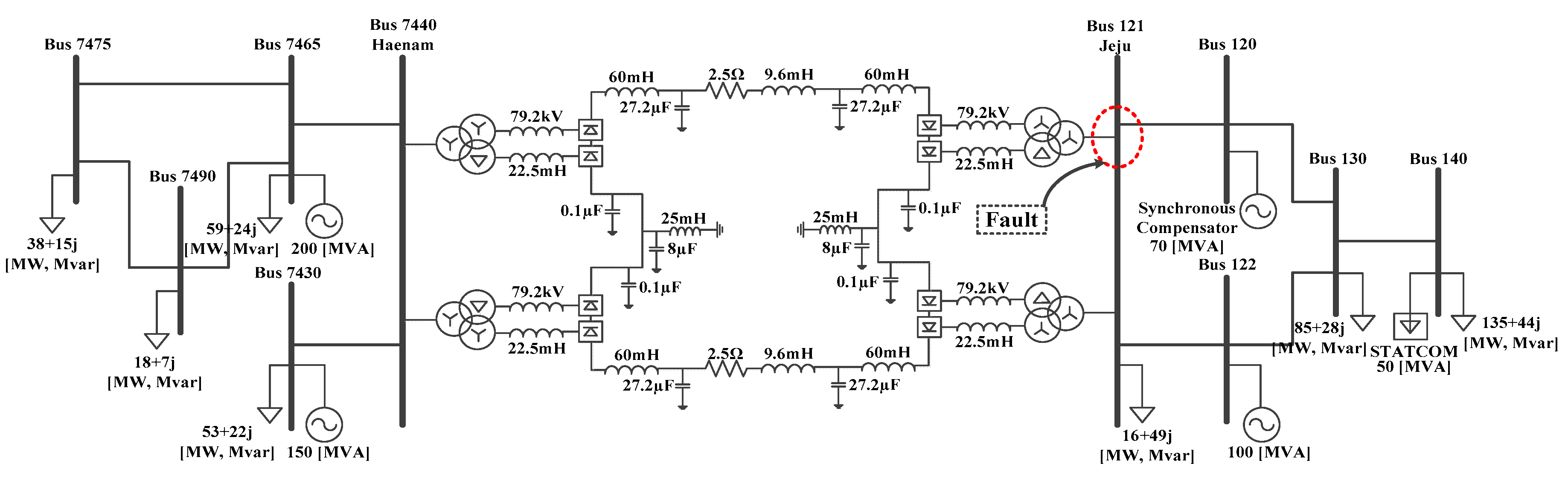Although voltage-source converters (VSCs) have been used in HVDC systems, line-commutated converter (LCC) schemes are also advantageous because they are a mature technology and are available at higher capacities for HVDC systems than current VSCs [2]. Based on these advantages, the 180-kV, 300-MW LCC–HVDC system installed by Korea Electric Power Corporation (KEPCO) has been used to convey relatively cheap electrical power from the Haenam substation on the Korean mainland to the Jeju substation on Jeju Island, via 100-km undersea cables [3].

Various models of HVDC systems have been developed to estimate operating conditions and analyze the transient and steady-state stabilities of LCC–HVDC systems and connected AC networks [4,5,6,7]. For example, in [4], the DC voltages and currents of LCC–HVDC systems were calculated in the common dq-reference frame of the associated AC network. Linearized models of LCC–HVDC systems were developed in [5,6] to analyze the dynamic power grid stability and the small-signal stability of multi-feed HVDC systems, respectively. In [7], the conseil international des grands reseaux electriques (CIGRE) benchmark HVDC system model was adopted to simulate a VSC-integrated LCC–HVDC system to connect an offshore wind farm to a mainland network. In [8,9], the operation of LCC–HVDC systems was investigated during commutation failure using the CIGRE benchmark model with respect to variations in the DC-line voltage and the valve current, respectively. However, the HVDC system models discussed so far need additional modifications to incorporate the operating characteristics of real HVDC systems because the parameters (e.g., rated power, voltage, etc.), controllers, and operations of some real HVDC systems often differ from those of the CIGRE benchmark. For example, the HVDC system in the Taiwan power grid was modeled in [10], where the CIGRE benchmark model was extended to include an extinction angle controller at the rectifier side, a DC current controller at the inverter side, and a voltage-dependent current order limit (VDCOL) function. The Anshun–Zhaoqing HVDC system model developed in [11] was not based on the CIGRE benchmark model, as the challenge of integrating it with the system operating characteristics was too difficult. Furthermore, the DC-lines in the above-mentioned system models were represented using a simple T-equivalent circuit, which has a limited accuracy for calculating variations in DC-line voltage and current. This inhibits direct application of the models and analyses to real systems, such as the Jeju–Haenam HVDC system (i.e., the KEPCO benchmark model).

Meanwhile, LCC–HVDC systems are susceptible to commutation failure on a weak AC grid or under AC line-to-ground fault conditions, which will interrupt the transmitted power and stress the converter equipment [12]. Therefore, there have been many studies on commutation failure recognition caused by the AC faults [13] and commutation failure mitigation by using the modified controllers [14,15] or by adding additional components/power electronic devices [16,17]. In [13], the method to calculate the maximum-allowable balanced voltage drop at an inverter AC busbar was proposed to determine the onset of commutation failures. The objectives of the modified controllers were either to reduce the probability of commutation failure or to increase the recovery speed of the DC system after commutation failure. One of the common methods is to advance the firing angle at the inverter side immediately after the detection of AC voltage disturbance in order to give a larger commutation margin [14]. Another method is to reduce the commutated DC current by decreasing the current order at the rectifier side upon detection of AC voltage disturbance [15]. Among the methods with additions of components/power electronic devices, capacitor-commutated converters (CCC) have been considered the most popular, as they can operate at a better power factor and have a lower probability of commutation failures [16]. In addition, the improved line-commutated converter with thyristor-based full-bridge module (TFBM), which is embedded in the converter valve, was proposed to enhance the commutation failure immunity in [17]. However, these papers discussed so far were concerned with the recognition or mitigation of commutation failure caused by AC line-to-ground fault. In the studies, the maximum DC current and voltage of the HVDC system have not been considered when commutation failures occur due to the AC line-to-ground fault. The maximum fault current and voltage are the primary concern for analyzing the transient stabilities of the AC network and HVDC system; for example, to determine the setting parameters of protection relays and the capacities of DC transmission lines and AC/DC converter valves [18,19,20].

In addition, several digital simulators have been adopted for simulation studies on LCC–HVDC systems. In particular, power systems computer aided design/electromagnetic transients including DC (PSCAD/EMTDC, or simply PSCAD) and Matlab/Simulink have been used to elaborate the control schemes of CIGRE HVDC benchmark system models [21,22,23]. However, the AC network models used in these studies were simplified by using voltage sources and equivalent impedances, primarily because of the models’ limited ability to model complex, large-scale AC networks. Therefore, real power grids—such as those on the Korean mainland and Jeju Island connected via the Jeju–Haenam HVDC system—are difficult to model using these simulators; i.e., real-time analysis of the HVDC systems will become computationally onerous.

The power system simulator for engineering (PSS/E) is a powerful time-domain simulator for the analysis of AC grids and associated controllers. It provides transmission planning and operation engineers with a broad range of methods for the design and operation of reliable networks. Many companies have therefore used PSS/E to analyze large-scale power grids. Moreover, PSS/E enables use of real AC grid data to describe interactions between an HVDC system and the AC power grid. There are also a few useful examples of HVDC models such as CDC4T, CDC6T, and CDC7T in PSS/E [24]. However, these models require large sets of parameters, which are typically difficult to obtain from real HVDC systems because of modeling discrepancies and confidentiality issues imposed by device manufacturers. Power grid operators and utility companies therefore require new PSS/E models for real-time analysis of practical HVDC systems; in designing such a model, we focused on the Jeju–Haenam HVDC system in Korea.

Based on the above observations, this paper describes a new modeling method for an HVDC system in the PSS/E simulation environment. The proposed method consists of three modules for (a) equation conversion; (b) control-mode selection; and (c) DC-line modeling, which are parameterized based on the unique characteristics of the Jeju–Haenam HVDC system and the Korea–Jeju power grid as a particular example. The results of the proposed model are compared with measured data for the actual HVDC system to demonstrate the effectiveness of the proposed modeling method. The main contributions of this paper are summarized as follows:

• The converting equations for abnormal operation, which particularly arise because of commutation failure under the conditions of fault occurrence in the AC transmission network, are developed and integrated into PSS/E to estimate the variations in the DC voltages and currents of the HVDC system.
• The HVDC system converters are equipped with feedback controllers. These enable us to easily determine the firing angles and obtain sufficiently accurate characteristic V-I curves, particularly with respect to the VDCOL function. Furthermore, the DC line is modeled using multiple π-sections for accurate estimation of the DC voltages and currents of the HVDC system.
• The proposed modeling method provides accurate estimates of the DC voltages and currents arising from AC line-to-ground faults. To the best of our knowledge, this paper is the first demonstration of an HVDC system model developed specifically with a quasi steady state (QSS)-type simulator using actual operating data from a real HVDC system for a single line-to-ground fault. The proposed model is also verified through comparisons with simulation results obtained from the comprehensive HVDC system model, developed using PSCAD, for the three-phase line-to-ground fault.
• The proposed method leads to a significant reduction in computational time. This will allow grid operators to perform efficient case studies of LCC-based HVDC systems under a variety of conditions. Furthermore, the proposed method can be implemented in coordination with commercial software, and independently of the built-in subsystems or algorithms for other dynamic power devices. It is easy to adapt the model to reflect the operating characteristics of specific HVDC systems without affecting the built-in functions. Hence, this model has a wide range of potential applications.

Section 2 explains the modeling justifications of the HVDC system in the PSS/E simulation environment. Section 3 presents the proposed modeling methods for an HVDC system based on the Jeju–Haenam HVDC system. Section 4 discusses the simulation case study results for both single-phase and three-phase line-to-ground faults at the inverter side. Section 5 provides our conclusions.

2. Modeling the HVDC System in the PSS/E Simulation Environment

An HVDC system can be modeled with various simulation time-steps depending on simulation tools such as PSCAD, Matlab/Simulink, and PSS/E. Specifically, PSCAD and Matlab/Simulink use 50-μs and 1-ms base simulation time-steps, respectively. These simulation tools are appropriate for developing a detailed model of an HVDC system, particularly at the valve- and firing-control levels. However, models of AC power transmission networks interconnected with HVDC systems require simplification. This is because the small time-steps in the simulation tools are inappropriate for dynamic analysis of large-scale transmission networks that include a number of loads, generators, and other components with non-linear operational characteristics. For example, in [25,26], valve-control methods for HVDC systems were proposed using these simulation tools; however, the test transmission networks were simply modeled using ideal voltage sources and equivalent Thevenin impedances.

The PSS/E software package is for simulating system phenomena at the fundamental frequency or below. PSS/E is thus appropriate for analyzing HVDC systems with respect to interaction with interconnected transmission networks. Measured data for a real transmission network can also be readily incorporated into PSS/E. Power flow calculation (PFC) is a PSS/E module that solves a set of algebraic equations to estimate the power outputs of generators and power flows in the network for a given load demand. Dynamic simulation (DS) is a module for calculating sets of differential equations, to analyze the electromagnetic transient operation of AC transmission networks [27]. Because of the relatively large simulation time-steps in PSS/E, HVDC system modeling scopes in PSS/E often include a constant current loop level, voltage-dependent current order limit (VDCOL), and master control. Furthermore, it normally takes only a few seconds to analyze the dynamics of an HVDC system, which is advantageous for both power grid operators and researchers.

In view of these benefits, the CIGRE HVDC benchmark system was recently modeled using PSS/E [28]. However, the CIGRE benchmark model needs to be modified when evaluating the transient-state operation of a real HVDC system triggered by transmission network events. The rated power and rated DC and AC voltages of a real HVDC system often differ significantly from those in the CIGRE HVDC system; for example, see

Table 1. Comparison between the Jeju–Haenam and CIGRE high voltage direct current (HVDC) system models.

Parameters	Jeju–Haenam HVDC	CIGRE HVDC
AC base voltage	Rectifier: 154 kV	Rectifier: 345 kV
	Inverter: 154 kV	Inverter: 230 kV
Nominal DC voltage	184 kV	500 kV
Nominal DC current	0.815 kA	2 kA
Source impedance (Rec)	R = 0.00675 Ω	R = 3.737 Ω
	L = 0.04653 H	L = 0 H
Source impedance (inv)	R = 0.00675 Ω	R = 0.7406 Ω
	L = 0.04653 H	L = 0.0365 H
System frequency	60 Hz	50 Hz
Converter control	Rectifier: voltage	Rectifier: current
	Inverter: current	Inverter: voltage

for the Jeju–Haenam HVDC system in Korea. In addition, the CIGRE benchmark only includes the DC current controller and extinction angle controller at the rectifier and inverter sides, respectively. Therefore, additional controllers are required to control the DC voltage at the rectifier side of the Jeju–Haenam HVDC system. Furthermore, the built-in VDCOL function provided in the CIGRE benchmark model only takes two set points, the pair (V_dc, I_dc), as input. This is often inconsistent with the operating characteristics of real HVDC systems; for example, the Jeju–Haenam HVDE system takes nine set points. Additionally, although there are sample models for HVDC systems in PSS/E, such as CDC4T, CDC6T, and CDC7T, they require 25, 35, and 79 system parameters, respectively. Furthermore, specific parameters representing the characteristics of an HVDC system must be implemented separately in PSS/E to analyze the transient-state operation of a real HVDC system accurately. For example, the sample models do not have a parameter for the gradual restoration of the DC voltage, as occurs during operation of the Jeju–Haenam HVDC system.

To use the PSS/E software to bridge the divide between academic research and practical applications, we therefore modeled a real HVDC system, the Jeju–Haenam HVDC system as a specific example, while considering fault events in the Jeju AC power grid.

3. Proposed Modeling Method for Improved Transient-State Analysis of HVDC Systems

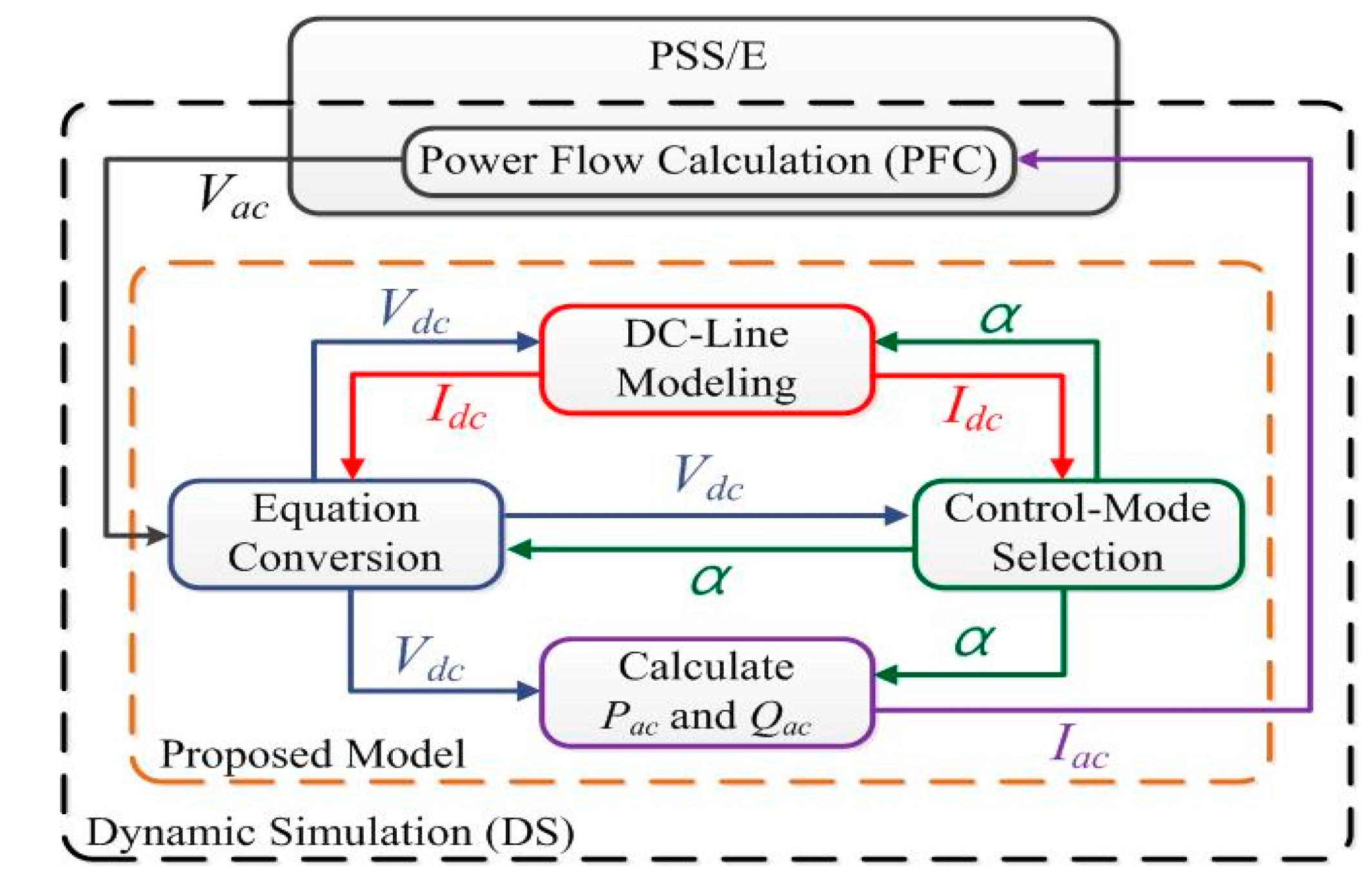
Figure 1 shows a schematic diagram of the proposed modeling method, which includes three modules for (a) equation conversion; (b) control-mode selection; and (c) DC-line modeling. The AC voltage V_ac on the primary side of the converter transformer is calculated using the PFC module of PSS/E. The DC-line current I_dc and converter firing angle α are obtained from the modules for DC-line modeling and control-mode selection, respectively. The DC-line voltage V_dc and other quantities associated with V_ac, I_dc and α are calculated in the equation conversion module. In the module for control-mode selection, α is then updated using the calculated V_dc and I_dc. The updated V_dc and α are used to update I_dc in the module for DC-line modeling. The converter output power P_ac and Q_ac are calculated using V_dc and α to provide the value of I_ac to PSS/E. PSS/E then updates V_ac using the updated I_ac in the PFC module. These calculations are performed iteratively as part of the DS process.

3.1. Equation Conversion

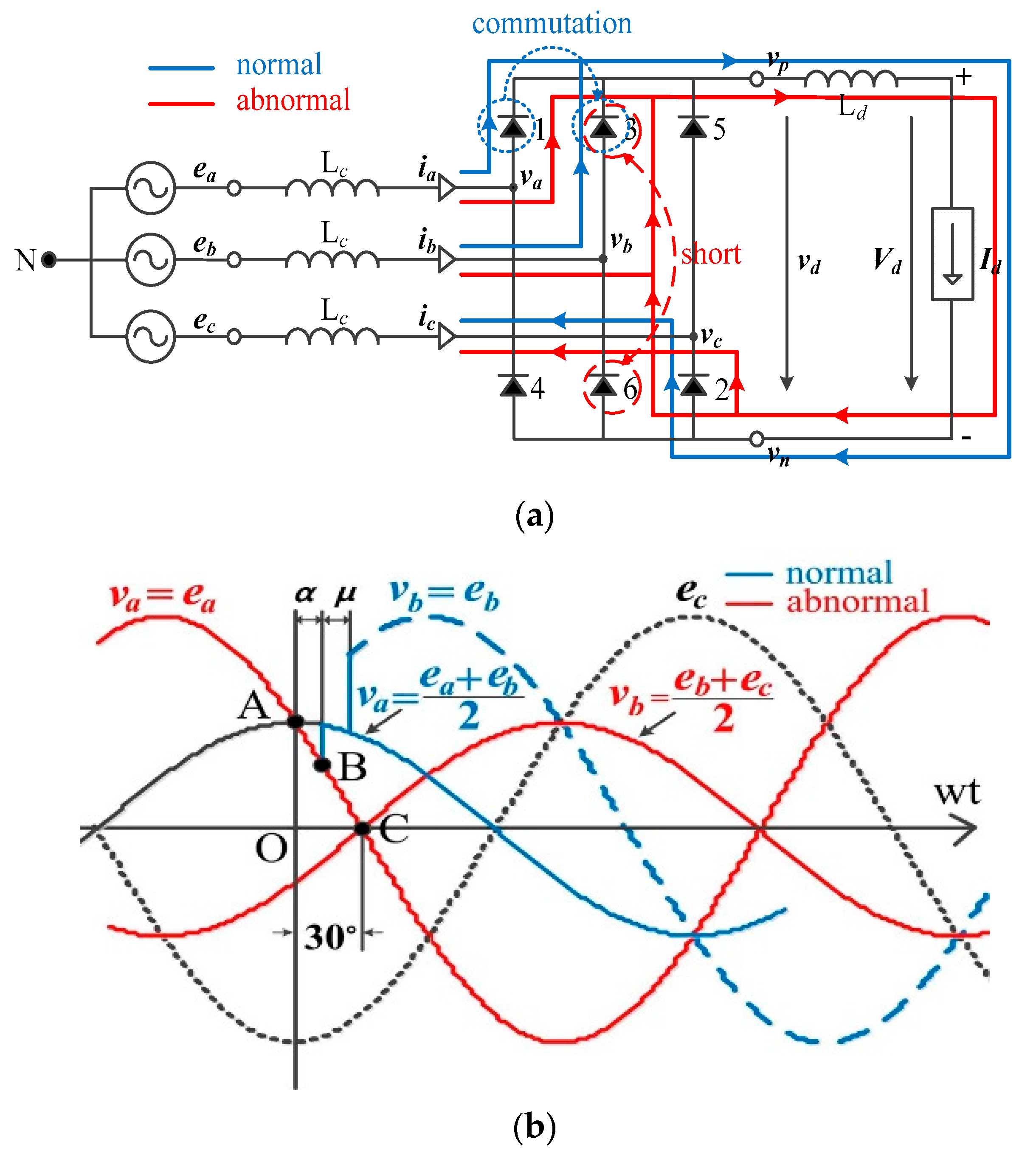
The main objective of the equation conversion module is to calculate the DC voltage of an HVDC system using I_dc and α, which are calculated by the DC-line modeling and the control-mode selection modules, respectively. The algebraic equations for P_ac and Q_ac, are then solved in the “calculate P_ac and Q_ac module” to calculate the I_ac, which is injected into the AC grid under normal and abnormal operating conditions. Under normal conditions, the overlap angle μ is less than 60° and two or three valves (i.e., Valves 1, 2, or 3) are conducted, as shown in Figure 2a. When a commutation occurs, the next valve is fired when its voltage exceeds the voltage of the valve currently operating; for example, Valve 3 will commutate from Valve 1 when v_b > v_a (i.e., the point A in Figure 2b). However, because of α, the next valve to be fired (i.e., Valve 3) will not conduct during time period α (i.e., the point B) and then the two Valves 1 and 3 on the upper side will conduct during the period μ, as shown in Figure 2b. Under abnormal conditions, μ is larger than 60° and four valves (i.e., Valves 1, 2, 3 and 6) are conducted. This results in a short circuit (i.e., the conducting of Valves 3 and 6), as shown in Figure 2a. v_a and v_b then become equal to e_a and (e_b + e_c)/2, respectively. Therefore, Valve 3 is ignited at the point C, where v_b > v_a under the abnormal condition.

The initial AC active and reactive powers of the HVDC converters are calculated from the AC voltage and current inputs; these values are calculated using the PFC module in PSS/E. Using the power flow calculation results, the DC voltage of the HVDC system is calculated using Equation (1), where α is obtained from the control-mode selection module. The overlap angle μ can also be calculated using the value of α in Equation (2). The active power P_ac and the power factor angle ϕ are then acquired using the updated values of V_dc, α, and μ, as shown in Equations (3) and (4), respectively. For the next iteration of the AC power flow calculation, the reactive power Q_ac is also obtained using Equation (5) such that the injected AC current to the HVDC converters can be calculated using Equations (3) and (5).

$$V_{dc}=N_c\left(\frac{3\sqrt{2}}{\pi }{E}_{acc}\cos \alpha -\frac{3X_{cc}{I}_{dc}}{\pi }-2R_{cc}{I}_{dc}\right)$$

(1)

$$\mu =\arccos \left(\cos \alpha -\frac{\sqrt{2}{I}_{dc}{X}_{cc}}{E_{acc}}\right)-\alpha$$

(2)

$$P_{ac}=\frac{3N_c{E}_{acc}^2}{4\pi X_{cc}}\left(\cos \left(2\alpha \right)-\cos 2\left(\mu +\alpha \right)\right)$$

(3)

$$\tan \left(\varphi \right)=\frac{2\mu +\sin \left(2\alpha \right)-\sin \left(2\left(\mu +\alpha \right)\right)}{\cos \left(2\alpha \right)-\cos \left(2\left(\mu +\alpha \right)\right)}$$

(4)

$$Q_{ac}=\frac{3N_c{E}_{acc}^2}{4\pi X_{cc}}\left(2\mu +\sin \left(2\alpha \right)-\sin \left(2\left(\mu +\alpha \right)\right)\right)$$

(5)

This paper focuses on the abnormal condition that arise in an HVDC system in the event of commutation failure; i.e., when the extinction angle γ falls below γ_min or where μ exceeds 60° [18,19,20,21]. If μ exceeds 60°, the subsequent commutation (i.e., from Valve 1 to Valve 3) will commence before completion of the current commutation (i.e., from Valve 2 to Valve 6). This results in a short circuit (i.e., the conducting of Valves 3 and 6), as shown in Figure 2a. v_a and v_b then become equal to e_a and (e_b + e_c)/2, respectively, as shown in Figure 2b. Valve 3 is ignited at the point C, where v_b > v_a under the abnormal condition, whereas it is fired at the point B due to α under the normal operation, as shown in Figure 2b. Thus, the DC voltage and current will be modified under the abnormal condition, as seen in Equations (6) and (7).

$$V_{dc}=N_c\left(\frac{3\sqrt{6}}{2\pi }{E}_{acc}\left(\cos \left(\alpha -30\right)+\cos \left(\delta +30\right)\right)\right)$$

(6)

$$I_{dc}=\frac{1}{\sqrt{6}\left(X_{cc}+\raisebox{1ex}{$2\pi $}\!\left/ \!\raisebox{-1ex}{$9$}\right.R_{cc}\right)}{E}_{acc}\left(\cos \left(\alpha -30\right)-\cos \left(\delta +30\right)\right)$$

(7)

By substituting Equation (7) into Equation (6), V_dc can be represented as (8). Furthermore, γ and Equations (3)–(5) are accordingly modified under the abnormal condition to Equations (8)–(12). These equations are not reflected in the conventional sample models (i.e., CDC4T, CDC6T, and CDC7T) in PSS/E. Therefore, the proposed modeling method improves estimation of the DC voltage, DC current, and AC current that is injected into the converters during the transient operation of the HVDC system triggered by commutation failure.

$$V_{dc}=N_c\left(\frac{3\sqrt{6}}{\pi }{E}_{acc}\cos \left(\alpha -30\right)-\frac{9X_{cc}{I}_{dc}}{\pi }-2R_{cc}{I}_{dc}\right)$$

(8)

$$\gamma =\arccos \left(\cos \left(\alpha -30\right)-\frac{\sqrt{6}{I}_{dc}{X}_{cc}}{E_{acc}}\right)-30$$

(9)

$$\tan \left(\varphi \right)=\frac{2\mu +\sin \left(2\left(\alpha -30\right)\right)-\sin \left(2\left(\gamma +\alpha \right)\right)}{\cos \left(2\left(\alpha -30\right)\right)-\cos \left(2\left(\gamma +30\right)\right)}$$

(10)

$$P_{ac}=\frac{3N_c{E}_{acc}^2}{4\pi X_{cc}}\left(\cos \left(2\left(\alpha -30\right)\right)-\cos 2\left(\gamma +30\right)\right)$$

(11)

$$Q_{ac}=\frac{3N_c{E}_{acc}^2}{4\pi X_{cc}}\left(2\mu +\sin \left(2\left(\alpha -30\right)\right)-\sin \left(2\left(\gamma +30\right)\right)\right)$$

(12)

3.2. Control-Mode Selection

The module for control-mode selection calculates α for the rectifier and the inverter. The control mode of HVDC converters can be changed from current control to voltage control, and vice versa, according to the AC voltage conditions at the converter output ports. Many HVDC system device manufacturers (e.g., ABB, SIEMENS, and ALSTOM) have developed methods for selecting the control mode. For example, ABB implements control mode selection by changing the minimum or maximum limits of the DC current controllers [29]. In their system, DC voltage control is executed first, and the output of the DC voltage controller is set to the minimum or maximum limits of the DC current controller on both sides [28]. However, different HVDC systems may have differing V-I characteristics, which makes implementation difficult using either the CIGRE benchmark model or the proprietary control models developed by particular manufacturers. Therefore, in this paper, a rather simple and straightforward HVDC controller is proposed to facilitate analysis of dynamic variations in DC-line voltages and currents. With some minor modifications, the proposed controller is easily applicable to other types of HVDC systems; e.g., KEPCO has used a controller to model the Jeju–Jindo HVDC system [30].

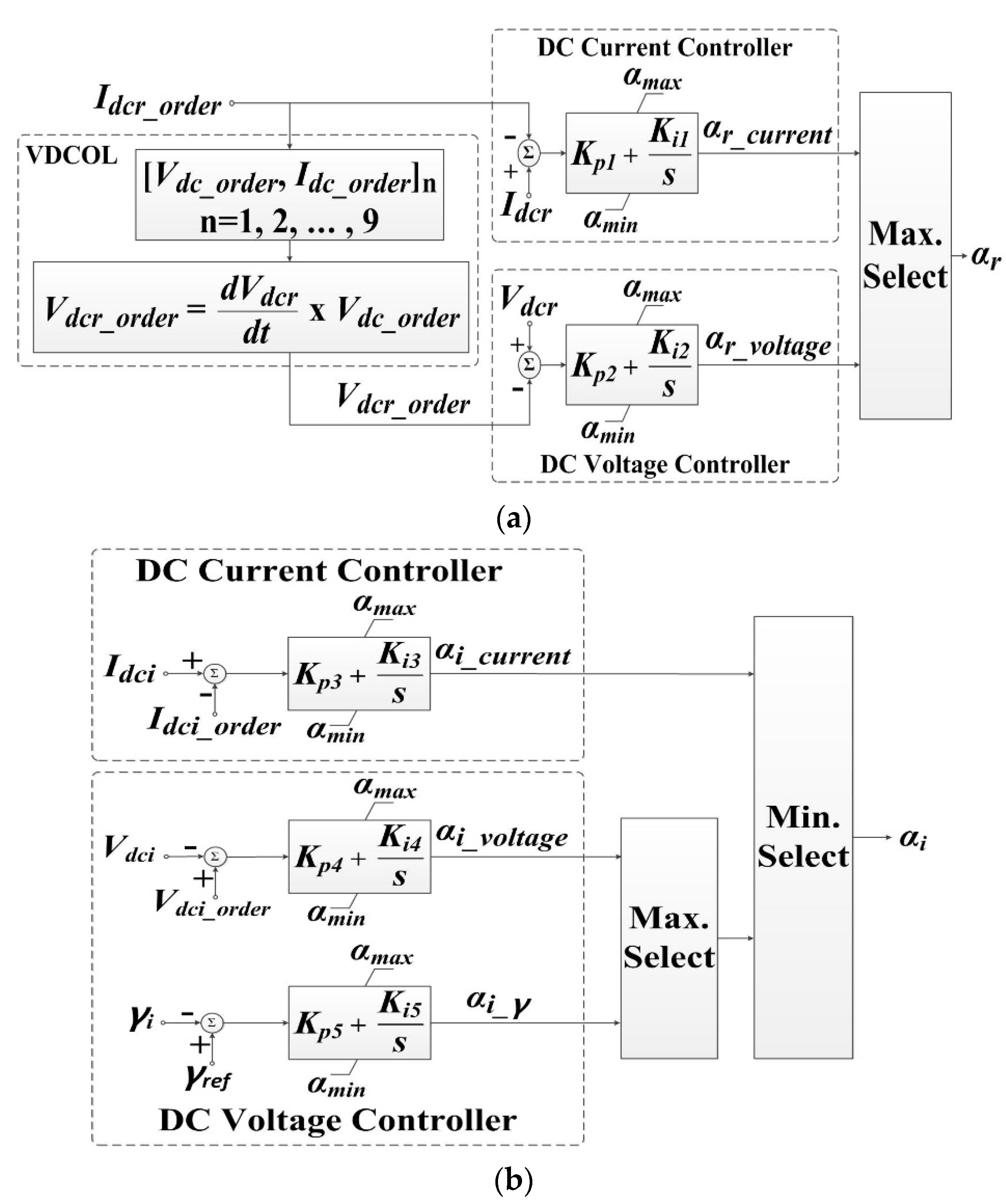
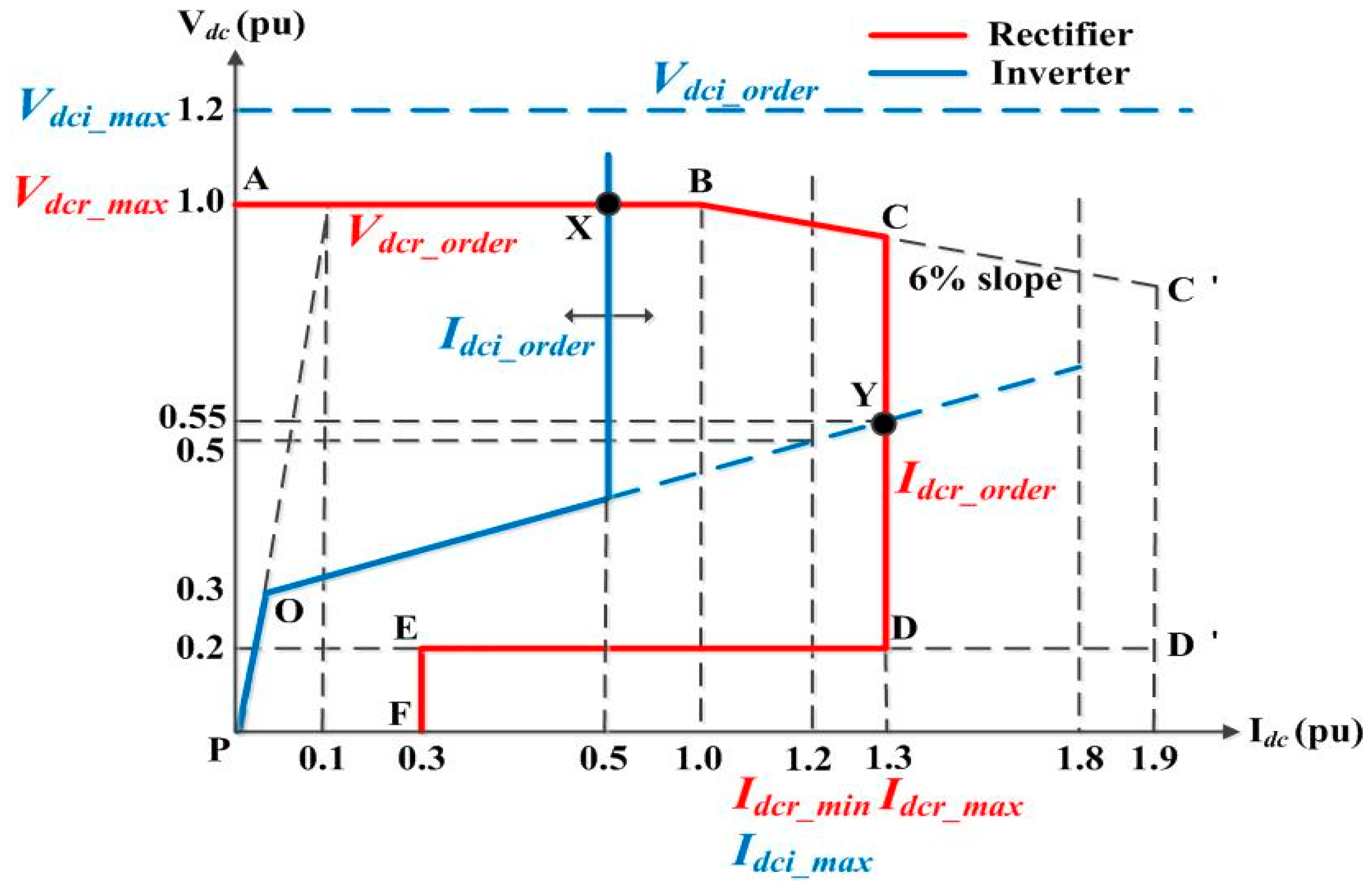
Figure 3 shows a simplified schematic diagram of the proposed scheme for control-mode selection for the rectifier and inverter of the Jeju–Haenam HVDC system, which has a V-I characteristic curve as shown in Figure 4. In the proposed scheme, the control mode to achieve the smallest difference between the reference and current values of the DC voltage and current is determined. For the rectifier, there are two proportional integral (PI) controllers with pre-determined maximum and minimum output limitations. If the rectifier controls the DC voltage under the normal operations (i.e., the point X in Figure 4), then the DC voltage and current of the rectifier become very close to V_dcr = 1.0 pu and I_dcr = 0.5 pu. The reference DC voltage and current at the rectifier side are V_{dcr_order} = 1.0 pu and I_{dcr_order} = 1.3 pu, as shown in Figure 4. Therefore, the difference between V_{dcr_order} and V_dcr is so small that the output signal α_{r_voltage} of the DC voltage controller at the rectifier is close to the current rectifier firing angle α_r, which is normally within the range from 15° to 20°. On the other hand, the DC current controller decreases the output signal α_{r_current} so as to increase I_dcr up to I_{dcr_order}. This is because I_dcr is calculated using the difference between V_dcr, which is proportional to cos α_r, and the DC voltage at the middle of the DC line. In other words, a decrease in α_r is equivalent to an increase in I_dcr by increasing V_dcr. Therefore, α_{r_current} is smaller than α_{r_voltage}, which is chosen as an updated α_r using the maximum selection function.

Furthermore, the rectifier controls the DC current when the AC network voltage drops (i.e., the point Y in Figure 4). The voltage and current become very close to V_dcr = 0.55 pu and I_dcr = 1.3 pu. V_{dcr_order} and I_{dcr_order} are similar, as discussed above (1.0 and 1.3 pu, respectively). Thus, the DC voltage controller decreases α_{r_voltage} so as to increase V_dcr up to V_{dcr_order}. However, α_{r_current} is close to current α_r due to the small difference between I_{dcr_order} and I_dcr. Consequently, the updated α_r is chosen from the DC current controller. α_min is normally larger than 5° to ensure adequate voltage across the valve before firing and α_max is normally between 90° and 170° to operate in the inverter region to assist the system under certain fault conditions.

The control-mode selection of the inverter side is similar to that at the rectifier side, apart from the additional PI controller for γ selection as shown in Figure 3b. Under normal operation (i.e., point X in Figure 4), the inverter DC voltage and current become very close to V_dci = 1.0 pu and I_dci = 0.5 pu. The reference DC voltage and current at the inverter side are V_{dci_order} = 1.2 pu and I_{dci_order} = 0.5 pu. Thus, the difference between I_{dci_order} and I_dcr is so small that the output signal α_{i_current} of the DC current controller at the inverter is close to the current inverter firing angle α_i. However, the DC voltage controller increases the output signal α_{i_voltage} so as to increase V_dci up to V_{dci_order}; V_dci is proportional to cos (π – α_i). Therefore, α_{i_voltage} is larger than α_{i_current}, which is chosen as an updated α_i using the minimum selection function.

Analogously, when the inverter controls the DC voltage (i.e., the point Y in Figure 4), α_{i_current} is increased so as to decrease the DC current from I_dci = 1.3 pu to I_{dci_order} = 0.5 pu. This is because I_dci is calculated using the difference between the DC voltage at the middle of the DC line and V_dci. In other words, an increase in α_i means a decrease in I_dci by increasing V_dci. On the other hand, α_{i_voltage} is similar to the current α_i due to the small difference between V_dci and V_{dci_order} of 0.55 pu. Therefore, the updated α_i is chosen from the DC voltage controller. The γ controller is an auxiliary controller and is not discussed further for brevity.

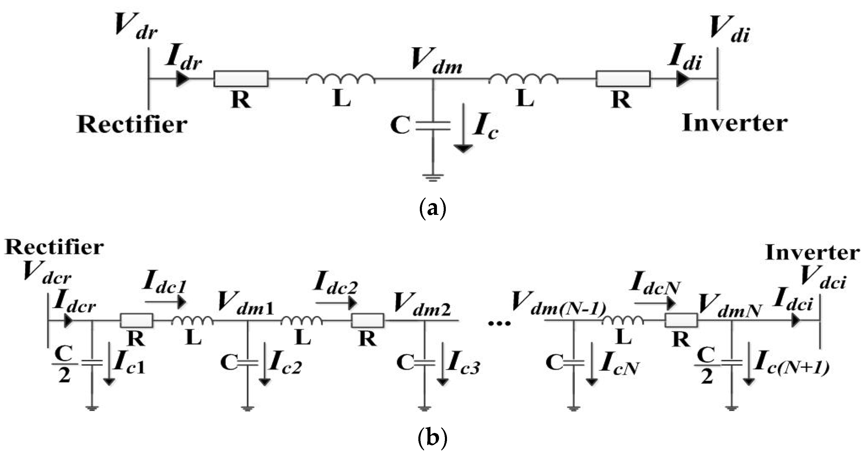
3.3. DC-Line Modeling

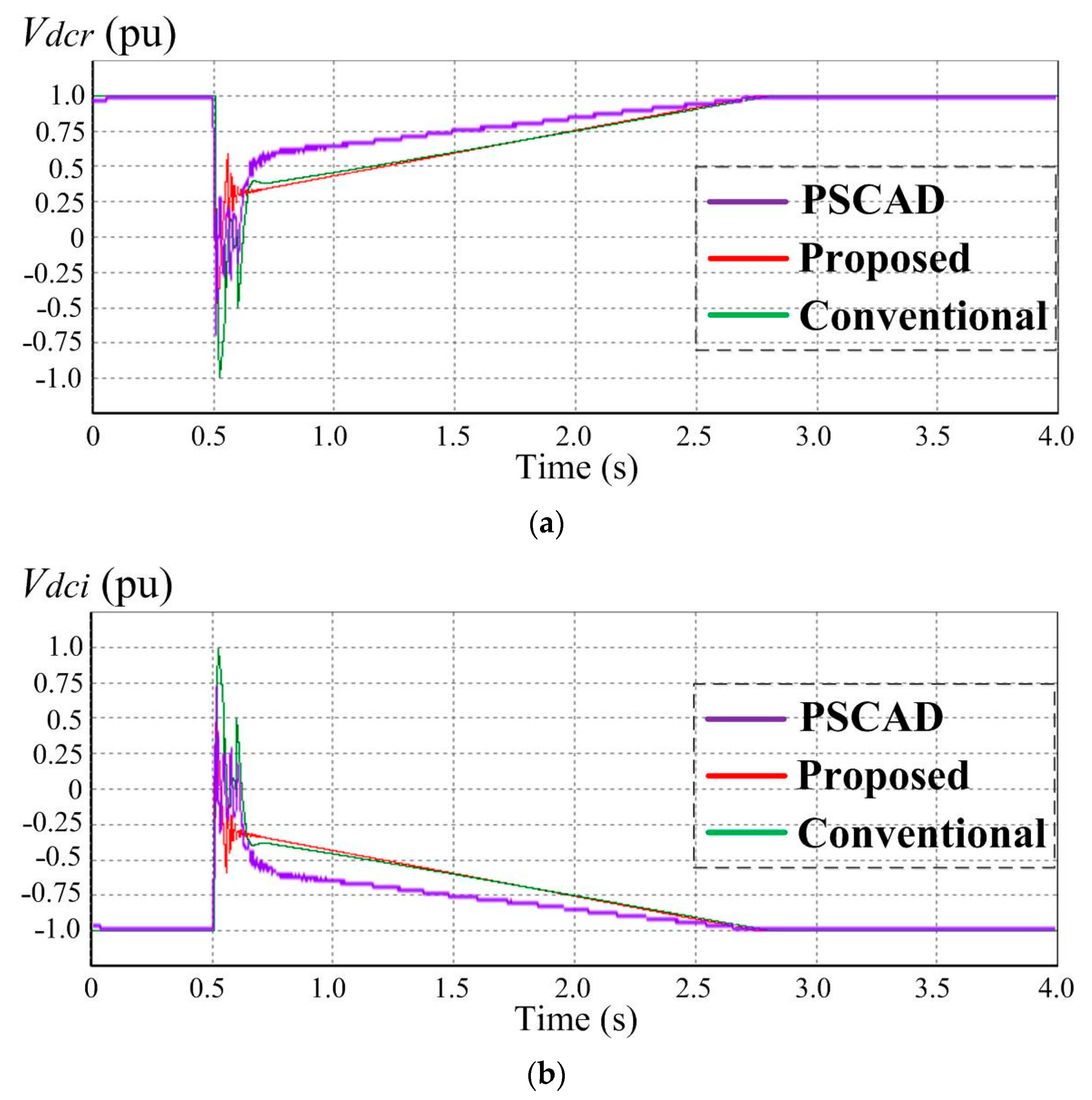
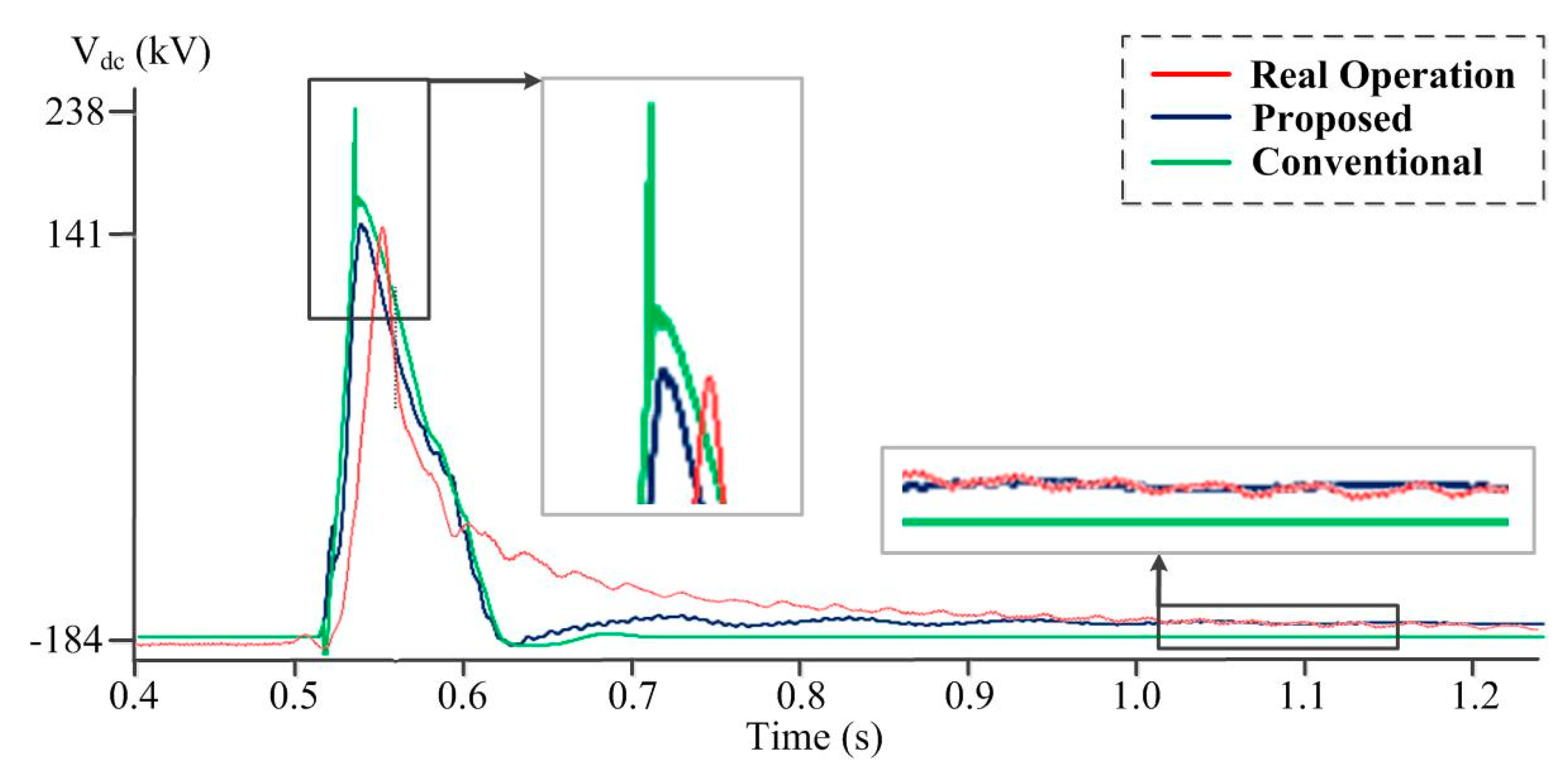
In the DC-line modeling module, the DC currents at the rectifier and inverter are calculated using the updated DC voltages (i.e., Equations (1) and (8)) under the normal and abnormal operating conditions, respectively, as well as α at each simulation time-step. Figure 5 shows a comparison between the conventional and proposed DC-line models. In [31], the DC line of the HVDC system was modeled using a π-section. The accuracy of the estimation increases with the number of π-sections used, as discussed in Section 4.

The conventional DC-line model has been used in many previous papers [7], references [32,33] because of its simplicity. However, it may overestimate the fault current, particularly with PSS/E, when there is a commutation failure resulting from a single-phase or three-phase line-to-ground fault in the AC network. Specifically, in the conventional DC-line model, the fault current mainly arises from the difference between the DC voltages V_dm at the middle of the DC line and V_dci at the inverter side. In the proposed model, the fault current mainly arises from the difference between V_dm(n-1) and V_dmn, as shown in Figure 5b. Note that V_dm0 and V_dmN are equal to V_dcr and V_dci, respectively. The difference between V_dm(n-1) and V_dmn may approximate the actual fault more accurately than the difference between V_dm and V_dci. This is because the actual DC-line has a uniformly distributed resistance R, inductance L, and capacitance C. The DC voltage and hence current are influenced by the line components punctuated in the DC-line.

However, as the number of differential equations required to calculate I_dci increase with the number of π-sections, it becomes more difficult to evaluate the PI gains (e.g., K_p3 and K_i3 in Figure 3) of the rectifier and inverter controllers. Therefore, in this paper, we settled the trade-off between the modeling accuracy and computational complexity by using three π-section lines (i.e., N = 3) to model the DC line.

4. Simulation Case Studies and Results

4.1. Test System and Simulation Conditions

Figure 6 shows a simplified schematic diagram of the test grid. Note that the test grid is the entire AC network of Korea including the mainland and Jeju Island; the corresponding PSS/E data were used for simulation case studies. KEPCO acquired the PSS/E data for the transmission network model in 2015: it includes 382 generators, 1275 loads, and 1834 buses. The PSS/E model also includes data related to wind turbines, switched shunt capacitors, synchronous condensers (SCs), and static synchronous compensators (STATCOMs). The PSS/E model for Korean transmission networks has been comprehensively discussed in [34]. The detailed parameters of the Jeju–Haenam HVDC system are summarized in

Table 2. Detailed parameters of the Jeju–Haenam HVDC system.

	Parameter	Value	Parameter	Value
Input parameters for PSS/E	Prated (MW)	75	Vrated (kV)	184
	Nc	2	R	0.744
	Xcc	7.99	L	133.33
	Rcc	0	C	27
Parameters for proposed model	Vdcr_max (pu)	1	Vdci_max (pu)	1.2
	Idcr_min (pu)	1.2	Idcr_max (pu)	1.3
	Idci_max (pu)	1.2	αmax (°)	165
	αmin (°)	5	γref (°)	18
	Kp1	0.01	Ki1	0.001
	Kp2	1.3	Ki2	2.5
	Kp3	1.42	Ki3	5.5
	Kp4	0.01	Ki4	0.01
	Kp5	0.1	Ki5	0.01

. All the parameters in Table 2 were obtained considering the unique characteristics of the real Jeju–Haenam HVDC system [35]. Note that the Jeju–Haenam HVDC system is one of the benchmark models, which has different characteristics compared to the CIGRE benchmark system.

The proposed method for modeling an HVDC system was tested for the specific case when a transient AC-line fault occurs in a weak AC network. This is because AC single line-to-ground faults are the most frequent fault events in power grid operation [36] and occur regularly at HVDC stations or generator buses. Moreover, various problems (i.e., high dynamic over-voltages, voltage instability, and harmonic resonance) may occur when HVDC systems are connected to weak AC networks [37]. The AC network on Jeju Island is a weak grid with a short circuit ratio (SCR) of 4.0 [38]. Therefore, the response of the HVDC system to AC line faults at the inverter side (i.e., bus 121 in Figure 6) was investigated.

Simulation results obtained from the proposed HVDC model were compared with operating data from the Jeju–Haenam HVDC system at KEPCO using a comprehensive PSCAD model of the HVDC system. Detailed explanations of the PSCAD model can be found in [38]. For comparison with the real operational data, a single line-to-ground fault that occurred at the inverter side of the HVDC system model at t = 0.5 s for 0.015 s was considered. For comparison with PSCAD simulation data, it was assumed that a three-phase line-to-ground fault occurred at the inverter side at t = 0.5 s for 0.1 s. Note that the HVDC system was comprehensively modeled using PSCAD for the simulation case studies because there are no real operational data for three-phase line-to-ground faults in the Jeju transmission networks. In the PSCAD model, the HVDC system is connected with large-scale transmission networks on the Korean mainland and Jeju Island. The simulations were performed on a computer having the four-core CPU of 3.5 GHz and 16 G RAM.

4.2. Case Study A: Comparision with Real HVDC System

Figure 7 and Figure 8 show the DC voltage and current, respectively, at the inverter side when a single-phase line-to-ground fault occurred in the Jeju power network. The red line in Figure 7 shows the actual operational DC voltage at the inverter side when there was an A-phase fault at the Jeju station on 6 February 2015. When the fault occurred, the DC voltage increased rapidly to 141 kV after a small time delay, mainly because of a smoothing reactor on the DC-line, and then slowly decreased to the rated voltage. Similarly, the DC voltage of the proposed HVDC system model increased to 145 kV after the fault occurred, which is similar to the peak value in the real data. The proposed model recovered the DC-line voltage faster, particularly after t = 0.6 s, than the real HVDC system. This is because it is assumed in the PSS/E model that the valve or firing control is not implemented but is calculated using Equation (2) or (9), and the tap changer of the converter transformer has no time delay in the PSS/E model. In the conventional model, the DC voltage increased to 238 kV after the fault, although it showed similar transient behaviors, particularly during the time period of voltage increase and recovery. However, the proposed model improved the estimation of the DC voltage by calculating Equation (8), instead of Equation (1), when the single-phase fault occurred. In addition, the proposed model resulted in almost identical steady-state voltage to that of the real HVDC system after the fault, whereas the conventional model caused a noticeable discrepancy in the voltage.

Figure 8 shows a comparison of the DC currents at the inverter side in the proposed and conventional HVDC models. For the proposed HVDC model, the DC current increased to 2375 A; note that the maximum fault current for the real HVDC system was 2380 A. However, for the conventional model, the DC current increased to 3120 A, mainly because the voltage difference between V_dm and V_di in Figure 5a was larger than the difference between V_dm2 and V_di in Figure 5b. The maximum fault current is the primary concern for transient stability analysis of AC transmission network operation, for example, in the design of protecting relays, transmission line capacities, and converter valves [18,19]. Therefore, the proposed model can be effectively used for contingency analysis of transmission networks connected to HVDC systems.

4.3. Case Study B: Comparision with the PSCAD Model

Figure 9, Figure 10 and Figure 11 show the DC-line voltage and current at the inverter side when a three-phase line-to-ground short-circuit fault occurred in the transmission line at t = 0.5 s and was cleared at t = 0.6 s. As shown in Figure 9a,b, the PSCAD model and the proposed PSS/E model both resulted in similar values of the maximum (or minimum) DC voltage during the fault, whereas the conventional model resulted in larger peak values, as summarized in

Table 3. Comparisons of the peak values of the DC voltages for the three-phase line-to-ground fault.

DC Voltages	PSCAD		Proposed PSS/E		Conventional PSS/E
	Value	Error (%)	Value	Error (%)	Value	Error (%)
min. Vdcr (kV)	−126.4	-	−121.1	4.2	−180.5	42.8
max. Vdci (kV)	129.9	-	127.5	1.9	186.4	43.5

. This was mainly because of the equation conversion module considering the abnormal operation in the proposed method. In practice, the HVDC system controllers are designed to restore the DC voltage gradually (around 0.2 pu/s) to protect the weak transmission networks on Jeju Island. This is reflected in the proposed HVDC system controller, as discussed in Section 3.2, so that the DC voltage increases gradually to the rated voltage following a fault (i.e., during 0.6 < t < 2.7 s). Note that the maximum DC voltage between the rectifier and the inverter sides is mainly considered in this paper because it is used for calculating the maximum fault current and consequently designing protective relays, transmission line capacities, and converter values [18,19].

Figure 10a–c show the DC currents at the rectifier side for the PSCAD model, the proposed model and conventional PSS/E model. The PSCAD model and the proposed PSS/E model both exhibited similar peak currents of approximately 3.5 pu, whereas the conventional PSS/E model resulted in a larger peak of 3.9 pu. Analogously, as shown in Figure 11a–c, the DC current at the inverter side using the PSCAD model and the proposed PSS/E model were approximately 3.6 pu, whereas it was higher than 4.0 pu using the conventional PSS/E model. The DC current is estimated more accurately in the proposed PSS/E model, mainly because of the DC-line modeling method, as discussed in Section 3.3. The DC current increases more at the inverter side than at the rectifier side in all cases, because the difference between V_dm2 (or V_dm) and V_di was greater than V_dr and V_dm1 (or V_dm). Note that the minimum DC current was zero because the thyristor valves conduct only in one direction, which means that the DC current cannot be reversed [37,39].

Table 4. Summary of the maximum DC voltages and currents for the different DC-line models.

Key Quantities	Real Data	Proposed PSS/E Model, Error (%)
		3 π-Sections		2 π-Sections		1 π-Section		T-Line
		Value	Error	Value	Error	Value	Error	Value	Error
max. Vdci (kA)	141	145	2.8	161	14.1	198	40.4	238	68.8
max. Idci (A)	2380	2375	0.2	2643	11.1	2881	21.4	3120	31.1

lists the maximum DC voltage and current arising from a single line-to-ground fault at the inverter side, according to four different DC-line models and real operating data. The difference between the real data and the simulation results decreases as the number of π-sections increases.

The computation times required to simulate 4 s using the proposed and conventional models using PSS/E and PSCAD models are compared in

Table 5. Computation Time for 4-s Simulation Run.

Models	Proposed (PSS/E)	Conventional (PSS/E)	PSCAD
Time (s)	25	24	1276

. Both of the PSS/E models were significantly more time-efficient than the PSCAD model. The conventional model is slightly more time-efficient than the proposed model, but not significantly so. This is because the proposed model uses more differential equations in the π-section model of the DC line.

5. Conclusions

In this paper, a new modeling method for an HVDC system and associated controllers was proposed to improve the estimation of transient variations in the DC voltage and current when an AC line-to-ground fault occurs in an adjacent transmission network. In particular, the proposed method was developed considering incorporation into a commercial PSS/E simulator, which is more time-efficient for large-scale network simulation than a PSCAD simulator. The modeling method consists mainly of three modules for (a) equation conversion; (b) control-mode selection; and (c) DC-line modeling. Simulation case studies were then performed using the real operational data and the comprehensive PSCAD model of the Jeju–Haenam HVDC system in Korea (i.e., the KEPCO benchmark model) as an example. The case study results showed that the proposed modeling method is time-efficient and estimate the DC voltage and current variation more accurately for single-phase and three-phase line-to-ground faults when the HVDC system is modeled using the PSS/E simulator. According to the simulation results, the main contributions can be summarized as follows:

• The converting equations for abnormal operation, which particularly arises because of commutation failure under the conditions of fault occurrence in the AC transmission network, are developed and integrated into PSS/E to estimate the variations in the DC voltages and currents of the HVDC system accurately. Furthermore, the DC line is modeled using multiple π-sections for accurate estimation of the DC voltages and currents of the HVDC system considering the trade-off between the modeling accuracy and computational complexity. The simulation results show that the proposed modeling method, which includes the converting equations for abnormal operation and the π-section model of DC line, estimate the more accurate DC voltage and current variation than the conventional methods for single-phase and three-phase line-to-ground faults in PSS/E environment.
• To the best of our knowledge, this paper is the first in which an HVDC system model developed particularly in the PSS/E simulator is demonstrated using the actual operating data of a real HVDC system (i.e., the KEPCO benchmark model) for a single line-to-ground fault. The proposed model is also verified via comparisons with simulation results obtained from the comprehensive HVDC system model, developed using PSCAD, for the three-phase line-to-ground fault.
• The proposed method leads to a significant reduction in computational time, which allows grid operators to perform efficient case studies on LCC-based HVDC systems under a variety of conditions. In addition, the proposed method can be implemented in conjunction with commercial software and independently from the built-in subsystems or algorithms used to model other dynamic power devices. It is also easy to modify the models to reflect the operating characteristics of specific HVDC systems without affecting the built-in functions Therefore, the proposed modeling method enables grid operators in other countries to effectively perform similar case studies considering various size, types, and modeling complexities of LCC-based HVDC systems with some minor modifications.