Article

An Improved Forecasting Method for Photovoltaic Power Based on Adaptive BP Neural Network with a Scrolling Time Window

1
State Key Laboratory of Alternate Electrical Power System with Renewable Energy Sources, North China Electric Power University, Changping District, Beijing 102206, China
2
School of Renewable Energy, North China Electric Power University, Changping District, Beijing 102206, China
3
Beijing Key Laboratory of New and Renewable Energy, North China Electric Power University, Changping District, Beijing 102206, China
*
Author to whom correspondence should be addressed.
Energies 2017, 10(10), 1542; https://doi.org/10.3390/en10101542
Submission received: 25 August 2017 / Revised: 11 September 2017 / Accepted: 1 October 2017 / Published: 6 October 2017

Abstract

:
Due to the large scale of grid-connected photovoltaic (PV) power generation installations, accurate PV power forecasting is critical to the safe and economic operation of the electric power system. In the paper, by analyzing the influence of external ambient factors and the changing characteristics of PV modules with time, it is found that PV power generation is a nonlinear and time-varying process. This suggests that a certain single forecasting model is inadequate for representing actual generation characteristics, and it is difficult to obtain an accurate forecasting result. An adaptive back propagation (BP) neural network model adopting scrolling time window is proposed to solve the problem. Via an update of the training data of BP neural network with the scrolling time window, the forecasting model adapts to time and a changing external environment with the required modeling precision. Meanwhile, through evaluation of the forecasting performance in different time windows, an optimized time window can be determined to guarantee accuracy. Finally, using the actual operation data of a PV plant in Beijing, the approach is validated as being applicable for PV power forecasting and is able to effectively respond to the dynamic change of the PV power generation process. This improves the forecasting accuracy and also reduces computation complexity as compared with the conventional BP neural network algorithm.

1. Introduction

As energy and environmental issues become increasingly prominent, the effective and efficient utilization of renewable energy sources is a global challenge [1]. Photovoltaic (PV) power generation, the most promising type of solar energy utilization, has been developed surprisingly quickly, and plays an important role in the energy mix [2]. Considering the random fluctuation of solar energy resources, the access to grid-connected PV power generation relies on accurate and reliable power forecasting for the safety, stability, and economical operation of electric power system [3]. PV power forecasting can be performed using physical methods or statistical methods [4]. However, the modeling process of physical methods is complex, and the results may not be applicable for some extreme cases. For this reason, statistical methods have gradually become the most widely used forecasting method [5]. The statistical method mines substantial historical data to determine the inherent law of PV output generation and various determinants, and then builds a power forecasting model for the future output power of the PV plant [6]. Common statistical methods include support vector machine [7], and Markov chain [8], and artificial neural network [9], etc.
Because neural networks (NNs) have a strong nonlinear approximation ability and good generalization ability, they are widely applied in PV power forecasting [10]. The neural network forecasting model can be improved through the following three aspects, building a combined model with other advanced algorithms [11], optimizing input neuronal structure [12], and improving the internal network algorithm [13]. However, due to the influence of various factors, PV power generation is a nonlinear and time-varying process which includes the generation characteristic determined by the changing external environment and the degradation characteristic of PV modules. Although such complex nonlinear relationships can be represented by the neural networks to an extent, their dynamics are inadequate for representing the actual PV power generation characteristic when they are directly utilized [14]. Thus, in order to make it more suitable for artificial neural networks to be used in PV power forecasting, these data-driven algorithms should be further improved. According to the current literature, several aspects have been paid great attention for improving the PV power forecasting performance based on the artificial neural network. Firstly, for most PV power forecasting models in use, offline training is adopted, and the trained models remain unchanged when it is used. In comparison, online training is effective for the improvement of the forecasting model’s performance. Considering the dynamic characteristics of the PV power generation process, the accuracy of an offline trained neural network forecasting method is not ideal [15]. Ferlito et al. [16] proposed two different training methodologies (online and offline) to identify the most performing training mode. The “offline” mode carries out the training phase with the annual dataset. The “online” mode carries out the training process with the limited dataset. The analysis results show that a poorer forecasting accuracy was obtained in the “offline” training mode. Secondly, the use of adaptive models is another way to improve the accuracy. Considering the uncertainty of PV power, Li et al. [17] proposed a time-scale adaptive dispatch method for renewable energy power supply systems on islands. Eleonora et al. [18] proposed a scheduling approach for optimal dispatch of the electrical energy storage system. The approach is based on fuzzy rules which self-adapt their membership functions using an economic indicator. Dash et al. [19] demonstrated a real-life application to forecast the real power output of a PV system connected to a local load by using intelligent tools, which primarily comprised dynamic neural networks which are capable of time-series predictions with good reliability. Thirdly, the hybrid method is also a good solution to problems. Liu et al. [20] shows that it is feasible to design a simple, satisfactory forecasting model based on fuzzy logic and neural networks to predict very short-term load trends online. Xu et al. [21] developed a method for day-ahead prediction and shaping of the dynamic response of the demand at bulk supply points without field measurements, broadly based on the application of the artificial neural network, Monte Carlo simulations, and load modeling approaches. Rosato et al. [22] proposed a new approach based on neural and fuzzy neural networks for PV power prediction, and the forecasting results in the training of neural networks confirm such a trend for which the performance decreases progressively as the length of the training set increases because the training process is more difficult. Dolara et al. [23] proposed the hybrid method, combining an artificial intelligence technique with an analytical physical model, and the results showed that the length training set is critical to the dynamic characteristics of neural networks. Finally, the optimization for the forecasting model’s parameters is attracting increasing attention. In terms of optimizing the structure and parameters for neural networks, Al-Messabi et al. [24] presented an enhanced artificial network for short-term forecasting of the PV power yield, selecting an appropriate network structure through a heuristic algorithm. In order to counter the variable and intermittent challenges in the power output due to time-varying factors, Ceci et al. [25] and Saberian et al. [26] studied the problem of PV energy prediction by considering the learning setting and the learning algorithm, and found that the structure of the neural network is critical to the accuracy of the power prediction. The purpose of [27] was to determine time horizon with the highest representative for generated electricity prediction of small-scale solar power system applications, and the adaptation of different time horizons is described. In the paper, the several aspects above will be comprehensively considered to further improve the PV power forecasting performance to a higher degree.
Due to the fact that the actual characteristic of PV power generation is critical to determining the suitability of the PV power forecasting method, in advance, a deep and specialized analysis of nonlinear dynamics of PV plant and its external determinants such as the changing of solar irradiance and ambient temperature is carried out in the paper. On this basis, a PV power forecasting method using an adaptive back propagation (BP) neural network with scrolling time window technology is proposed. As a result, the paper is divided into several parts. In Section 2 an analysis of characteristics of PV output power under internal and external excitation conditions is performed, and an introduction to the nonlinear and time-varying characteristics of PV output power is given. In Section 3, an introduction to the BP neural network algorithm and scrolling time window technology is provided. Detailed principles of the adaptive BP neural network with scrolling time window are also introduced. In Section 4, the determination of the time window size of the scrolling forecasting model based on a rational experimental scheme is given, as well a validation analysis of the performance effectiveness of the proposed model and the annual prediction model. Section 5 provides conclusions.

2. Nonlinear and Time-Varying Characteristics of PV Output Power

The PV plant transforms solar energy into electric energy which is used by the load through the energy collection process, PV conversion process, and energy transfer process. Figure 1 shows these processes, and determinants to these processes. The three processes are meshed, and the actual output of the PV plant shows nonlinear and time-varying characteristics under the combined effect of external factors and internal factors of the PV plant.

2.1. Influence of External Factors

External factors mainly include climatic and meteorological conditions of the location of the PV plant, as well as geographical and human factors. Solar irradiance and environment temperature are the main factors that determine PV output power, but these factors are influenced by climatic, meteorological, and geographical factors, thus, the indirect effects of these external factors on PV output power must be considered. Climatic and meteorological conditions usually differ greatly throughout a year, so output power of the PV plant can be characterized by annual periodic variations and daily periodic variations. Cyclicity and seasonal trends are the manifestations of the nonlinear characteristic of PV output power.
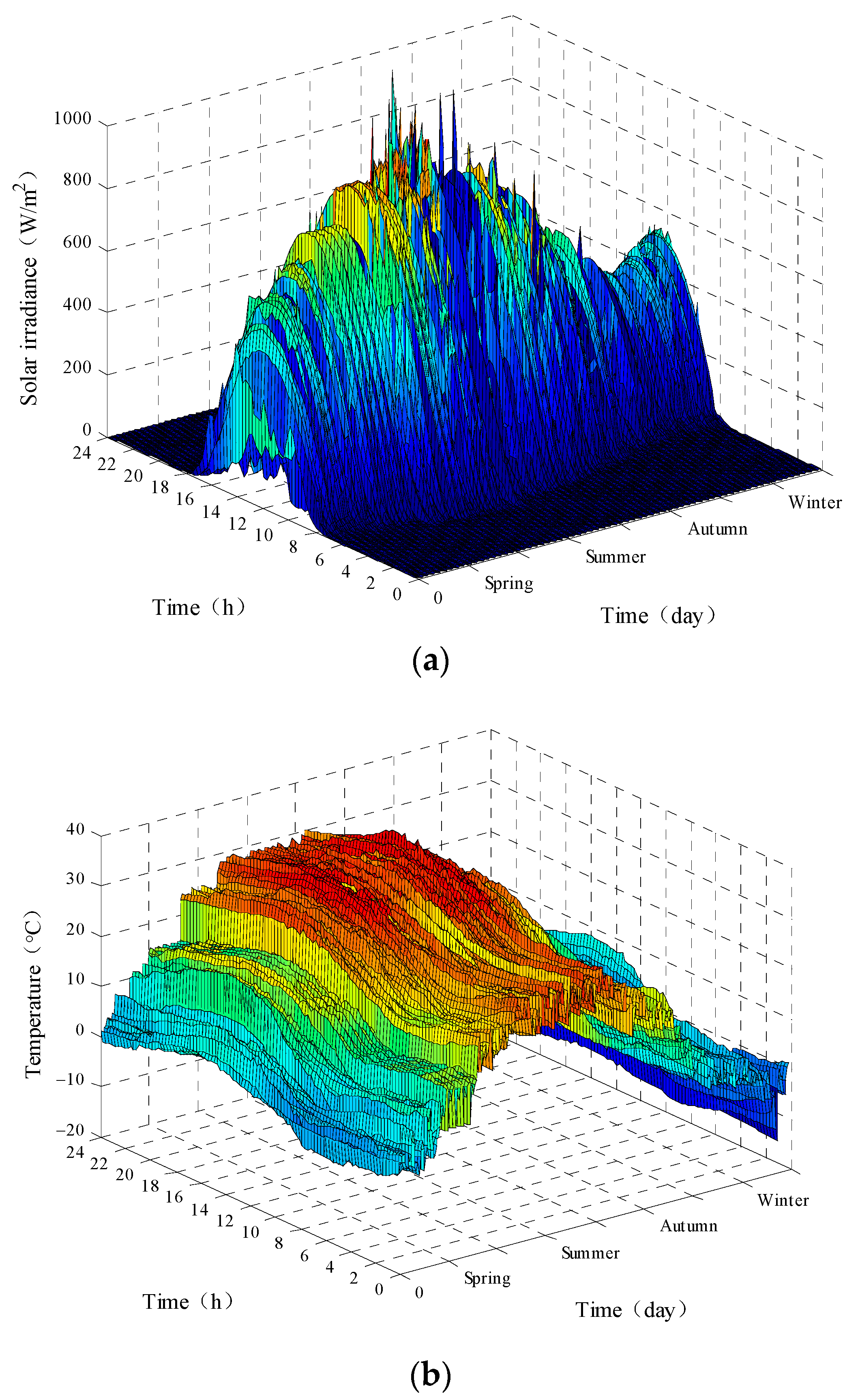
For the purpose of this study, an empirical PV plant located at the North China Electric Power University was analyzed. Its installed capacity is 9.5 kWp, with a data resolution of 15 min. Figure 2 shows the annual curves of solar irradiance and temperature of 2016, which demonstrates the strong effects from different seasons. The time series of solar irradiance and temperature has obvious characteristics in winter and summer, with a peak in summer and the valley in winter. The solar irradiance and temperature exhibit a nonlinear change with seasonal change.
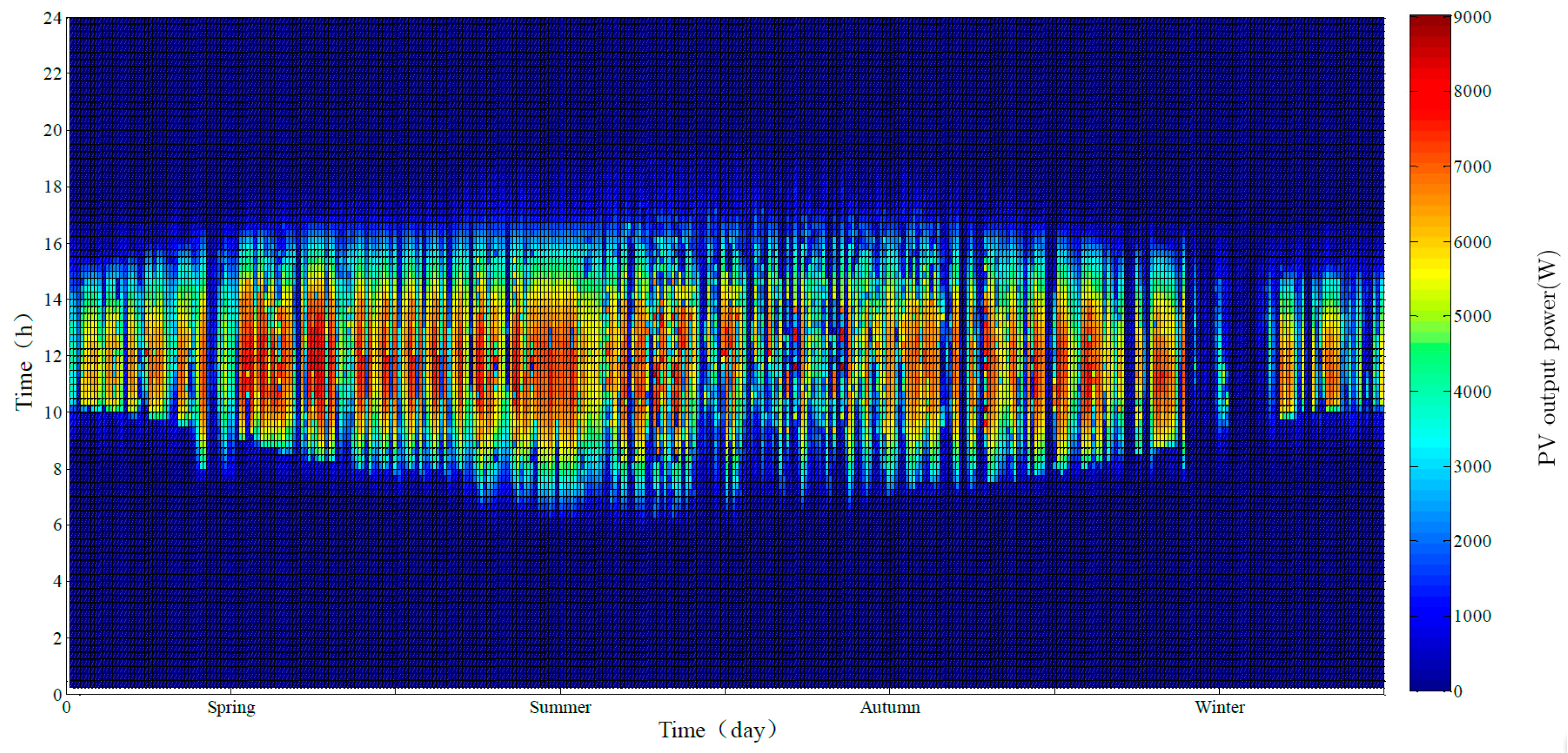
Figure 3 shows the time series diagram of annual output power of the PV plant in 2016. Under the combined effect of nonlinear solar irradiance and temperature, PV output power exhibited prominent nonlinear characteristics. Due to external factors such as climatic, meteorological and geographical conditions, PV output power shows periodic and nonlinear characteristics. The temporal time series of PV output power also changes in different seasons, becoming longer in summer and autumn when the sunshine duration is long, and relatively shorter in the spring and winter when the sunshine duration is short. The level of output power shows a high overall output value in summer, low output power in winter, and moderate output power in spring and autumn. The nonlinear characteristic of PV output power changes with time.

2.2. Influence of Internal Factors

Internal factors can affect the output of the PV plant in three aspects. First, for the overall PV plant, the installed tilt of PV modules and the arrangement and array spacing of PV modules can exert a fixed effect on the PV plant.
Second, internal factors can affect the performance degradation of PV modules. The actual performance of PV modules running outdoors continuously degrades. Normally, the annual average performance degradation rate of PV modules is about 0.8% [28]. According to the statistics on the data of 1920 sample points around the world in the past 30 years [28], the actual performance degradation of silicon module ranges from 0 to 4.2%. The performance degradation of PV modules caused by various factors may cause a PV plant to cease full operation. The performance degradation process of a PV plant is a nonlinear process. The main causes of performance degradation and failure of the PV modules after long-time field operation include [29]: breakage of PV cells, Ethylene-Vinyl Acetate (EVA) discoloration, wrinkling, delamination, and backing material cracks caused by local overheating, which are common during long-time PV plant operation. Due to changes in the performance degradation rate of modules and the failure of modules, the output characteristic of a PV plant is a nonlinear time-varying process.
Third, the efficiency η of PV modules is constantly changing under the influence of different temperatures and solar irradiance, as shown in Equation (1) [30].
η = η r e f [ 1 a 1 ( T t e m , c T t e m , r e f ) + a 2 ln ( G T / 1000 ) ]
where η r e f refers to the reference module efficiency, a 1 = 0.005 ; a 2 = 0.052 ; T t e m , r e f refers to the reference temperature (25 °C); G T refers to the surface solar radiance of silicon-based PV modules; and T t e m , c refers to the operating temperature of the PV modules.
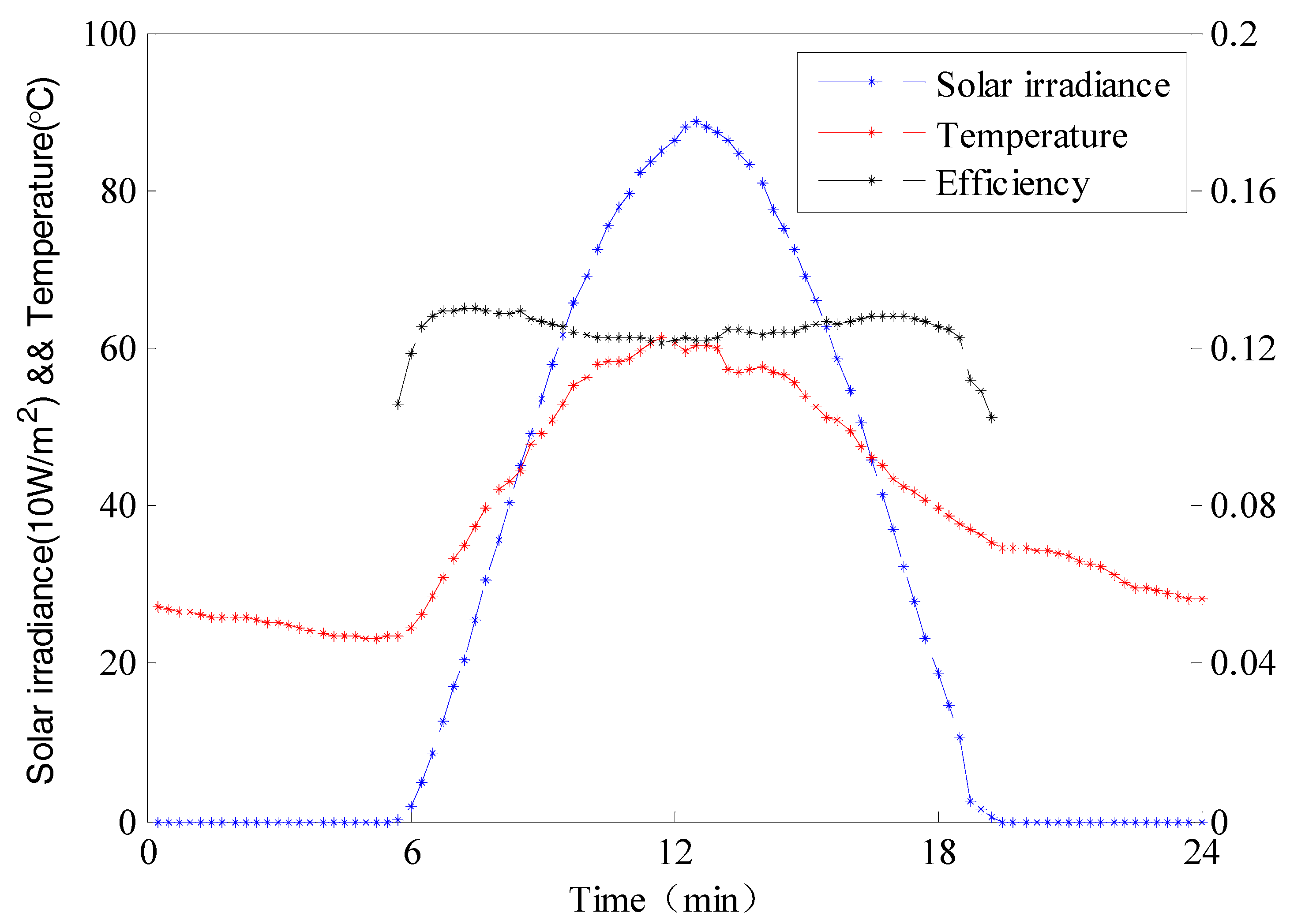
The correlation of the efficiency of PV modules and the temperature and radiance can be determined as described in Equation (1), and the result is shown in Figure 4. Obviously, the efficiency of PV modules has a complicated relationship with the actual irradiance and environment temperature.

2.3. Brief Summary

According to the analyses above, the fieldwork PV plant is subject to the influence of both external and internal factors. The characteristics of the PV plant itself constantly change under the excitation of continuously changing external factors, so the efficiency and output power of PV plant are characterized by obvious nonlinearity and time variance. These factors can cause a significant calculation error if PV power generation objects are not considered as dynamically changing in prediction modeling.

3. The Proposal of Improved Method

3.1. BP Neural Network Principle
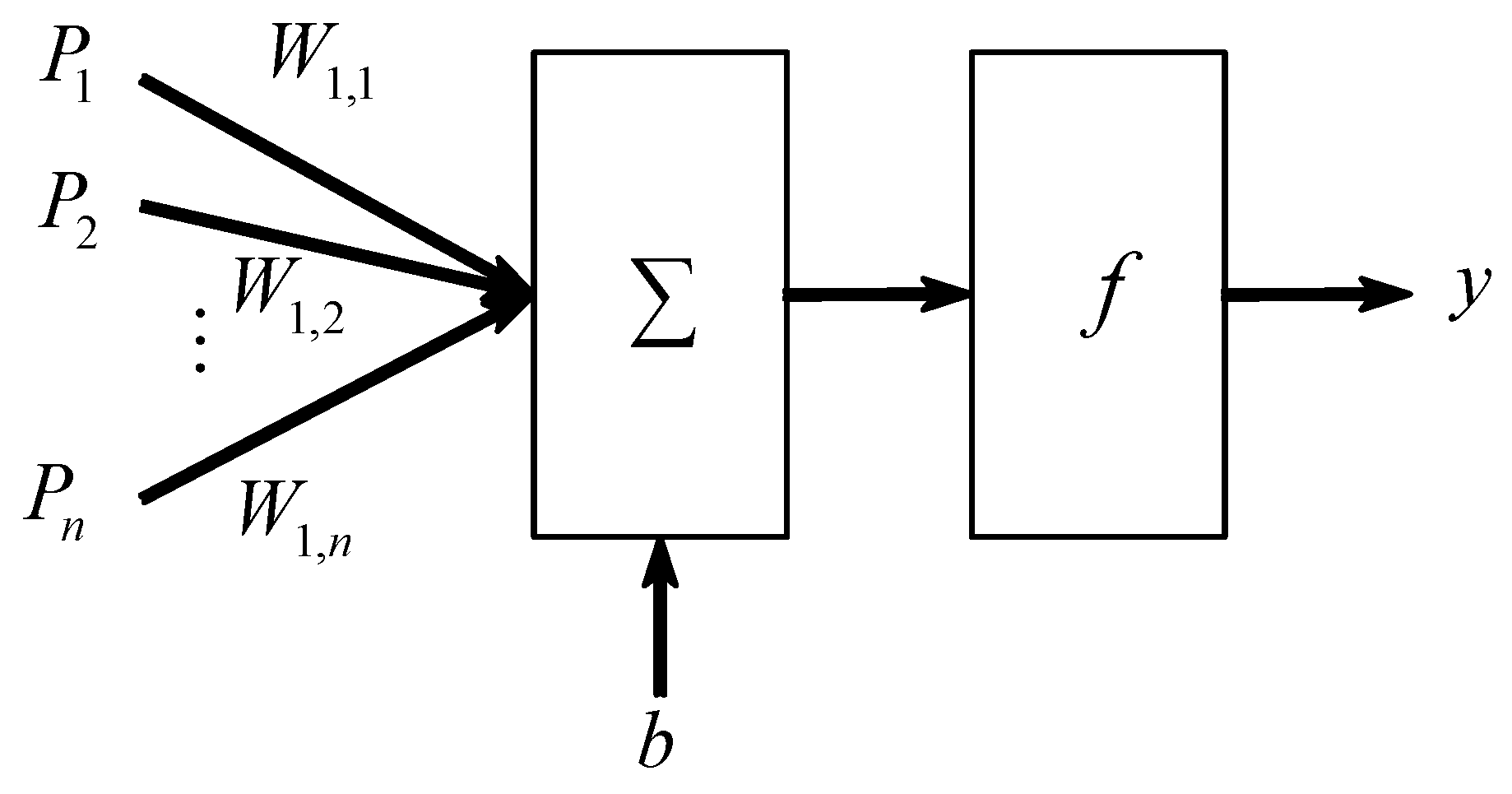
The BP neural network is one of the most widely applied algorithms [13]. It is a multilayer forward network for single-direction dissemination. Generally, a BP neural network consists of three layers or more, where the layers are fully connected with each other, but the neurons at each layer are independent. The model of the BP neural network is shown in Figure 5:
Figure 5. Model of back propagation (BP) neurons.
Energies 10 01542 g005
where V i refers to the ith input, of which the input vector is denoted by V; wi,j refers to the weight of the jth hidden layer node of the ith input, of which the input weight matrix is denoted by w; b refers to the threshold value of neuron; and f refers to transmission function. The output function is
y = f i n ( j = 1 R V i w i , j + b )
For a two-layer BP neural network, suppose k is the number of iterations, and the modifier equation of the weight and threshold value is
x ( k + 1 ) = x ( k ) α g ( k )
where x(k) refers to the link weight and threshold value between the two layers at the kth iteration, and α refers to learning rate.
g ( k ) = E ( k ) x ( k )
g ( k ) refers to the gradient of the output error E ( k ) of the kth iteration relative to the weight and the threshold value.
E ( k ) = 1 n S 2 j = 1 n i = 1 S 2 ( t i 2 y i 2 ( k ) ) 2
where n refers to the number of training samples; t refers to the target value; and y refers to the predicted value. The weight and threshold should be corrected successively until the total error meets the requirements.
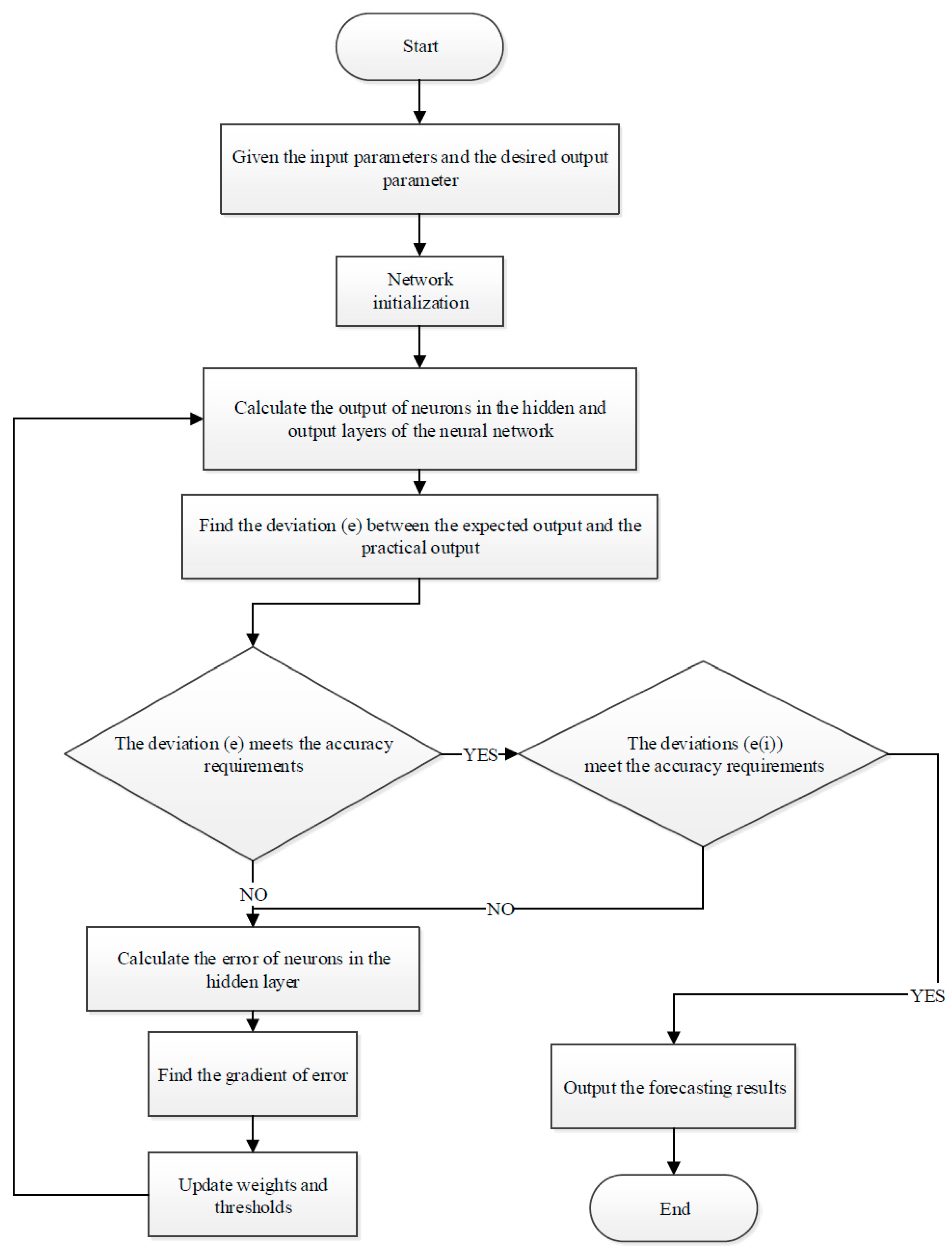
Figure 6 shows the flow of applying BP neural network in power forecasting. The input and output of a set of samples are converted into a nonlinear optimization problem, and the most common gradient descent method in optimization is adopted in a traditional BP neural network, which is effective to simulate and emulate nonlinear objects. However, this approach also has disadvantages:
  • The gradient descent and learning rate of a traditional neural network are slow, typically requiring thousands of training steps. Therefore, it may have a long-time error flat region.
  • Since the training process is long, it can only weakly dynamically track nonlinear time-varying objects.
  • Each training process is a brand new process for BP neural network, and its stability often suffers from the effect of initial weight value selection.
The algorithm flow chart of the BP neural network is:

3.2. Scrolling Time Window Technology

Assume that the input and output time-varying data sample set of the system is:
Z = { ( x 1 , y 1 ) , ( x 2 , y 2 ) , ( x 3 , y 3 ) , , ( x l , y l ) R d × R }
The samples of a region can be expressed as:
( x 1 , y 1 ) , ( x 2 , y 2 ) , ( x 3 , y 3 ) , , ( x k + 1 , y k + 1 ) , ( x k + 2 , y k + 2 ) , , ( x k + l , y k + l ) R d × R
Suppose there are L sets of continuously recording data, and the current state of the system is mainly described with L sets of recording data from a previous moment to the current moment. As the system runs, the state of the system continuously changes. To accurately reflect the current state of the system with the model, the newly-obtained input and output data should be utilized to update the parameters of the current system model. This is the basic principle of scrolling time window technology [31].
The old data that is less related to the current moment can be ignored, or the significance of the old data in the modeling process should be lowered. To do this, a modeling data interval of a fixed length of L with time scrolling is used. If a new piece of data is added, the oldest one will be removed from data array accordingly. As the system runs, the data interval is constantly updated, and the model is constantly updated by the new data. Since the scrolling data interval keeps changing, this is called a scrolling time window, as shown in Figure 7 below.
Suppose the moment of the current state is T + L, and the length of the modeling data is L, representing the time between moment T and the moment T + L. The model needs to be established based on the data in the L interval, and the next moment is predicted. At the next moment, moment T + L + 1, new measured data is added and the data at the moment T is discarded, so the model is based on the L interval from the moment T + 1 to the moment T + L + 1.
Therefore, the length of the interval is always L. In this way, the scrolling of the time window is realized.

3.3. The New Proposed Method

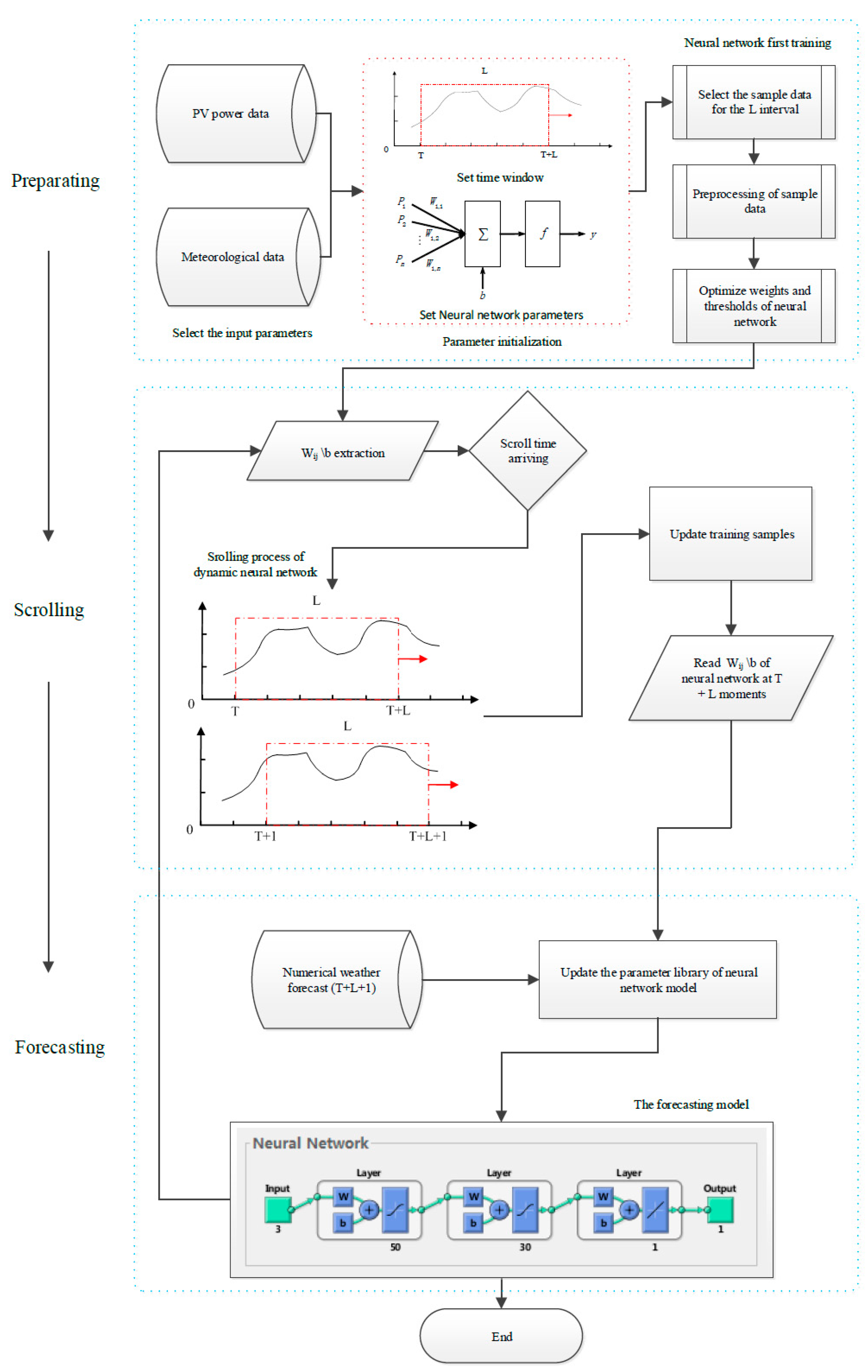
Modeling flow diagram of the dynamic neural network based on scrolling time window technology is shown in Figure 8, and the modeling steps are shown as following:
Step 1: Data preparation:
For a certain PV plant, its historical information can reflect the influence of various factors on the output power, such as the structure, arrangement, and performance degradation of PV plant. Scientific selection of input and output parameters and the sufficiency of training samples are of great significance to a BP neural network. For a BP neural network forecasting model, input variables include the environmental information of a PV plant, such as solar irradiance, temperature, and humidity, and the output layer is the output power sequence of the PV plant in the future.
Step 2: Initial training of neural network
The size L of the time window is also the size of BP neural-network training samples. This step builds a forecasting model with a five-layer BP neural network. The BP neural network consists of an input layer, an output layer, and three hidden layers, and the numbers of neurons at the three hidden layers are 50, 30, and 1, respectively. Sigmoid neuron activation function and gradient descent are adopted to train the network structure, and a genetic algorithm is adopted to optimize the initial weights and thresholds of the neural network.
There is an optimization process for the neural network to obtain the best initial weight value and thresholds.
Step 3: Scrolling updating of training samples:
The time window L should be determined based on the actual needs to contain sufficient samples to reflect the system characteristics and guarantee a faster learning rate. As the new forecasting time is reached, the time window moves forward, the data of the most recent training samples enters the time window, and the data at moment T is discarded.
Step 4: Scrolling training of neural network:
This step takes the weights and thresholds hold of the BP neural network at moment T + L as the initial parameters of the network at moment T + L + 1, and employ the latest training samples for neural network training.
The scrolling process keeps the weights and thresholds from previous training process and uses them as the initial values for the next training process; it ensures the fast convergence of the neural network algorithm and can effectively reduce the number of calculations. At the same time, it is most critical to avoid the random initialization of the neural network weights to ensure optimal calculation results.
Step 5: Scrolling forecasting process:
This step selects the environmental information of PV plant (T + L + 1) as inputs of the model, namely solar irradiance, temperature, and humidity from numerical weather prediction. Then, the PV output power at moment T + L + 1 can be forecasted based on the training result obtained via Step 4, and the BP neural network parameters are then stored as the initial parameters of the neural network for the next training process.

4. The Application and Result

4.1. Design of Experimental Method

A neural network learning algorithm depends upon the size of training sample data, and an excessively large or small training sample size affects the learning convergence and rate of convergence of the neural network. For this study, the length of the time window is determined by experiments. To this end, a period of 20 days [32] was compared to different time windows (L = 10, 15, 20, 25, 30, 35, 40 (days)). For comparison, the annual data of 2016 was divided into six groups and statistical analysis was performed.

4.2. Determination of Length of Time Window

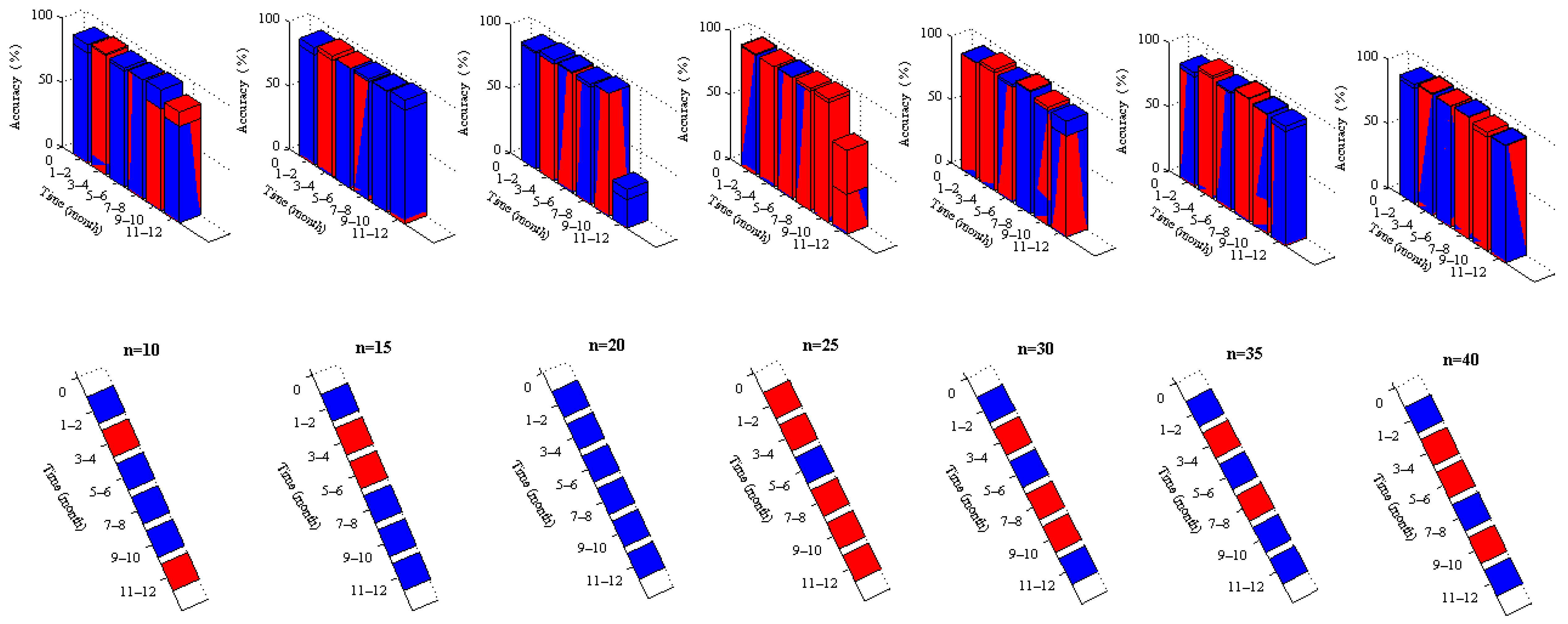
To determine a proper length of time window, the seven models were compared experimentally with the annual forecasting model from the perspective of prediction accuracy. Table 1 shows the training samples and test samples, and Table 2 shows the final calculation results. Figure 9 shows the bar diagrams of accuracies, and comparison of the side view and top view.
The following conclusions were made based on Table 2 and Figure 9.
The red bars in Figure 9 represent the prediction accuracy of prediction models with different scrolling time windows, and the blue ones represent the prediction accuracy of the annual forecasting model from the side view. The larger number of red blocks indicates higher model prediction accuracy corresponding to a certain time window from the top view. According to the given seven models in Figure 9, the prediction accuracy of the corresponding model was the highest for a 25-day time window. The 25-day model accuracy of five groups was higher than that of the annual forecasting model, and the accuracy of the other group was close to that of the annual forecasting model, with a difference of only 0.53% in the six experimental groups.
In the sixth experimental group, it was rainy, snowy, or cloudy from 21 November to 23 November, and cloudy and smoggy from 26 November to 28 November. During this period, the accuracy of the annual prediction model reduced to 30%. It is thus clear that the annual forecasting model works poorly under bad weather conditions (not sunny). However, the prediction effect is significantly improved once the 25-day scrolling forecasting model is adopted.

4.3. Performance Analysis of Algorithm

Table 3 presents the training time of models with different time windows, which indicates that:
  • As the length of time window extends, the quantity of sample data increases, and the training time of the model also increases gradually.
  • Compared with the training time (about 20 min) of the annual forecasting model, the training time of scrolling time window model is short, and the rate of convergence is fast.
  • Since the short-term forecasting of PV power requires that the time for single calculation is shorter than 5 min, the training time of a 25-day scrolling time window model is shorter than 2 min, which can meet the corresponding requirements, perform calculation quickly, and exhibit good performance.
To further verify the PV power forecasting method based on the neural network and scrolling time window, prediction of PV output power was made for five consecutive days with a 25-day forecasting model and an annual forecasting model. The predicted sample data obtained with an interval of 15 min from 1 October to 5 October was selected for analysis. To testing the effectiveness of the 25-day model, the forecasting results were evaluated with maximum error (MaxError), standard deviation (STD), root-mean-square error (RMSE), and mean absolute error (MAE) based on following equations
MaxError = M a x ( P M i P P i )
STD = i = 1 n ( P M i P m e a n ) 2 n
RMSE = i = 1 n | P M i P P i | C a p × n × 100 %
MAE = i = 1 n | P M i P P i | C a p × n × 100 %
Accuracy = 100 RMSE
where P M i is actual power at time i ; P P i is forecasted power; C a p is average operating capacity of the PV plant; and n is the number of sampled data. P m e a n refers to the arithmetic mean value of the forecasted power. Calculation of average operating capacity in PV plant is decided by the start power of the PV inverter, the rated installed capacity of PV system, and operation time. The definition is Equation (13).
C a p = c o u n t i f ( P M i P s ) n × P r
where P s is the start power of the PV inverter; P r is the rated installed capacity of PV system; and c o u n t i f represents the number of events that meet some condition.
The quantitative analysis results of the 25-day scrolling time window model and the annual forecasting model are shown in Table 4.
As presented in Table 4, the MaxError and STD describe the deviation degree of the predicted power and RMSE and MAE describe the whole error. Based on these measures of error, the 25-day model appears to be superior. Comparison of forecasting results is shown in Figure 10.

5. Conclusions

Due to the generation characteristics determined by the changing external environment and the performance degradation of PV modules with time, the PV power generation process has significant nonlinear and time-varying characteristics. In the paper, an adaptive BP neural network model adopting scrolling time window has been proposed to solve the problem. Via updating the modeling data of the BP neural network with the scrolling time window, the PV power forecasting model can be continuously updated, which is adaptive with time and the changing external environment. In the validation test, the forecasting performance in different time windows is evaluated. The results show that the 25-day forecasting model can improve the accuracy of ahead-day prediction and largely reduce the training time of a scrolling forecasting model, which is taken as the optimized time window to establish the PV power forecasting model. It suggests that the forecasting model of adaptive BP neural network with appropriate time windows can effectively represent the actual PV power generation characteristics and improve the PV power forecasting accuracy. Then, the proposed forecasting model is compared with the fixed model trained by the operation data over a whole year. The results show that the adaptive forecasting model has greater accuracy, superior to that of the fixed forecasting model. Overall, the proposed approach can improve the forecasting accuracy and also reduce the computation complexity of the BP neural network algorithm, which is very effective for the PV power forecasting application.

Acknowledgments

The authors would like to acknowledge the Fundamental Research Funds for the Central Universities “2016MS52, 2016MS31” and the Research Funds from State Grid Corporation of China “SGHE0000KXJS1700074”.

Author Contributions

All authors contributed to this work by collaboration. Honglu Zhu is the first author in this manuscript. All authors revised and approved for the publication.

Conflicts of Interest

The authors declare no conflict of interest.

Nomenclature

Capaverage operating capacity
Ethe output error
Gsolar irradiance (W/m2)
GTsolar irradiance on module plane (W/m2)
Kthe number of iterations
Lthe length of the modeling data
MAEmean absolute error
MaxErrormaximum error
Pelectrical power (W)
RMSEroot mean square error
STDstandard deviation
Ttemtemperature (°C)
Ttem,ccell/module operating temperature (°C)
Vthe input variable
Wthe weight
Zthe input and output time-varying data sample set
Subscripts-
ccell (module)
Mithe measured value at time i.
meanthe average value
nsample size
Pithe predicted value at time i.
rthe rated state
refreference value, at reference conditions
sthe start state
Ton module’s tilted plane

References

  1. Raza, M.Q.; Nadarajah, M.; Ekanayake, C. On recent advances in PV output power forecast. Sol. Energy 2016, 136, 125–144. [Google Scholar] [CrossRef]
  2. Mellit, A.; Pavan, A.M.; Lughi, V. Short-term forecasting of power production in a large-scale photovoltaic plant. Sol. Energy 2014, 105, 401–413. [Google Scholar] [CrossRef]
  3. Eltigani, D.; Masri, S. Challenges of integrating renewable energy sources to smart grids: A review. Renew. Sustain. Energy Rev. 2015, 52, 770–780. [Google Scholar] [CrossRef]
  4. Soman, S.S.; Zareipour, H.; Malik, O.; Mandal, P. A review of wind power and wind speed forecasting methods with different time horizons. In Proceedings of the North Am. Power Symp. (NAPS), Arlington, TX, USA, 26–28 September 2010; pp. 1–8. [Google Scholar]
  5. Graditi, G.; Ferlito, S.; Adinolfi, G. Comparison of photovoltaic plant power production prediction methods using a large measured dataset. Renew. Energy 2016, 90, 513–519. [Google Scholar] [CrossRef]
  6. Piliougine, M.; Elizondo, D.; Mora-Lo’pez, L.; Sidrach-de-Cardona, M. Modelling photovoltaic modules with neural networks using angle of incidence and clearness index. Prog. Photovolt. Res. 2015, 23, 513–523. [Google Scholar] [CrossRef]
  7. Huang, L.; Shu, J.; Jiang, G.; Zhang, J. Photovoltaic generation forecast based on multidimensional time-series and local support vector regression in microgrids. Autom. Electr. Power Syst. 2014, 38, 19–24. [Google Scholar]
  8. Ding, M.; Xu, N. A Method to Forecast Short-Term Output Power of Photovoltaic Generation System Based on Markov Chain. Power Syst. Technol. 2011, 35, 152–157. [Google Scholar]
  9. Almonacid, F.; Pérez-Higueras, P.J.; Fernández, E.F.; Hontoria, L. A methodology based on dynamic artificial neural network for short-term forecasting of the power output of a PV generator. Energy Convers. Manag. 2014, 85, 389–398. [Google Scholar] [CrossRef]
  10. Antonanzas, J.; Osoriob, N.; Escobar, R.; Urraca, R.; Martinez-de-Pison, F.J.; Antonanzas-Torres, F. Review of photovoltaic power forecasting. Sol. Energy 2016, 136, 78–111. [Google Scholar] [CrossRef]
  11. Zhu, H.; Li, X.; Sun, Q.; Nie, L.; Yao, J.; Zhao, G. A power prediction method for photovoltaic power plant based on wavelet decomposition and artificial neural networks. Energies 2015, 9, 11. [Google Scholar] [CrossRef]
  12. Ye, L.; Chen, Z.; Zhao, Y. Photovoltaic power forecasting model based on genetic algorithm and fuzzy radial basis function neural network. Autom. Electr. Power Syst. 2015, 39, 16–22. [Google Scholar]
  13. Wang, X.; Zhou, X.; Xing, J.; Yang, J. A prediction method of PV output power based on the combination of improved grey back propagation neural network. Power Syst. Prot. Control 2016, 44, 81–87. [Google Scholar]
  14. Zhang, G. Time series forecasting using a hybrid ARIMA and neural network model. Neurocomputing 2003, 50, 159–175. [Google Scholar] [CrossRef]
  15. Vaz, A.G.R.; Elsinga, B.; van Sark, W.; Brito, M.C. An artificial neural network to assess the impact of neighbouring photovoltaic systems in power forecasting in Utrecht, The Netherlands. Renew. Energy 2016, 85, 631–641. [Google Scholar] [CrossRef]
  16. Ferlito, S.; Adinolfi, G.; Graditi, G. Comparative analysis of data-driven methods online and offline trained to the forecasting of grid-connected photovoltaic plant production. Appl. Energy 2017, 205, 116–129. [Google Scholar] [CrossRef]
  17. Li, C.; Liu, X.; Cao, Y.; Zhang, P.; Shi, H.; Ren, L.; Kuang, Y. A time-scale adaptive dispatch method for renewable energy power supply systems on islands. IEEE Trans. Smart Grid 2016, 7, 1069–1078. [Google Scholar] [CrossRef]
  18. Eleonora, R.S.; Roberto, G.; Gaetano, Z.; Gallea, R.; Quang, N.N. A self-adapting approach for forecast-less scheduling of electrical energy storage systems in a liberalized energy market. Energies 2013, 6, 5738–5759. [Google Scholar]
  19. Dash, P.K.; Liew, A.C.; Ramakrishna, G. Power-demand forecasting using a neural network with an adaptive learning algorithm. IEE Proc. Gener. Transm. Distrib. 1995, 142, 560–568. [Google Scholar] [CrossRef]
  20. Liu, K.; Subbarayan, S.; Shoults, R.R.; Manry, M.T.; Kwan, C.; Lewis, F.I.; Naccarino, J. Comparison of very short-term load forecasting techniques. IEE Trans. Power Syst. 1996, 11, 877–882. [Google Scholar] [CrossRef]
  21. Xu, Y.; Milanović, J.V. Day-Ahead prediction and shaping of dynamic response of demand at bulk supply points. IEEE Trans. Power Syst. 2016, 31, 3100–3108. [Google Scholar] [CrossRef]
  22. Rosato, A.; Rosa, A.; Rodolfo, A.; Araneo, R.; Panella, M. Prediction in photovoltaic power by neural networks. Energies 2017, 10, 1003. [Google Scholar] [CrossRef]
  23. Dolara, A.; Grimaccia, F.; Leva, S.; Mussetta, M.; Ogliari, E. A physical hybrid artificial neural network for short term forecasting of PV plant power output. Energies 2015, 8, 1138–1153. [Google Scholar] [CrossRef] [Green Version]
  24. Al-Messabi, N.; Goh, C.; El-Amin, I.; Li, Y. Heuristically enhanced dynamic neural networks for structurally improving photovoltaic power forecasting. In Proceedings of the 2014 International Joint Conference on Neural Networks (IJCNN), Beijing, China, 6–11 July 2014. [Google Scholar]
  25. Ceci, M.; Corizzo, R.; Fumarola, F.; Malerba, D.; Rashkovska, A. Predictive modeling of PV energy production: How to set up the learning task for a better prediction. IEEE Trans. Ind. Inform. 2017, 13, 956–966. [Google Scholar] [CrossRef]
  26. Saberian, A.; Hizam, H.; Radzi, M.A.M.; Kadir, M.Z.A.A.; Mirzaei, M. Modelling and prediction of photovoltaic power output using artificial neural networks. Int. J. Photoenergy 2014, 2014. [Google Scholar] [CrossRef]
  27. Izgi, E.; Öztopal, A.; Yerli, B.; Kaymak, M.K.; Şahin, A.D. Short-mid-term solar power prediction by using artificial neural networks. Sol. Energy 2012, 86, 725–733. [Google Scholar] [CrossRef]
  28. Jordan, D.C.; Kurtz, S.R. Photovoltaic degradation rates—An analytical review. Prog. Photovolt. Res. Appl. 2013, 21, 12–29. [Google Scholar] [CrossRef]
  29. Zheng, H.; Hu, B.; Shen, H.; Ge, W. Analysis of performance and degradation of silicon PV modules after long term operation. Acta Energ. Sol. Sin. 2012, 33, 614–617. [Google Scholar]
  30. Skoplaki, E.; Palyvos, J.A. On the temperature dependence of photovoltaic module electrical performance: A review of efficiency/power correlations. Sol. Energy 2009, 83, 614–624. [Google Scholar] [CrossRef]
  31. Wang, Y.; Wang, J.; Li, B.; Fan, H. The window-sliding forecast on the time series of the parameter-varying chao tic system using neural networks. J. Wuhan Univ. Technol. 2010, 34, 456–459. [Google Scholar]
  32. Phua, S.K. Data Base Preparation in Power Systems Management: Measurement Selection, Short-Term Load Prediction and Load Modeling; Monash University: Melbourne, Victoria, Australia, 1977. [Google Scholar]
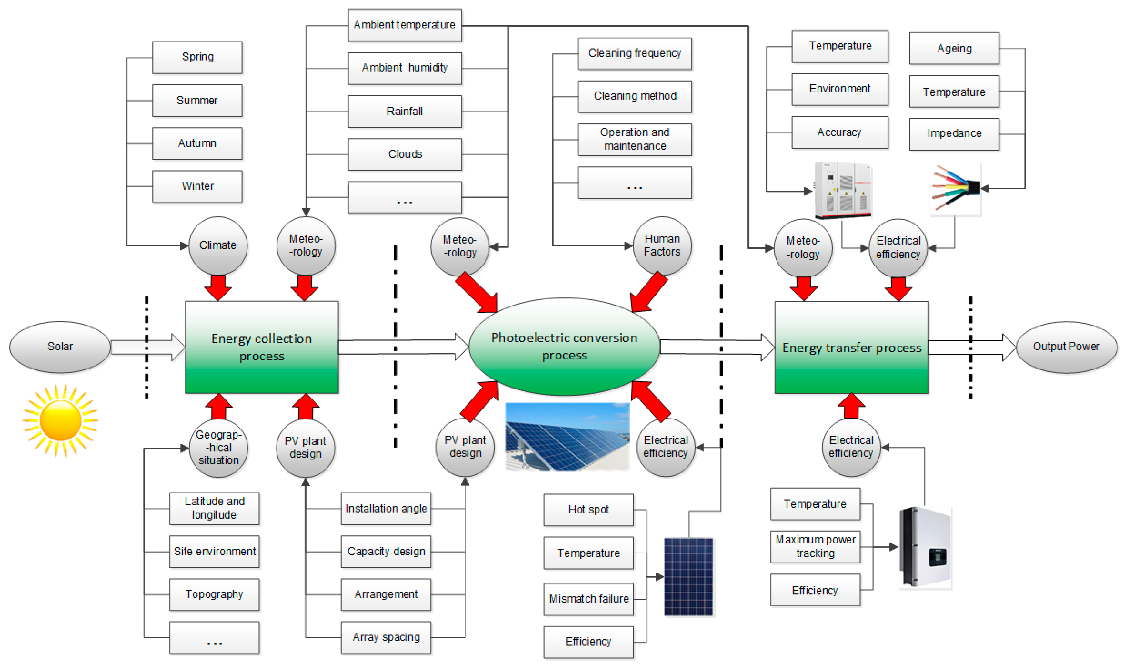
Figure 1. Determinants of photovoltaic (PV) plant output power.
Energies 10 01542 g001
Figure 2. Nonlinear characteristic of external input. (a) Annual solar irradiance time series of 2016; (b) Annual temperature time series of 2016.
Energies 10 01542 g002
Figure 3. Time series characteristics of annual output power of 2016.
Energies 10 01542 g003
Figure 4. Efficiency characteristics of silicon-based PV modules at different temperatures and irradiance conditions.
Energies 10 01542 g004
Figure 6. Power forecasting flow chart with a BP neural network.
Energies 10 01542 g006
Figure 7. Schematic diagram of a scrolling time window.
Energies 10 01542 g007
Figure 8. Modeling flow diagram of the dynamic neural network based on scrolling time window technology.
Energies 10 01542 g008
Figure 9. Comparison of prediction accuracy between models with different time windows and the annual model.
Energies 10 01542 g009
Figure 10. Comparison of forecasting results.
Energies 10 01542 g010
Table 1. Selection of experimental data.
Sample DataL = 10L = 15L = 20L = 25L = 30L = 35L = 40
Group 1Training1–10 January1–15 January1–20 January1–25 January1–30 January1–4 January1 January–14 February
Test11–13 January16–18 January21–23 January26–28 January31 January–2 February5–7 February15–17 February
Group 2Training1–10 March1–15 March1–20 March1–25 March1–30 March1 March–4 April1 March–14 April
Testing11–13 March16–18 March21–23 March26–28 March31 March–2 April5–7 April15–17 April
Group 3Training1–10 May1–15 May1–20 May1–25 May1–30 May1 May–4 June1 May–14 June
Testing11–13 May16–18 May21–23 May26–28 May31 May–2 June5–7 June15–17 June
Group 4Training1–10 July1–15 July1–20 July1–25 July1–30 July1 July–4 August1 July–14 August
Testing11–13 July16–18 July21–23 July26–28 July31 July–2 August5–7 August15–17 August
Group 5Training1–10 September1–15 September1–20 September1–25 September1–30 September1 September–5 October1 September–15 October
Testing11–13 September16–18 September21–23 September26–28 September1–3 October6–8 October16–18 October
Group 6Training1–10 November1–15 November1–20 November1–25 November1–30 November1 November–5 December1 November–15 December
Testing11–13 November16–18 November21–23 November26–28 November1–3 December6–8 December16–18 December
Footnote: The data of 366 days in 2016 was taken as the annual model training data, and the test data is the corresponding data of each model in different periods.
Table 2. Selection of experimental data.
GroupingAccuracy (%)
L = 10L = 15L = 20L = 25L = 30L = 35L = 40
Group 185.1986.690.2194.1691.4685.489.74
One year91.7492.2891.4593.2191.8888.6592.7
Group 293.8494.9190.7993.7995.5395.4595.09
One year92.6591.4194.193.7392.9193.4394.21
Group 389.8394.5193.1194.4191.0591.0694.55
One year92.1494.3594.0794.9493.0392.4694.21
Group 492.0993.3191.2295.3597.5396.6995.18
One year92.3595.393.9693.0496.4896.1395.52
Group 579.0194.995.7696.2493.6893.3292.44
One year93.6295.4295.8593.4890.9193.9688.7
Group 685.8789.3322.1965.479.9689.1791.27
One year74.6697.230.1731.0591.7193.1291.87
Table 3. Training time of models with different time windows.
GroupingTraining Time (s)
L = 10L = 15L = 20L = 25L = 30L = 35L = 40
Group 158.7671.5679.2290.78113.10126.15150.69
Group 254.3472.8282.72101.05126.23135.25158.69
Group 361.7864.0389.3094.44118.27139.39151.50
Group 458.7567.4977.1791.80110.00123.69138.30
Group 560.9574.7891.40109.30172.88154.26162.03
Group 656.2771.0478.9591.79287.36137.73139.91
Average58.4870.2983.1396.53154.64136.08150.19
One yearAverage = 1175.00
Table 4. Error analysis. MaxError: maximum error; STD: standard deviation; RMSE: root-mean-square error; MAE: mean absolute error.
Training DataTesting DataMaxError (W)STDError (W)RMSE (%)MAE (%)
1–25 January26–28 January1749.05349.565.842.86
One year26–28 January2016.98399.266.793.50
1–25 March26–28 March2278.84420.116.213.30
One year26–28 March2123.48410.976.273.58
1–25 May26–28 May1367.68261.365.593.48
One year26–28 May908.60233.445.063.22
1–25 July26–28 July947.60181.094.652.71
One year26–28 July1217.28275.836.963.91
1–25 September26–28 September1114.98221.623.762.00
One year26–28 September1679.96383.256.523.50
1–25 November26–28 November3398.66555.2234.6015.26
One year26–28 November4557.201101.7768.9530.94