Probabilistic Load-Flow Analysis of Biomass-Fuelled Gas Engines with Electrical Vehicles in Distribution Systems

Abstract

Feeding biomass-fueled gas engines (BFGEs) with olive tree pruning residues offers new opportunities to decrease fossil fuel use in road vehicles and electricity generation. BFGEs, coupled to radial distribution systems (RDSs), provide renewable energy and power that can feed electric vehicle (EV) charging stations. However, the combined impact of BFGEs and EVs on RDSs must be assessed to assure the technical constraint fulfilment. Because of the stochastic nature of source/load, it was decided that a probabilistic approach was the most viable option for this assessment. Consequently, this research developed an analytical technique to evaluate the technical constraint fulfilment in RDSs with this combined interaction. The proposed analytical technique (PAT) involved the calculation of cumulants and the linearization of load-flow equations, along with the application of the cumulant method, and Cornish-Fisher expansion. The uncertainties related to biomass stock and its heating value (HV) were important factors that were assessed for the first time. Application of the PAT in a Spanish RDS with BFGEs and EVs confirmed the feasibility of the proposal and its additional benefits. Specifically, BFGEs were found to clearly contribute to the voltage constraint fulfilment. The computational cost of the PAT was lower than that associated with Monte-Carlo simulations (MCSs).

1. Introduction

In the world today, there is great concern about the possible effects of climate change. For this reason, international policy [1,2,3] predicts a reduction in the use of fossil fuels, and the electricity sector is gradually switching to renewable power sources. Moreover, the internal combustion engines in vehicles are slowly being replaced by electric motors [4]. Nevertheless, it is also true that fossil fuels are still widely used to power road vehicles and to generate electricity.

In this context, biomass has become an attractive option for public and policymakers [5]. Some authors even affirm that biomass is the best source of renewable power [6]. Residual biomass obtained from tree pruning is one of the renewable and sustainable sources that can be used for producing electricity. Certain studies [7,8] underline its low use/potential ratio, and highlight the need to make its use more widespread.

Over eight million hectares of olive trees are cultivated worldwide, especially in the Mediterranean countries, where more than 97% of the world’s olive oil is produced. The three major olive oil producers are Spain, Italy, and Greece [9,10]. Olive tree pruning residues are an autochthonous renewable energy source that farmers generally dispose of by burning. However, this practice is gradually changing since olive growers must now comply with stricter regulations regarding the sustainable management of residual biomass [11]. New technologies that can be used to produce electricity from this biomass [6,9] include the following: direct combustion, co-firing, gasification, pyrolysis, anaerobic digestion, and fermentation. However, the most widespread technology is direct combustion with BFGEs [12,13], in which BFGEs are coupled to the grid by small synchronous generators [12]. On the other hand, the large-scale use of EVs involves the massive integration of EV charging stations in traditional RDSs. This is a source of numerous technical challenges [14].

Although the use of olive tree pruning residues in BFGEs as a renewable power source in future RDSs with EVs will make the generating system more sustainable, the assessment of this proposal, by analyzing the technical impact of the BFGE and EV interaction on RDSs, is problematic because of the stochastic nature of the source/load involved. Evidently, the biomass supply chain, from tree pruning to energy generation, is affected by uncertainties such as unpredictable biomass quality [15] and quantity [16]. The EV charging load on RDSs also presents uncertainties [17]. Consequently, it is necessary to implement a probabilistic approach, which is capable of accurately characterizing RDS performance taking into account the possible uncertainties in the inputs variables. Probabilistic approaches are widely applied in the analysis of electric power systems [18].

There are few studies that focus on the uncertainties of the biomass supply chain [19,20,21,22,23]. Some papers (e.g., [24]) have assessed the adverse technical impacts of BFGEs, working as electrical generators, on RDSs. Nonetheless, a deterministic approach was used for these assessments. No reference specifically incorporated models and methods that were able to quantify the uncertainty of biomass stock and its HV. Accordingly, the impact of the input uncertainties on the results may not have accurately estimated. In contrast, many probabilistic studies analyzed the potentially negative technical impacts that EVs originate in RDSs: (i) thermal loading [25,26,27,28,29,30,31] (ii) node voltage profile [14,25,28,32,33,34,35,36,37]; (iii) power line losses [17,25,30,35,38].

Until now, the negative technical impacts of EVs have been minimized by demanding interconnection requirements [14]. Such requirements were based on deterministic assessments for worst-case scenarios. Nonetheless, these assessments are unable to objectively specify when a technical constraint is fulfilled, in other words, when the time-variant values of an RDS output variable (e.g., node voltage) can exceed the standard limit in the regulation. An accurate assessment of the technical impact of BFGE and EV interaction on RDSs should include the investigation of all possible inputs. As a main technical constraint, distribution network operators (DNOs) in European countries use the ±10%-threshold [39] as a limit for the voltage magnitude. Nonetheless, Spanish Royal Decree 1955/2000 [40] sets a restrictive threshold of ±7%. Both assessments are based on measurements averaged at 10-min intervals.

A review of the literature [19,20,21,22,23,24,25,26,27,28,29,30,31,32,33,34,35,36,37,38] indicates that the BFGE and EV impact on RDSs has still not been assessed from a probabilistic perspective. The first major shortcoming is evidently the fact that probabilistic approaches have never been applied to BFGEs. The second is that probability of occurrence has not been considered in the evaluation of the technical impact of EVs on RDSs. Therefore, the probability distribution of the RDS output variables was not calculated.

This study further develops the research reported in [41] and presents an innovative analytical technique that is able to accurately assess the combined impact of BFGEs and EVs on RDSs by focusing on voltage constraint fulfilment. The proposed analytical technique (PAT) was found to overcome the previously mentioned shortcomings. Thus, for different scenarios the true probabilities of voltage violation in the regulations were determined from the probability distributions of the RDS output variables. This simultaneously takes into account the BFGE probabilistic model and the probabilistic model advanced in this study for EVs.

The rest of the paper is organized as follows: Section 2 gives an overview of the statistical background upon which this research is based. After a concise description of the probabilistic models in Section 3, Section 4 outlines the PAT used in this study. Section 5 describes the test system, followed by a presentation of the simulation results in Section 6. Finally, Section 7 gives the conclusions that can be derived from this study.

2. Moments and Cumulants of a Random Variable

For a better understanding of the PAT, this section provides a short introduction to probability theory, which also justifies the use of moments and cumulants.

The moments of a random variable are the expected values of certain functions of this variable, which characterize its probability distribution. For a multivariable random variable $\mathit{X}(={[{\mathit{X}}_{\mathbf{1}},{\mathit{X}}_{\mathbf{2}},\dots ,{\mathit{X}}_{{\mathit{n}}_{\mathit{r}\mathit{v}}}]}^T)$ with probability density function (PDF) $f_{\mathit{X}}\left(\mathit{X}\right)$ (continuous variable), or probability mass function (PMF), $f_{\mathit{X}}^{*}\left(\mathit{X}\right)$ (discrete variable), its moment of order one, two and r is defined as [42,43]:

$$\begin{array}{l}{\alpha }_{\mathit{X}}^{\stackrel{1}{\overleftrightarrow{i_i}}}=E\left[X_{i_i}\right];{\alpha }_{\mathit{X}}^{\stackrel{2}{\overleftrightarrow{i_i{i}_j}}}=E\left[X_{i_i}{X}_{i_j}\right];{\alpha }_{\mathit{C}}^{\stackrel{r}{\overleftrightarrow{i_i\dots i_r}}}=E\left[X_{i_i}\stackrel{r}{\overleftrightarrow{\dots }}{X}_{i_r}\right]\\ -\mathrm{continuous}\mathrm{case}--\mathrm{discrete}\mathrm{case}-\\ {\alpha }_{\mathit{X}}^{\stackrel{r}{\overleftrightarrow{i_i\dots i_r}}}={\displaystyle \underset{-\infty }{\overset{\infty }{\int }}\stackrel{r}{\overleftrightarrow{\dots }}}{\displaystyle \underset{-\infty }{\overset{\infty }{\int }}{X}_{i_i}\dots X_{i_r}\cdot f_{\mathit{X}}\left(\mathit{X}\right)d\mathit{X}};{\alpha }_X^{\stackrel{r}{\overleftrightarrow{i_i\dots i_r}}}={\displaystyle \sum _{i_i=1}^{\infty }\stackrel{r}{\overleftrightarrow{\dots }}}{\displaystyle \sum _{i_r=1}^{\infty }{X}_{i_1}\dots X_{i_r}\cdot f_{\mathit{X}}^{*}\left(\mathit{X}\right)}\end{array}$$

(1)

The cumulants of a distribution are a set of constants that provide an alternative to the moments to its characterization [43]. Unlike the moments, these cumulants are not directly ascertainable by summatory or integrative processes − as in Equation (1). To find them, it is thus necessary to determine the moments and then employ relationship formulas [43].

The PAT (see Section 4) is used to concisely model and characterize input random variables as well to perform a load-flow in an RDS to determine its output random variables. This is accomplished by applying linearized load-flow equations, and finally reconstructing distributions through the use of approximations. For calculation purposes, the PAT must know the moments and cumulants of the input and output random variables. Nonetheless, the PAT works better with cumulants than moments for the following reasons [42]: (i) the Cornish-Fisher expansion used for approximations to the distributions is best expressed with cumulants; (ii) most statistical calculations with cumulants are simpler than calculations with moments. This is the case when determining the cumulants of output variables from the cumulants of input variables subject to linear transformation. Thus, let Z be a random variable that is a linear combination of a multivariate random variable, X, given by:

$$\mathit{Z}={\displaystyle \sum _{i_i=1}^{n_{rv}}{a}_{i_i}}\cdot {\mathit{X}}_{i_i}$$

(2)

In the application of the cumulant method [42], the r-order cumulant of the random variable Z can be expressed as a function of the cumulants of the variable X as:

$${\kappa }_{\mathit{Z}}^{\stackrel{r}{\overleftrightarrow{1\dots 1}}}={\displaystyle \sum _{i_i=1}^{n_{rv}}\stackrel{r}{\overleftrightarrow{\dots }}{\displaystyle \sum _{i_r=1}^{n_{rv}}{a}_{i_i}\stackrel{r}{\overleftrightarrow{\dots }}{a}_{i_r}\cdot }}{\kappa }_{\mathit{X}}^{\stackrel{r}{\overleftrightarrow{i_i\dots i_r}}}$$

(3)

3. Probabilistic Models

3.1. Power Model of a BFGE

The use of olive tree pruning residues as fuel in BFGEs for electrical applications requires the accurate quantification of both the amount of the biomass available in a specific area as well as its HV. The annual biomass quantity depends on local factors such as the architecture of the tree type in question, variety, aim of the pruning, age of the plants, tree growing space, fruit yield, pruning intensity (annual, biennial), and irrigation [11,16]. On the other hand, the quality of this biomass is determined by its physical and chemical characteristics. This quality is usually characterized by HV that is affected by local factors, such as the characteristics of the cultivation area (geographical and ecological characteristics), growth conditions, climate, harvesting methods, transportation methods, handling and warehousing operations [15], as well as the biomass moisture content. The HV reflects the energy content of the biomass in a standardized fashion [6]. It is often expressed as the higher HV or lower HV, also known as the net HV [6]. Although the HV can be determined directly, an easier and less expensive alternative is to use any of various models [6] whose predictions are based on variables.

The biomass supply chain from olive tree pruning to energy generation by BFGE is thus affected by local environmental uncertainties, outside of the energy production process. These uncertainties are directly related to the unpredictable quantity and quality of the biomass. These sources of uncertainty can be characterized by two random variables: (i) the annual net density of the dry biomass D; (ii) the higher HV of the biomass ${\mathit{H}}_{\mathit{b}}$.

The annual net density of biomass D can be assumed to be a random variable with a normal distribution [44,45,46]. This density ranges from 9.26 to 25 kg dry biomass tree⁻¹ [7,16,44,45,46,47,48,49]. For example, according to one very detailed study [16], olive tree varieties can be classified in two groups for annual pruning: high residual biomass productivity (average yield 10.5 kg tree⁻¹) and low productivity (average yield 3.5 kg tree⁻¹). There were no differences in biennial pruning. This means that in Mediterranean areas, the residual biomass from olive tree pruning reached an average 1.31 t ha⁻¹ in annual pruning.

The higher HV of the biomass H_b is assumed to be a random variable with a normal distribution [50,51,52]. Generally, the average higher HV on a dry basis is approximately 3.90–5.01 MJ t⁻¹ [47,50,51,52]. These higher HVs were found to be similar to those of agricultural residues (4.16–4.72 MJ t⁻¹ [50]) and to woody material (5.00–5.27 MJ t⁻¹ [50]).

In this study, the electric power of a BFGE was determined by means of a stochastic model which takes into account electrical and thermal requirements and depends on technological factors (set of biomass conversion processes). Furthermore, the model considers the local random variables which determine the annual amount of biomass available and its higher HV. Thus, the random power of a BFGE at any xth 10-min interval of the day (t_x) and nth RDS node $(n=1,\dots ,n_{bfge})$ is given by:

$${\mathit{p}}_{\mathit{b}\mathit{f}\mathit{g}\mathit{e},\mathit{n},\mathbf{10}-\mathit{m}\mathit{i}{\mathit{n}}_{{\mathit{t}}_{\mathit{x}}}}=\frac{\eta \cdot A_n\cdot {\tau }_n\cdot {\mathit{D}}_n\cdot {\mathit{H}}_{{\mathit{b}}_n}}{T_r}$$

(4)

The random variables ${\mathit{D}}_n$ and ${\mathit{H}}_{{\mathit{b}}_n}$ can be considered independent. Consequently, the probabilistic distribution of BFGE power, constructed as the distribution of the product of two random variables with known Gaussian distributions, can be obtained by the moments of ${\mathit{D}}_n$ and ${\mathit{H}}_{b_n}$ as follows [53]:

$$E\left[p_{bfge,n}\stackrel{r}{\overleftrightarrow{\dots }}{p}_{bfge,n}\right]=E\left[D_n\stackrel{r}{\overleftrightarrow{\dots }}{D}_n\right]\cdot E\left[H_{b_n}\stackrel{r}{\overleftrightarrow{\dots }}{H}_{b_n}\right];{\alpha }_{p_{\mathit{b}\mathit{f}\mathit{g}\mathit{e},\mathit{n}}}^{\stackrel{r}{\overleftrightarrow{1\dots 1}}}={\alpha }_{{\mathit{D}}_n}^{\stackrel{r}{\overleftrightarrow{1\dots 1}}}\cdot {\alpha }_{{\mathit{H}}_{{\mathit{b}}_n}}^{\stackrel{r}{\overleftrightarrow{1\dots 1}}}$$

(5)

This permits the statistical information mapping of predefined random variables ${\mathit{D}}_n$ and ${\mathit{H}}_{{\mathit{b}}_n}$ with the new random variable ${\mathit{p}}_{\mathit{b}\mathit{f}\mathit{g}\mathit{e},\mathit{n},\mathbf{10}-\mathit{m}\mathit{i}{\mathit{n}}_{{\mathit{t}}_{\mathit{x}}}}$. The r-order moment of ${\mathit{D}}_n$ (similarly for ${\mathit{H}}_{{\mathit{b}}_n}$) in Equation (5) can be obtained as follows [53]:

$$E\left[D_n\stackrel{r}{\overleftrightarrow{\dots }}{D}_n\right]={\displaystyle \sum _{k=0}^{k=r/2}\frac{{\mu }_{D_n}^{r-2k}{\sigma }_{D_n}^{2k}m!}{2^{k}k!(r-2k)!}}$$

(6)

Finally, Cornish-Fisher expansion [54] (Section 4.2.3) provides the statistical distribution (PDF, CDF) of the BFGE power by cumulants obtained from moments.

It is worth mentioning that DNOs may control the node voltage of the synchronous generator coupled to a BFGE by injecting reactive power into the grid [12]. Therefore, in this research, this synchronous generator was able (or not able) to control the node voltage.

3.2. Time-Varying Load Model

Currently, certain distribution network operators are involved in the massive deployment of smart meters in RDSs to measure the electrical load. Thus, the stochastic load model in this research is directly based on smart meter measurements over a period of several years, i.e., historical data [41,55]. This makes it possible to statistically characterize (PDF, CDF) a typical load profile, as well as the real and reactive load power, $({\mathit{p}}_{{}_{\mathit{l},\mathbf{10}-\mathit{m}\mathit{i}{\mathit{n}}_{{\mathit{t}}_{\mathit{x}}}}}^{\mathit{m}}[=({\mathit{p}}_{{}_{\mathbf{l},\mathbf{1},\mathbf{10}-\mathit{m}\mathit{i}{\mathit{n}}_{{\mathit{t}}_{\mathit{x}}}}}^{\mathit{m}},\dots ,{\mathit{p}}_{{}_{\mathit{l},{\mathit{n}}_{{}_l},\mathbf{10}-\mathit{m}\mathit{i}{\mathit{n}}_{{\mathit{t}}_{\mathit{x}}}}}^{\mathit{m}}{)}^{\mathrm{T}}],$ ${\mathit{q}}_{{}_{\mathit{l},\mathbf{10}-\mathit{m}\mathit{i}{\mathit{n}}_{{\mathit{t}}_{\mathit{x}}}}}^{\mathit{m}}[=({\mathit{q}}_{{}_{\mathbf{l},\mathbf{1},\mathbf{10}-\mathit{m}\mathit{i}{\mathit{n}}_{{\mathit{t}}_{\mathit{x}}}}}^{\mathit{m}},\dots ,{\mathit{q}}_{{}_{\mathbf{l},{\mathit{n}}_{{}_{\mathbf{l}}},\mathbf{10}-\mathit{m}\mathit{i}{\mathit{n}}_{{\mathit{t}}_{\mathit{x}}}}}^{\mathit{m}}{)}^{\mathrm{T}}])$ for each xth 10-min interval of the day $(t_x)$, mth month, and nth RSD node $(n=1,\dots ,n_l)$. There are various distributions for modeling household load profiles such as the normal, log-normal, gamma, Gumbel, inverse-normal, beta, exponential, Rayleigh, and Weibull distributions [56].

3.2.1 Random Generation of Correlated Node Loads

The correlation of node loads (${\mathit{X}}_i$) due to cyclic-human activities is reasonable in an RDS [57]. The way of modelling this correlation is through a correlation coefficient matrix ${\sum }_X$ [58,59].

The methodology used to generate correlated node load inputs is based on the generation of multivariate correlated random numbers. It is composed of the following steps [60]: (i) transformation of random variables ${\mathit{X}}_i$ to uniform variables using their CDFs, $U_{X_i}=F_{X_i}({\mathit{X}}_i)$; (ii) transformation of uniform variables $U_{X_i}$ to normal variables using an inverse standard normal distribution, $W_{X_i}={\varphi }_{}^{-1}(U_{X_i})$; (iii) estimation of the correlation matrix ${\sum }_{W_{\mathit{X}}}$ of $W_X$ from the known correlation matrix ${\sum }_{{}_{\mathit{X}}}$ of input vector X; (iv) generation of $n_s$ correlated random input samples from a multivariate standard normal distribution $W_X$ with a given correlation matrix ${\sum }_{W_{\mathit{X}}}$, forming the arrays $W_{X_1}\in {\Re }^{n_l,n_s}$; (v) transformation of the generated values $W_{X_1}$ back to the uniform domain $U_{X_1}$ by applying the standard normal CDF, $U_{X_{1,i}}=\varphi (W_{X_{1,i}})$; (vi) transformation of the generated uniform values back to the original domain ${\mathit{X}}_{1,i}$ by applying the inverse of the respective CDF, ${\mathit{X}}_{1,i}=F_{X_i}^{-1}(U_{X_{1,i}})$.

3.3. Model of EV Charging Load

The EV charging load is determined by three random variables: (i) the charging start time $({\mathit{t}}_{\mathit{k}})$ [17,38]; (ii) the initial state-of-charge (SOC) of the EV battery (E) [17,38]; and (iii) parking duration in which the EV battery is charged $({\mathit{t}}_{\mathit{k}}^{*})$. Moreover, this charging demand depends on the EV battery charging characteristics, which may vary, depending on battery type and charging mode [61]. Figure 1 depicts the charging profile and SOC for lithium-ion batteries [17,62].

Table 1. EV battery charging profile parameters.

Mode	#1	#2	#3 and #4
Continuous charging power ($p_{ev}^{\diamond })$	3.5 kW	6.6 kW	40 kW
t1 (a)	6.3 h	3.6 h	0.50 h
t2 (a)	8 h	4 h	0.75 h
nc	48	24	5 (b)
(a) Times according to Figure 1; (b) Rounded upwards because charging time is a decimal

shows the typical values of the parameters for charging an EV supplied by a battery pack of 25 kWh for the four standard modes in IEC 61851-1 [63].

The initial SOC of a battery depends on the use of the EV and can be considered to be a random variable, depending on the distance travelled. Commonly, the random variable distance driven by an EV d is represented by a lognormal [38]. The PDF is given by:

$$f_{\mathit{d}}\left(\mathit{d};{\mu }_{\mathit{d}},{\sigma }_{\mathit{d}}\right)=\frac{1}{\mathit{d}\cdot {\sigma }_{\mathit{d}}\sqrt{2\pi }}{e}^{-\frac{{\left(\ln \mathit{d}-{\mu }_{\mathit{d}}\right)}^2}{2{\sigma }_{\mathit{d}}{}^2}};\mathit{d}>0$$

(7)

Taking into account the daily distance driven by an EV d, the initial SOC of the EV battery E at the beginning of a recharge cycle can be expressed by:

$$\mathit{E}=1-\frac{\mathit{d}}{d_r};0<\mathit{d}<d_r$$

(8)

Bearing in mind the transformation theorem of random variables in Equations (7) and (8), the resulting PDF for the random variable, E, is given for a one-day trip by:

$$f_E\left(\mathit{E};{\mu }_d,{\sigma }_d\right)=\frac{1}{\left(1-\mathit{E}\right)\cdot {\sigma }_d\sqrt{2\pi }}{e}^{-\frac{{\left(\ln \left(1-E\right)+\ln d_r-{\mu }_d\right)}^2}{2{\sigma }_d{}^2}};0<\mathit{E}<1$$

(9)

To simplify the calculations, the continuous charging power $p_{ev}^{\diamond }$ (Figure 1) is discretized into predefined 10-min intervals. Thus, the corresponding discrete charging power level $p_{ev,10-mi{n}_j}$ for the jth 10-min interval can be expressed by:

$$p_{ev,10-mi{n}_j}=\frac{1}{t_j-t_{j-1}}{\displaystyle {\int }_{t_{j-1}}^{t_j}{p}_{ev}^{\diamond }(t)dt};1\le j\le n_c$$

(10)

Based on the discrete charging power level $p_{ev,10-mi{n}_j}$, it is possible to obtain the corresponding discrete SOC of the battery $E_{10-mi{n}_j}$ before charging starts at each 10-min interval (Figure 1). Thus, when an EV battery with a SOC $E_{10-mi{n}_j}$ is charged at time $t_j \left(=t_x\right)$, its charging power is $p_{ev,10-mi{n}_j}$. If the charging process starts at an earlier time $t_{x-k}$ of $t_j$, $(k\le x),$ then at time $t_k$, the SOC is $E_{10-mi{n}_{j-(x-k)}}$ and the charging power level is $p_{ev,10-mi{n}_{j-(x-k)}}.$ The charging power $p_{ev,10-mi{n}_j}$ at any xth 10-min interval (associated with time $t_x)$ could be caused not only by the charging process starting at time $t_x$ with a SOC $E_{10-mi{n}_j}$ but also by those starting at any earlier time $t_{x-k}$ $(k<x)$ with a lower SOC $E_{10-mi{n}_{j-(x-k)}}$.

The random variables, the charging start time ${\mathit{t}}_{\mathit{k}},$ and initial battery SOC E are independent [17,38]. Consequently, the singleton probability ${\phi }_i$ that random variable ${\mathit{p}}_{\mathit{e}{\mathit{v}}_i,\mathit{n},10-\mathit{m}\mathit{i}{\mathit{n}}_{{\mathit{t}}_{\mathit{x}}}}^{\mathit{m}}$ the charging power of an ith single EV at any xth 10-min interval of the day $(t_x)$, mth month, and nth RDS node $(n=1,\dots ,n_{ev})$ will operate at charging power level $p_{ev,10-mi{n}_j}$ can be expressed as:

$$\begin{array}{l}{\phi }_{i,n,\mathbf{10}-mi{n}_{t_x}}^m(p_{ev,\mathbf{10}-mi{n}_j})={\displaystyle \sum _{k=1}^x{f}_{\mathit{E}}({\mathit{E}}_{10-\mathit{m}\mathit{i}{\mathit{n}}_{\mathit{j}-(\mathit{x}-\mathit{k})}})\cdot h_{{\mathit{t}}_{\mathit{k}},n}^m({\mathit{t}}_{\mathit{k}})\cdot \left[1-G_{{\mathit{t}}_{\mathit{k}}^{\mathbf{*}},n}^m({\mathit{t}}_{\mathit{k}}^{\mathbf{*}})\right]};\\ \\ n_c\le x\le 144x-k\le jx\le j\end{array}$$

(11)

The term 1−$G_{{\mathit{t}}_{\mathit{k}}^{\mathbf{*}},n}^m({\mathit{t}}_{\mathit{k}}^{\mathbf{*}})$ represents the probability that the vehicle is still in the parking lot and is being charged though the charging event began at an earlier time.

From Equations (1) and (11), the rth-order moment of the random variable ${\mathit{p}}_{\mathit{e}{\mathit{v}}_{\mathit{i}},\mathit{n},\mathit{10}-\mathit{m}\mathit{i}{\mathit{n}}_{{\mathit{t}}_{\mathit{x}}}}^{\mathit{m}}$ can be obtained by:

$${\alpha }_{{\mathit{p}}_{\mathit{e}{\mathit{v}}_{\mathit{i}},\mathit{n},10-\mathit{m}\mathit{i}{\mathit{n}}_{{\mathit{t}}_{\mathit{x}}}}^{\mathit{m}}}^{\stackrel{r}{\overleftrightarrow{1\dots 1}}}={\displaystyle \sum _{j=1}^{\infty }\stackrel{r}{\overleftrightarrow{\dots }}{\displaystyle \sum _{j=1}^{\infty }{p}_{ev,10-mi{n}_j}\stackrel{r}{\overleftrightarrow{\dots }}{p}_{ev,10-mi{n}_j}}}\cdot {\phi }_{i,n,10-mi{n}_{t_x}}^m(p_{ev,10-mi{n}_j})={\displaystyle \sum _{j=1}^{n_c}{p}_{ev,10-mi{n}_j}^r\cdot {\phi }_{i,n,10-mi{n}_{t_x}}^m(p_{ev,10-mi{n}_j})}$$

(12)

According to the Central Limit Theorem, as the number of random variables involved increases, the distribution of the sum of these random variables tends to a normal distribution with rth-order moments, regardless of the original probability distribution. Thus, for a set λ of EVs with the same battery-charging profile, the non-crossed r-order moment of a normal random variable representing the total charging power ${\mathit{p}}_{\mathit{t}\mathit{e}\mathit{v},\mathit{n},10-\mathit{m}\mathit{i}{\mathit{n}}_{{\mathit{t}}_{\mathit{x}}}}^{\mathit{m}}$ is:

$${\alpha }_{{\mathit{p}}_{\mathit{t}\mathit{e}\mathit{v},\mathit{n},10-\mathit{m}\mathit{i}{\mathit{n}}_{{\mathit{t}}_{\mathit{x}}}}^{\mathit{m}}}^{\stackrel{r}{\overleftrightarrow{1\dots 1}}}={\displaystyle \sum _{i=1}^{\lambda }{\displaystyle \sum _{j=1}^{n_c}{p}_{ev,10-mi{n}_j}^r\cdot }{\phi }_{i,n,10-mi{n}_{t_x}}^m(p_{ev,10-mi{n}_j})=\lambda }\cdot {\alpha }_{{\mathit{p}}_{\mathit{e}{\mathit{v}}_{\mathit{i}},\mathit{n},10-\mathit{m}\mathit{i}{\mathit{n}}_{{\mathit{t}}_{\mathit{x}}}}^{\mathit{m}}}^{{}_{\overleftrightarrow{1\dots 1}}^r}$$

(13)

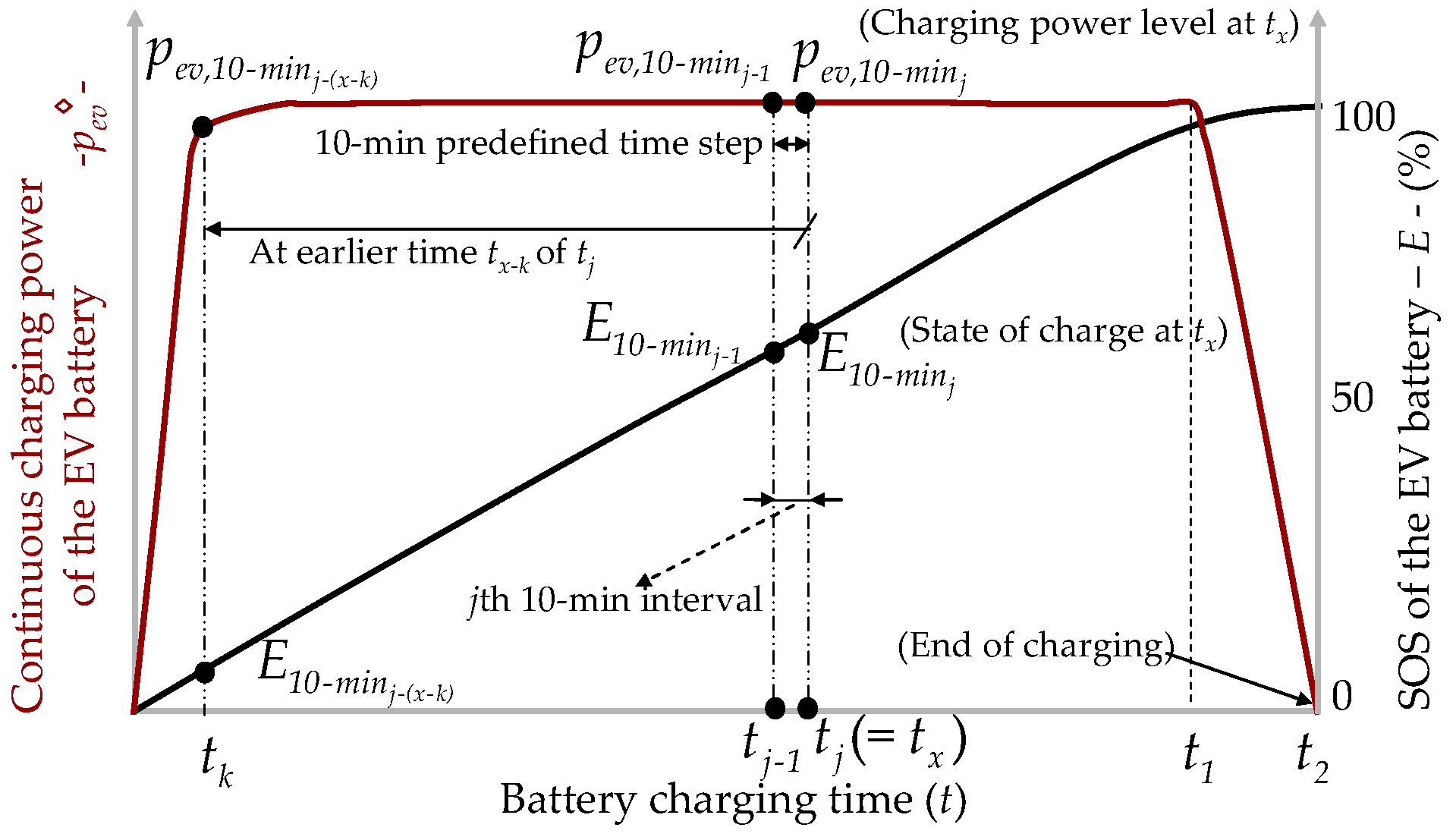
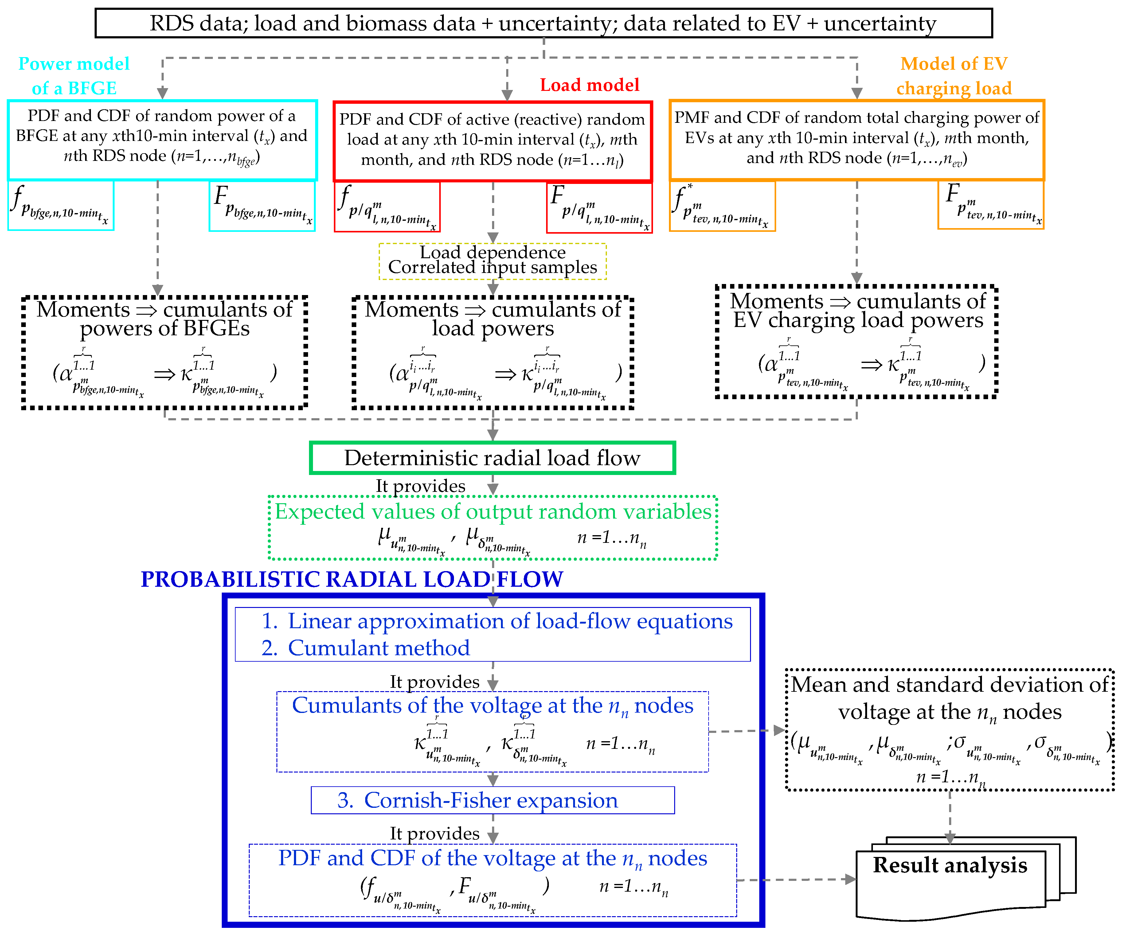
4. Proposed Analytical Technique (PAT) to Assess the Impact of BFGEs and EVs on RDSs

Figure 2 shows a flowchart of the PAT to assess the impact of BFGEs and EVs on RDSs. The steps of this technique are presented below. Firstly, distributions (PDF or PMF and CDF) of RSD input random variables at any xth 10-min interval of the day, mth month, and nth RDS node are obtained (Section 3). Then, correlated input samples of node loads are generated (Section 3.2.1). These samples are used to determine the moments and cumulants of these random inputs (Section 2). For EV charging loads and powers of BFGEs, their distributions are used to directly determine moments and then cumulants (Section 2). Subsequently, a deterministic radial load flow (Section 4.1) determines the expected values of the output random variables. Taking the cumulants of input random variables into account, the probabilistic radial load flow in Section 4.2 provides the PDF and the CDF of the nodal voltage angle and magnitude at any xth 10-min interval $(t_x)$, mth month, and nth RDS node $(f_{\mathit{u}/{\mathbf{\delta }}_{{}_{\mathit{n},10-\mathit{m}\mathit{i}{\mathit{n}}_{{\mathit{t}}_{\mathit{x}}}}}^{\mathit{m}}},F_{\mathit{u}/{\mathbf{\delta }}_{{}_{\mathit{n},10-\mathit{m}\mathit{i}{\mathit{n}}_{{\mathit{t}}_{\mathit{x}}}}}^{\mathit{m}}})$.

4.1. Deterministic Radial Load Flow

The exact equations of the non-linear load-flow for a power system with BFGEs, EV charging loads, and node loads can be mathematically described by [64]:

$$\begin{array}{ll}{p}_n=p_{g,n}+p_{bfge,n}-p_{l,n}-p_{tev,n}& =u_n{\displaystyle \sum _{j=1}^{n_n}\left[u_j\left(g_{nj}\cos {\delta }_{nj}+b_{nj}sin{\delta }_{nj}\right)\right]};\\ q_n=q_{g,n}+q_{bfge,n}-q_{l,n}& =u_n{\displaystyle \sum _{j=1}^{n_n}\left[u_j\left(g_{nj}sin{\delta }_{nj}-b_{nj}\cos {\delta }_{nj}\right)\right]};n=1,\dots ,n_n\end{array}$$

(14)

The Newton-Raphson algorithm applied to Equation (14) at any xth 10-min interval and mth month provides the expected values of output random variables $({\mu }_{{\mathit{u}}_{\mathit{n},10-\mathit{m}\mathit{i}{\mathit{n}}_{{\mathit{t}}_{\mathit{x}}}}^{\mathit{m}}},{\mu }_{{\mathbf{\delta }}_{\mathit{n},10-\mathit{m}\mathit{i}{\mathit{n}}_{{\mathit{t}}_{\mathit{x}}}}^{\mathit{m}}})$ from the expected input values (see Figure 2).

4.2. Probabilistic Radial Load Flow

In order to account for the stochastic nature of uncertainties associated with input variables in an RDS with BFGEs, EV charging loads, and node loads, these variables are considered as random variables. Although the MCS is the simpler probabilistic approach because it directly uses many deterministic radial load flows, our proposal is based on an analytical technique that is computationally more effective than the MCS [41]. This first involves the linear approximation of load-flow Equation (14) (Figure 2). In a subsequent step, the cumulant method [42] is applied to determine the cumulants of output variables. Finally, the PDF and CDF of the output variables are approximated from known output cumulants by using the Cornish-Fisher expansion [54].

4.2.1. Linear Approximation of Load-Flow Equations

The linear approximation of the load-flow Equation (14) is used to obtain the output random variables of an RDS as a linear combination (weighted sum) of the RDS random inputs. The linearization process is made around the solution point of the deterministic load flow in Section 4.1, namely, the expected values of output random variables.

To illustrate this technique, let A and B be two random variables which, at some stage of the computations, are multiplied to give a third random variable $(\mathit{Y}=\mathit{A}\cdot \mathit{B}).$ If the deviations of A and B are represented around their expected values $({\mu }_A,{\mu }_B)$, they are $\Delta \mathit{A}$ and $\Delta \mathit{B}$, respectively. The following can thus be assumed:

$$\mathit{A}\approx {\mu }_A+\Delta \mathit{A};\mathit{B}\approx {\mu }_B+\Delta \mathit{B}$$

(15)

When second-order terms are not considered, Equation (16) is obtained:

$$\mathit{Y}\approx {\mu }_B\cdot \Delta \mathit{A}+{\mu }_A\cdot \Delta \mathit{B}+{\mu }_A{\mu }_B={\mu }_B\cdot \mathit{A}+{\mu }_A\cdot \mathit{B}-{\mu }_A{\mu }_B$$

(16)

This approximation is accurate for cases where the dispersion of the random variables is limited around the mean value.

This technique can be applied to voltage magnitudes and angles in Equation (14). For the angles in Equation (14), Maclaurin’s series are firstly used in sin and cos functions, and then the linear approximation is applied [18]. Therefore, it can be assumed that:

$$\begin{array}{l}{u}_n{u}_{j}sin{\delta }_{nj}\approx a_{nj}^{\prime }+b_{nj}^{\prime }{\delta }_{nj}+c_{nj}^{\prime }{u}_n+d_{nj}^{\prime }{u}_j(e.g.a_{nj}^{\prime }=2{\mu }_{u_n}{\mu }_{u_j}{\mu }_{{\delta }_{nj}}(-1+{\mu }_{{\delta }_{nj}}^2/3))\\ u_n{u}_{j}cos{\delta }_{nj}\approx a_{nj}^{″}+b_{nj}^{″}{\delta }_{nj}+c_{nj}^{″}{u}_n+d_{nj}^{″}{u}_j\end{array}$$

(17)

When these approximations are substituted in Equation (14), the following can be obtained:

$$\begin{array}{ll}{p}_{g,n}+p_{bfge,n}-p_{l,n}-p_{tev,n}& ={\displaystyle \sum _{j=1}^{n_n}\left(e_{nj}^{\prime }+f_{nj}^{\prime }{\delta }_n-f_{nj}^{\prime }{\delta }_j+g_{nj}^{\prime }{u}_n+h_{nj}^{\prime }{u}_j\right)}\\ q_{g,n}+q_{bfge,n}-q_{l,n}& ={\displaystyle \sum _{j=1}^{n_n}\left(e_{nj}^{″}+f_{nj}^{″}{\delta }_n-f_{nj}^{″}{\delta }_j+g_{nj}^{″}{u}_n+h_{nj}^{″}{u}_j\right)}\end{array}$$

(18)

Coefficients $e_{nj}^{\prime },e_{nj}^{″},f_{nj}^{\prime },f_{nj}^{″},g_{nj}^{\prime },g_{nj}^{″},h_{nj}^{\prime },\mathrm{and} h_{nj}^{″}$ are computed from RDS parameters and the expected values of the output random variables in the RDS.

4.2.2. Cumulants Method

The convolution of the random variables in the equations in (18) can be substituted by the summation of their cumulants, which greatly reduces the computational cost [18]. Thus, the cumulant method [42] (Figure 2) is used to determine the cumulants of the output random variables in an RDS, i.e., nodal voltage angles and magnitudes (${\kappa }_{\mathit{u}/{\mathbf{\delta }}_{\mathit{n},10-\mathit{m}\mathit{i}{\mathit{n}}_{{\mathit{t}}_{\mathit{x}}}}^{\mathit{m}}}^{\underset{1\dots 1}{\overset{r}{\leftrightarrow }}}$). This means that it is necessary to solve the system of Equation (18) for each cumulant order of the input random variables, i.e., node loads, BFGE powers, and EV charging powers.

4.2.3. Cornish-Fisher Expansion

The Cornish-Fisher expansion [54] permits the approximation to the distribution function of a random variable from its cumulants (Figure 2). The expansion is based on quantile estimation (inverse function of CDF).

5. Test System Description

5.1. RSD, BFGE, and Node Load Data

The analytical technique presented was applied to the study case of the ENDE 100 RDS [65] (Figure 3). The choice of this RDS was the result of the analysis of multiple RDSs to capture the effects of their diversity. This rural RDS, which is located near the city of Úbeda (Jaén, Spain), has 100 nodes, 99 lines and 24 laterals. The total area covered is over 375.3 km² with 43% devoted to olive groves [66]. Úbeda has become one of the largest olive oil producers and bottlers in the province of Jaén [9].

The allocation and sizing of BFGEs in the ENDE 100 RDS are shown in Figure 3, i.e., 13 BFGEs with a 9.52% penetration and a BFGE capacity factor of around 0.95. Those nodes and rated powers were the result of the optimization process in [65]. This does not mean that in this study these connections were the optimal ones, only that they were feasible for this work. The resulting electric power of the biomass amount in the RDS area (about 4.5 MW [9]) was larger than the set power in the BFGEs under investigation. The main technical parameters of the BFGEs are shown in [12].

The statistical and non-statistical data concerning the amount of biomass available for each nth RDS node in the ENDE 100 RDS area, i.e., A_n, τ_n, D_n, were obtained from databases and geographic information systems [67,68,69,70,71]. The statistical data of the higher HV of the biomass was found in [51,52]. References [10,72,73] provide more information on BFGE global efficiency which ranges between 0.16 and 0.25 p.u. Our study used the 0.20-p.u. value.

The synchronous generator coupled to the BFGEs may or may not be able to control the node voltage. When this control was applied, the voltage set-point was the resulting voltage of the base case, i.e., voltage without EVs or BFGEs. Additionally, this set-point was restricted by the lower/upper voltage threshold in regulation [40] (the ±7%-threshold). The results of the reactive power were not necessary for the intended purpose. Data for real and reactive load profiles were collected at each node in 10-min intervals by using smart meters over a five-year time period. The load correlation matrix [58,59] was obtained from synchronous 10-min measurements.

5.2. EV Data

The number of EVs distributed at each RDS node was based on the average Spanish household power demand (approximately 0.897 kW/year [74,75]) and the average number of vehicles per household (1.87 in 2014 in Spain [74]). These two statistics made it possible to approximately calculate the number of EVs in nodes from the annual average active power of each node. This research was based on a 30%-penetration level for EVs according to EPRI [76]. Mode #2 was selected (Table 1) since mode #1 was found to be too slow to ensure EV charging in short-time periods, and mode #3 required a higher power level.

The annual mean and standard deviations of the daily driving distance d by vehicles in Spain were equal to 35 and 9.6 km, respectively [74,77]. All EVs were assumed to have a typical battery pack of 25-kWh and an all-electric range of up to 128.7 km (d_r).

The modelling of the charging start time of EVs, i.e., PDF for each nth load node was roughly bell-shaped. Accordingly, the resulting normal distributions for the Spanish pattern had a mean in the interval 0:00–1:30 a.m. and a standard deviation of 4.1–6.2 h depending on the mth month of the year [17,74]. On the other hand, the PDF of the random variable, parking duration at home was also determined from data for Spain [74].

6. Simulation Results

The PAT was implemented in MATLAB (The MathWorks, Inc., Natick, MA, USA) and tested in the ENDE 100 RDS. The results focused on node 97 (critical node for voltage regulation) and node 74 (internal node without BFGEs). All results are given in p.u., and the selected power base and voltage base were 100 MVA and 20 kV, respectively. A computer with an Intel^® Core^TM i7-7700 processor 3.60 GHz CPU and 8 GB RAM was used.

6.1. Case Study

Since the main objective of this study was to accurately assess the BFGE and EV impact on voltage constraint fulfilment [39,40] in RDSs, various scenarios were planned: (i) scenario #1 (base case without EVs or BFGEs); (ii) scenario #2 (with EVs and without BFGEs); (iii) scenario #3 (without EVs and with BFGEs [no voltage control]); (iv) scenario #4 (without EVs and with BFGEs [voltage control]); (v) scenario #5 (with EVs and with BFGEs [no voltage control]); (vi) scenario #6 (with EVs and with BFGEs [voltage control]). All scenarios were analyzed during a full working day in January and July on the basis of 10-min intervals. However, for the sake of completeness and because of space limitations, we focused on the 10-min interval around 00:00 h and 08:00 h, in order to show the effects of the time variability of the node load and EV charging load.

6.2. Results

6.2.1. PDF of the Input Random Variables in the RDS

Statistical data of biomass, EVs and RDS node loads were used to calculate, according to Section 3, the PDFs of the BFGE powers, node load powers and EV charging powers in the RDS nodes for each 10-min interval throughout the days of the year. As a representative example of particular day, month and node, Figure 4 shows the PDFs of the EV charging power and node load power at node 97 for a winter working day (January). These represent 144 PDFs for a 24-h duration. The EVs mostly charged at off-peak time when the electricity price was cheaper. Node load power was greater during the evening than in the daytime. This was evident in the flatter distribution towards the evening and a higher peak close to zero for hours of low power consumption.

Figure 5 focuses on the PDFs of the BFGE power and EV charging power at node 97 for two 10-min intervals (around 00:00 h and 08:00 h) for a working day in January and July. The EV charging power was time-dependent, i.e., distribution parameters depended on the time of day, day of week, and month. The PDFs of this EV charging power fit a normal distribution. In contrast, the PDF of the BFGE power did not follow any known distribution. Cumulants of these distributions are shown in

Table 2. Cumulants of BFGE power and EV charging power at node 97 during a working day (around 00:00 h and 08:00 h).

BFGE Power $\mathit{y}={\mathit{p}}_{\mathit{b}\mathit{f}\mathit{g}\mathit{e},97,10-\mathit{m}\mathit{i}{\mathit{n}}_{23\text{:}55-00\text{:}05\mathbf{or}07\text{:}55-08\text{:}05}}^{1\mathbf{or}7}$		EV Charging Power $\mathit{y}={\mathit{p}}_{\mathit{t}\mathit{e}\mathit{v},97,10-\mathit{m}\mathit{i}{\mathit{n}}_{23\text{:}55-00\text{:}05\mathbf{or}07\text{:}55\text{:}08\text{:}05}}^{1\mathbf{or}7}$
Cumulants	January or July	January (23:55–00:05)	January (07:55–08:05)	July (23:55–00:05)	July (07:55–08:05)
${\kappa }_y^1$	0.519 × 10−3	0.620 × 10−3	0.269 × 10−3	0.431 × 10−3	0.185 × 10−3
${\kappa }_y^{11}$	9.35 × 10−8	10.5322 × 10−9	5.5852 × 10−9	7.2637 × 10−9	2.9209 × 10−9
${\kappa }_y^{111}$	3.33 × 10−13	-	-	-	-
${\kappa }_y^{1111}$	1.47 × 10−16	-	-	-	-
${\kappa }_y^{11111}$	3.84 × 10−15	-	-	-	-
${\kappa }_y^{111111}$	2.39 × 10−12	-	-	-	-
${\kappa }_y^{1111111}$	−2.97 × 10−8	-	-	-	-

. The first and second cumulants are the mean and variance.

6.2.2. Assessment of the Technical Impact of BFGEs and EVs on RDSs

Firstly, the assessment presents a general overview of the technical impact on the voltage profile for the all of the nodes in the RDS. Accordingly, Figure 6 and Figure 7 present the results of the expected value and standard deviation of the 10-min voltage magnitude, around 00:00 h and 08:00 h, respectively, for each RDS node in different scenarios and months.

Various conclusions can be derived from the results in Figure 6 and Figure 7. Initially, some node voltages in scenario #1 (base case) in July (around 00:00 h) were lower than the 7%-voltage threshold in the Spanish regulation [40]. This revealed that actions would be performed in the RDS to improve certain voltages. When the EV charging loads were connected to the RDS (scenario #2), the node voltages were even lower than in scenario #1. This caused an unacceptable condition for some nodes both in January (around 08:00 h) and July (around 00:00 h and 08:00 h). Accordingly, BFGEs were connected to increase undesirable voltages. When synchronous generators coupled to BFGEs had no node voltage control, the voltage in problematic nodes (72 to 99) increased noticeably in both January and July. The new voltage profile in nodes was smoother, and all voltages remained within standard limits. However, when this node voltage control was enabled, the node voltages increased to a lesser extent and were close to voltages in the base case.

As can be observed in Figure 6 and Figure 7, the standard deviation increased when new loads or generators were connected to the RDS. This was particularly evident in the EV single condition (scenario #3) in comparison to when EVs and BFGEs were combined (scenario #5). This was because of the introduction of new variables in the RDS (BFGEs), with an increased uncertainty, which originated greater uncertainty in the output variables (i.e., node voltages). This effect was clearly evident when the synchronous generators coupled to BFGEs had no voltage control because the standard deviation of output variables associated with BFGE power was much higher than that of the EV charging power. However, the null or very low standard deviation associated with BFGE power when voltage control was enabled originated a very low deviation in the combined scenario (scenario #6).

Figure 8 and Figure 9 focus on the PDFs of the voltage magnitude at nodes 74 and 97, respectively, for different scenarios and two 10-min intervals (around 00:00 h and 08:00 h) during a working day in January and July. These figures highlight the higher dispersion associated with BFGE power (without node voltage control, scenario #3) in relation to EV charging power (scenario #2). Furthermore, the combined impact (scenario #5) averaged the dispersion of the output variable (i.e., the node voltage). The node voltage control in synchronous generators coupled to BFGEs had the advantage of greatly decreasing the dispersion in the resulting distributions for single scenarios (scenario #4) or even in combined scenarios (scenario #5) throughout all of the RDS nodes. Nodes without standard deviation are those where the voltage was fixed by voltage control.

The distribution functions of node voltages in each scenario, day, and month can be used to determine the probability of voltage threshold violation [78]. As an example, Figure 10 shows these distributions for nodes 74 and 97 during a working day in July for scenario #2. Taking into account the ±7 threshold in [40], the probability of voltage threshold violation for nodes 70 to 97 (critical nodes for voltage regulation) during a working day in July for scenario #2 are shown in Figure 11a. Despite the fact that Figure 6a shows the mean voltage value at each RDS node, this value cannot be compared with the standard limit [40]. For example, the expected voltage value at node 72 during a working day in July for scenario #2 (around 00:00 h) was 0.932 p.u. (see Figure 6a), within standard limits. However, the relevant voltage violation probability was not 0 (see Figure 11a). The voltage dispersion originated a voltage violation probability of 0.072.

The same voltage violation study when the combined impact of BFGEs and EVs was considered (scenarios #4 and #6, Figure 11b) revealed a significant decrease in the voltage violation probability for all of the nodes in comparison to the single EV impact, Figure 11a. This result emphasized how the BFGE units in the test RDS with EVs noticeably helped to keep node voltages within regulation limits. This outcome should be emphasized since the connection of BFGE units in RDSs could generate reverse flow and thus cause voltage problems.

6.2.3. Proposed Analytical Technique (PAT) versus MCS

In order to demonstrate the accuracy of the PAT (at any xth 10-min interval), its results were compared with those of the MCS for 10,000 trials, which was used as a reference. This assessment was carried out, based on the individual relative error of the first seven moments for each RDS output random variable. In particular, this error in the voltage magnitude at any nth node, xth 10-min interval of the day ($t_x$), and mth month is given by [37]:

$${\epsilon }_{{\alpha }_{u_{n,10-mi{n}_{t_x}}^m}^{\underset{1\dots 1}{\overset{r}{\leftrightarrow }}}}=\frac{100\cdot \left|{\alpha }_{{\mathit{u}}_{n,10-mi{n}_{t_x}}^m}^{\underset{1\dots 1}{\overset{r}{\leftrightarrow }},\mathbf{PAT}}-{\alpha }_{{\mathit{u}}_{n,10-mi{n}_{t_x}}^m}^{\underset{1\dots 1}{\overset{r}{\leftrightarrow }},\mathbf{MCS}}\right|}{{\alpha }_{{\mathit{u}}_{n,10-mi{n}_{t_x}}^m}^{\underset{1\dots 1}{\overset{r}{\leftrightarrow }},\mathbf{MCS}}}$$

(19)

As an example of a 10-min interval, the values in

Table 3. Individual relative error of the first seven moments of the 97-node voltage magnitude (10-min interval around 00:00 h during a working day of July).

Scenarios/Error (%)	${\mathit{\epsilon }}_{{\mathit{\alpha }}_{{\mathit{u}}_{97,10-\mathit{m}\mathit{i}{\mathit{n}}_{23\text{:}55-00\text{:}05}}^7}^1}$	${\mathit{\epsilon }}_{{\mathit{\alpha }}_{{\mathit{u}}_{{97,10-\mathbf{min}}_{23\text{:}55-00\text{:}05}}^7}^{11}}$	${\mathit{\epsilon }}_{{\mathit{\alpha }}_{{\mathit{u}}_{{97,10-\mathbf{min}}_{23\text{:}55-00\text{:}05}}^7}^{111}}$	${\mathit{\epsilon }}_{{\mathit{\alpha }}_{{\mathit{u}}_{{97,10-\mathbf{min}}_{23\text{:}55-00\text{:}05}}^7}^{1111}}$	${\mathit{\epsilon }}_{{\mathit{\alpha }}_{{\mathit{u}}_{{97,10-\mathbf{min}}_{23\text{:}55-00\text{:}05}}^7}^{11111}}$	${\mathit{\epsilon }}_{{\mathit{\alpha }}_{{\mathit{u}}_{{97,10-\mathbf{min}}_{23\text{:}55-00\text{:}05}}^7}^{111111}}$	${\mathit{\epsilon }}_{{\mathit{\alpha }}_{{\mathit{u}}_{{97,10-\mathbf{min}}_{23\text{:}55-00\text{:}05}}^7}^{1111111}}$
#1	0.053	1.173	1.651	2.299	2.289	1.259	3.458
#2	0.062	1.462	2.178	2.756	2.545	1.598	4.698
#3	0.072	1.627	2.325	3.168	2.659	1.659	5.129
#5	0.081	1.911	2.653	3.568	3.056	2.024	6.225

show that the expected values and standard deviations (first two moments) could be accurately estimated using the PAT for the most critical node (node #97) and for several scenarios. The higher moments were nearly accurate. In other words, the PAT had accuracy levels similar to the MCS for calculating the statistics of voltage magnitude. Moreover,

Table 4. Run time comparison (10-min interval around 00:00 h during a working day in July).

Scenarios		#1	#2	#3	#4	#5	#6
Computation time (s)	PAT	0.48	0.54	0.60	0.72	0.77	0.91
	MCS	508.86	641.99	735.94	874.12	1002.60	1156.62

illustrates that the computation time required by the PAT was considerably less than that of the MCS. In addition, the same accuracy was obtained.

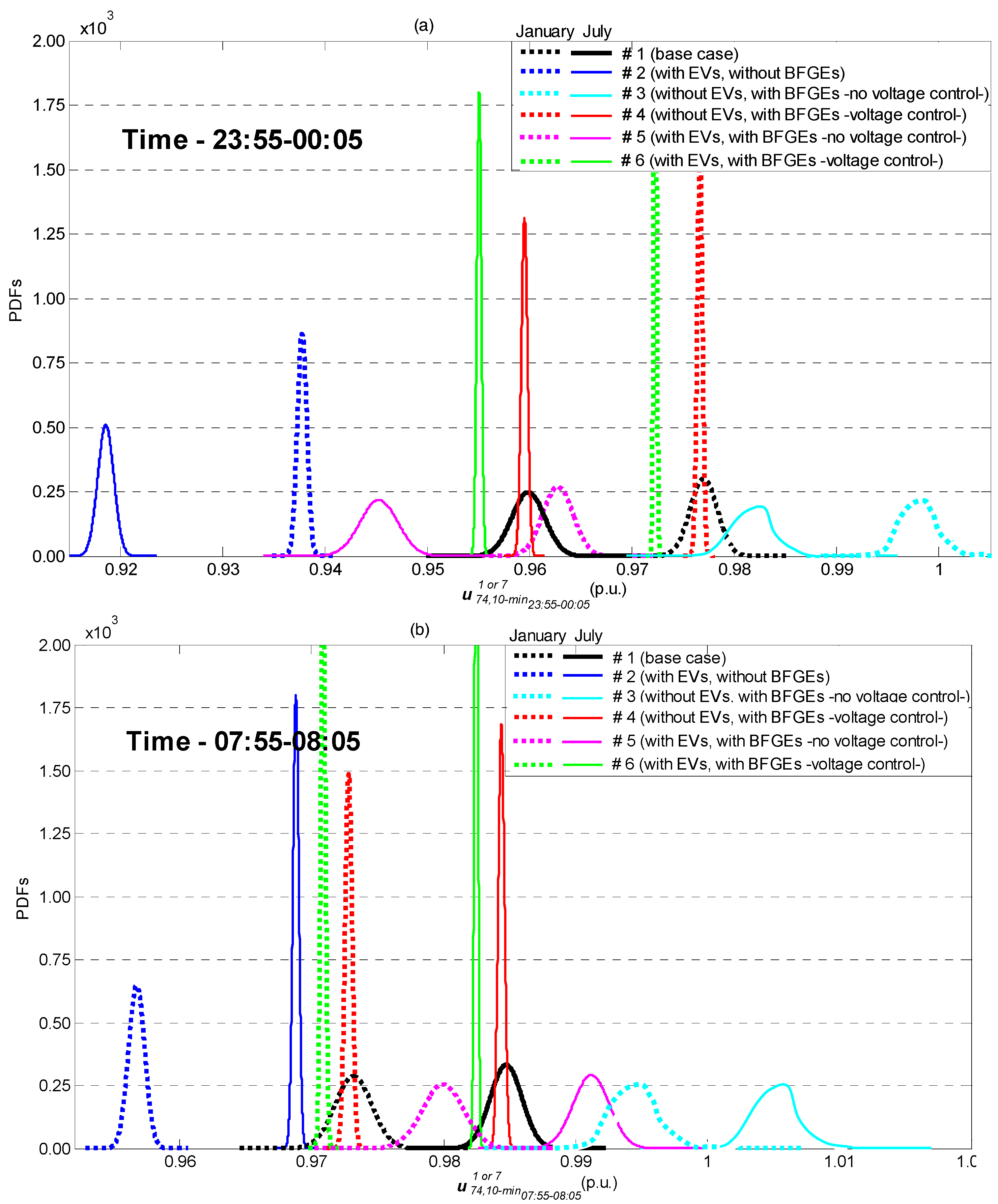
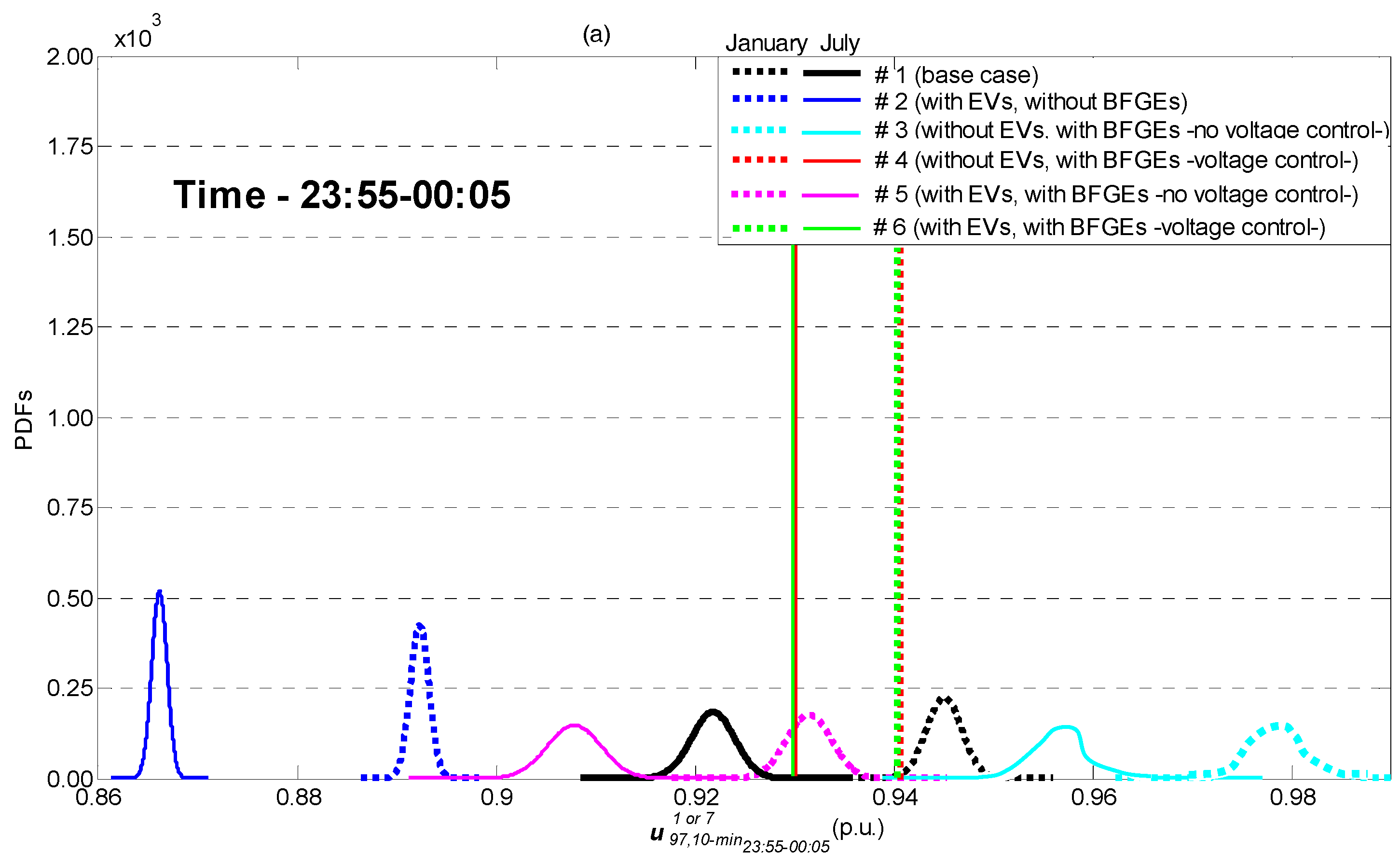
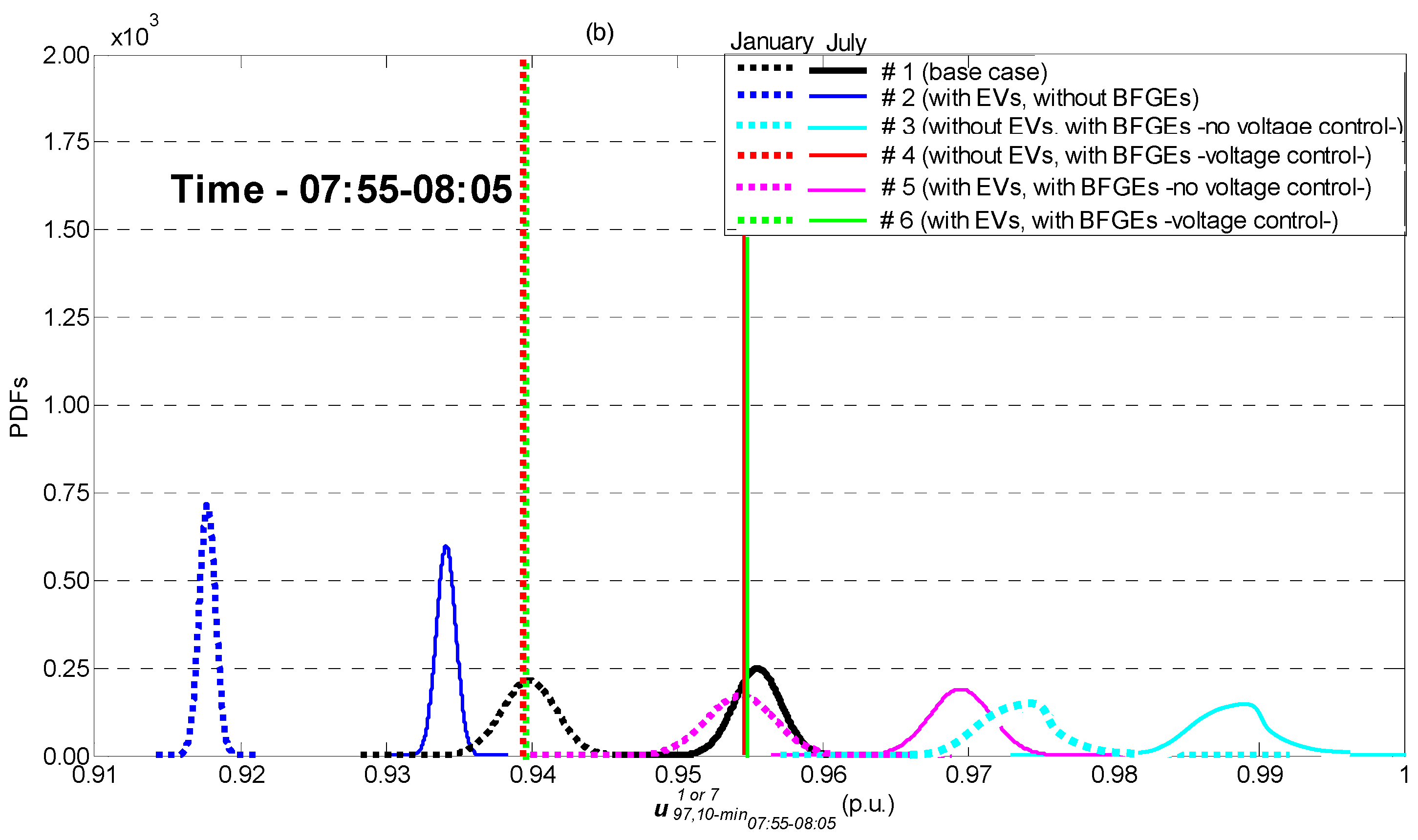
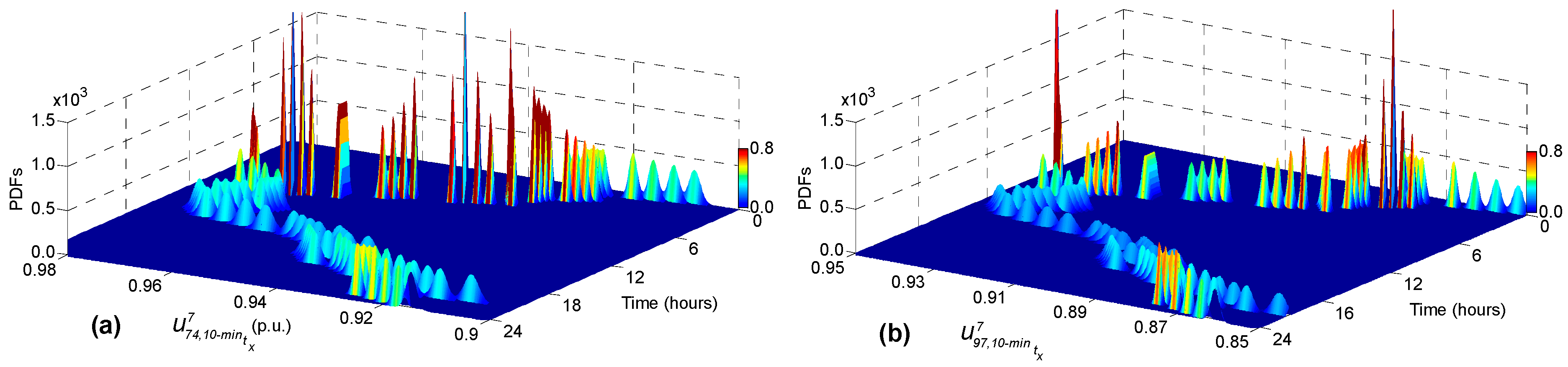
7. Conclusions and Discussion

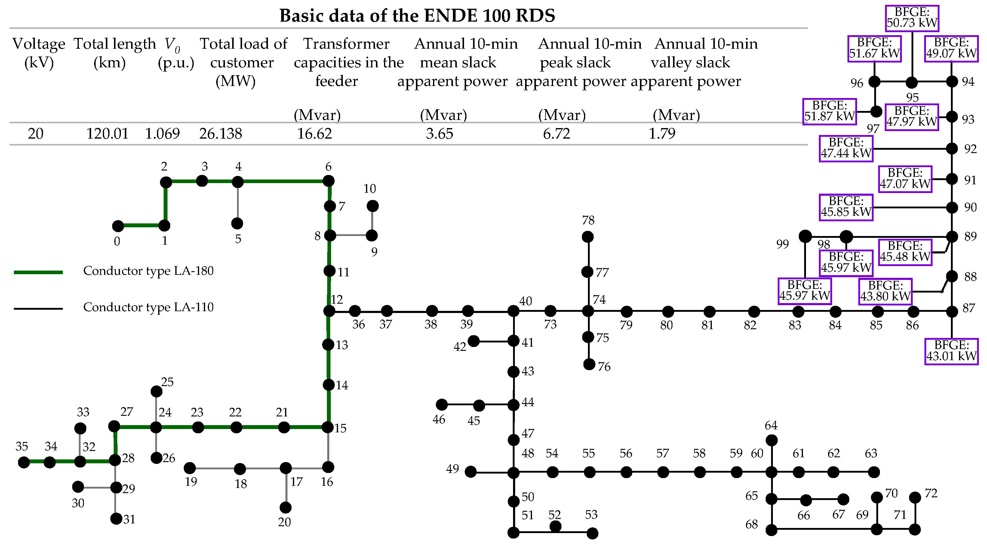
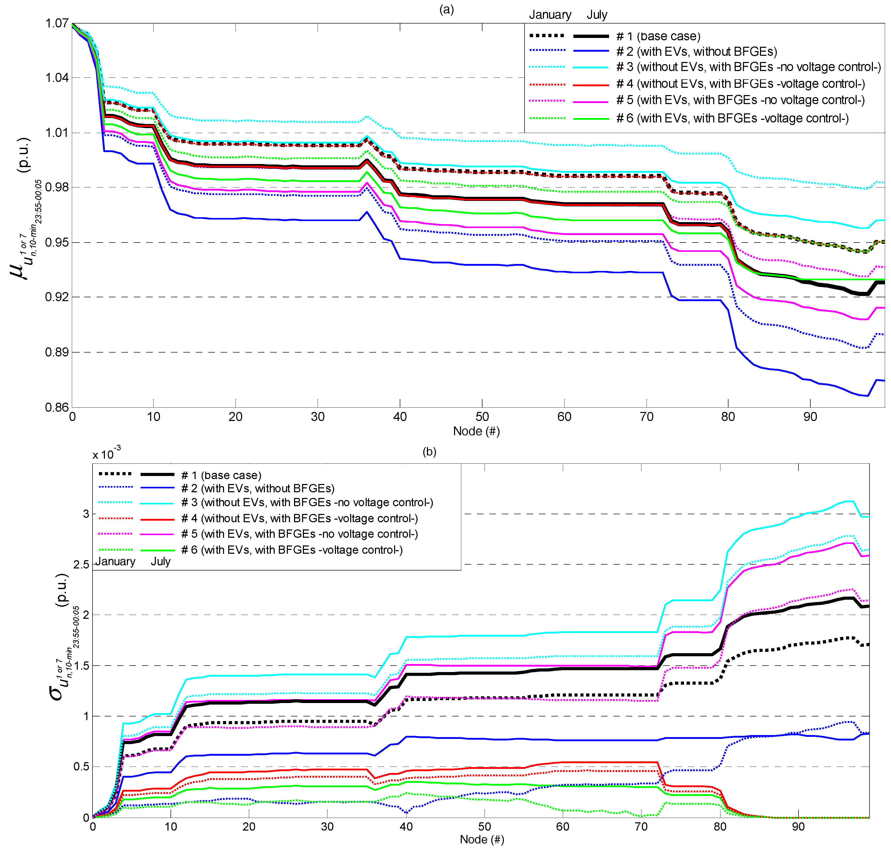
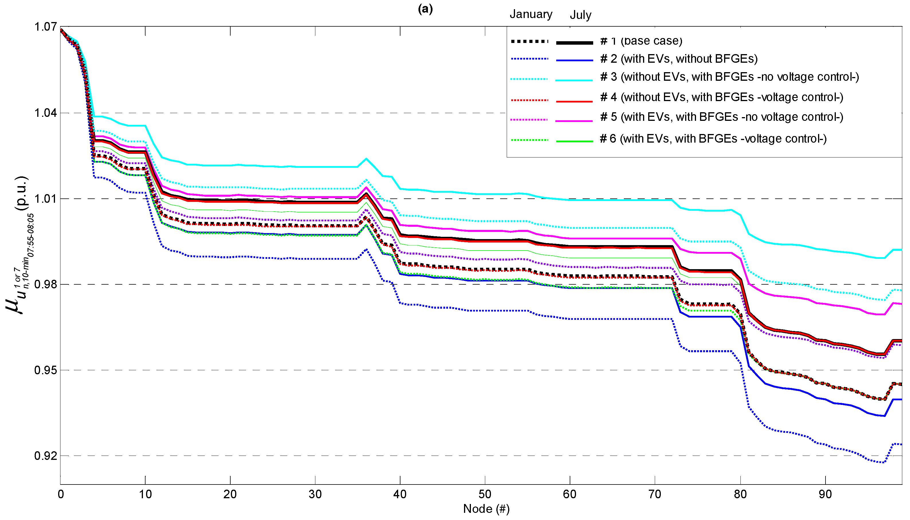
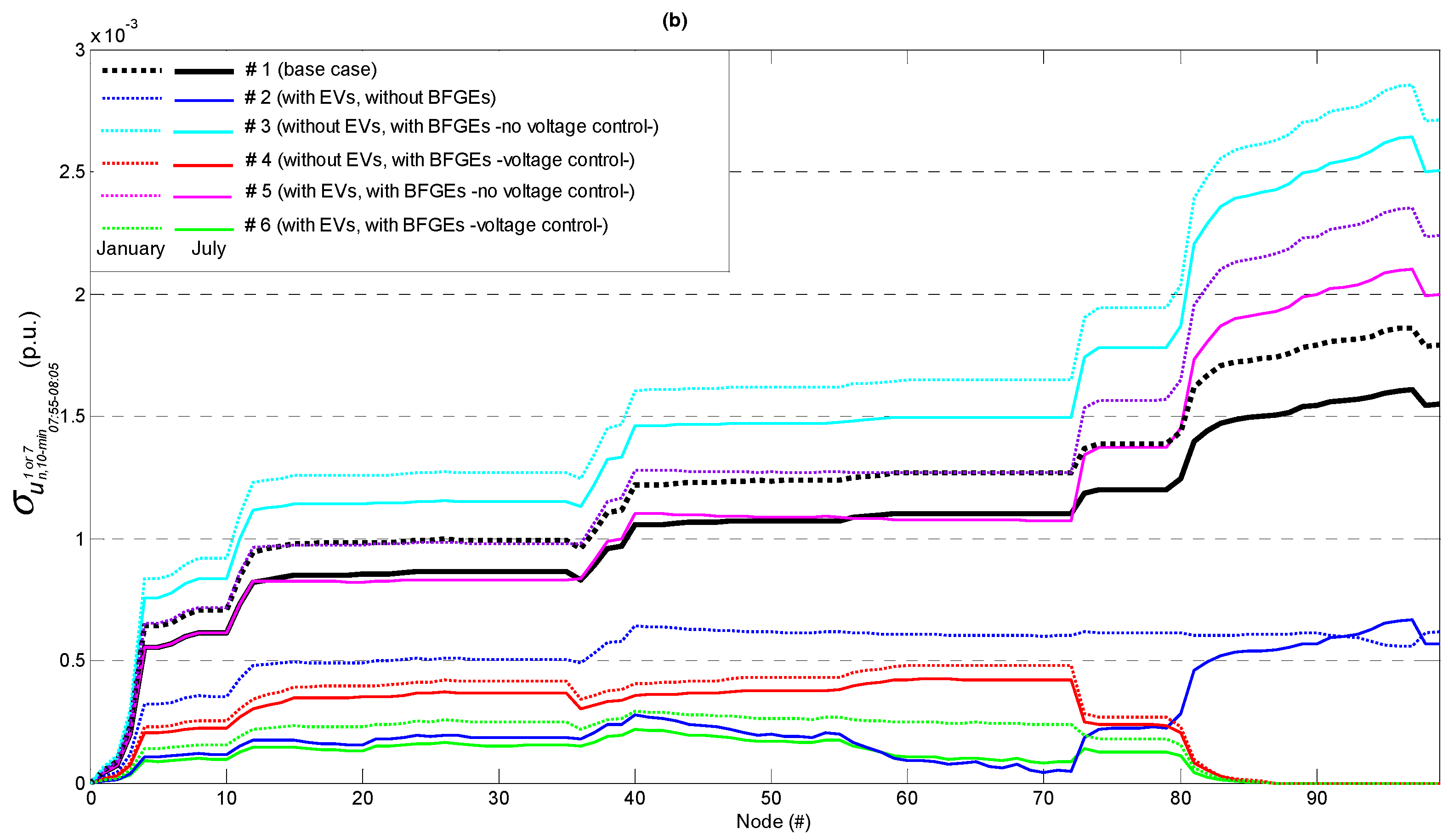
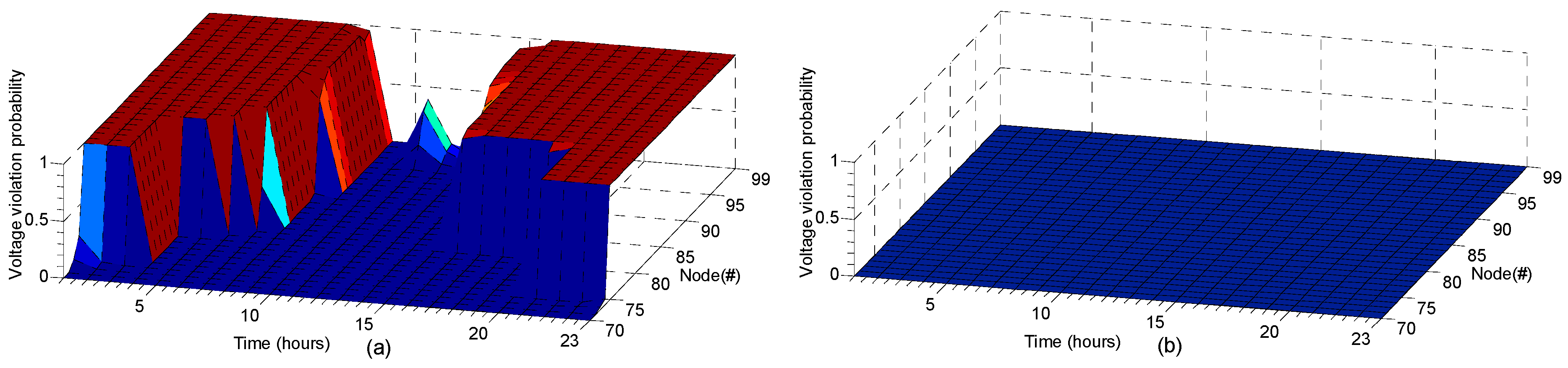
The paper has presented an analytical technique which was tested on an operating ENDE 100 RDS in Spain [65]. This technique was used to accurately assess the fulfilment of voltage constraints in the overall RDS with uncertainty in the loads (node load and EV charging load) and generations (BFGEs). The MCS was applied to highlight the accuracy of the results obtained with the PAT. Moreover, the PAT achieved a high computational cost reduction in comparison to the MCS.

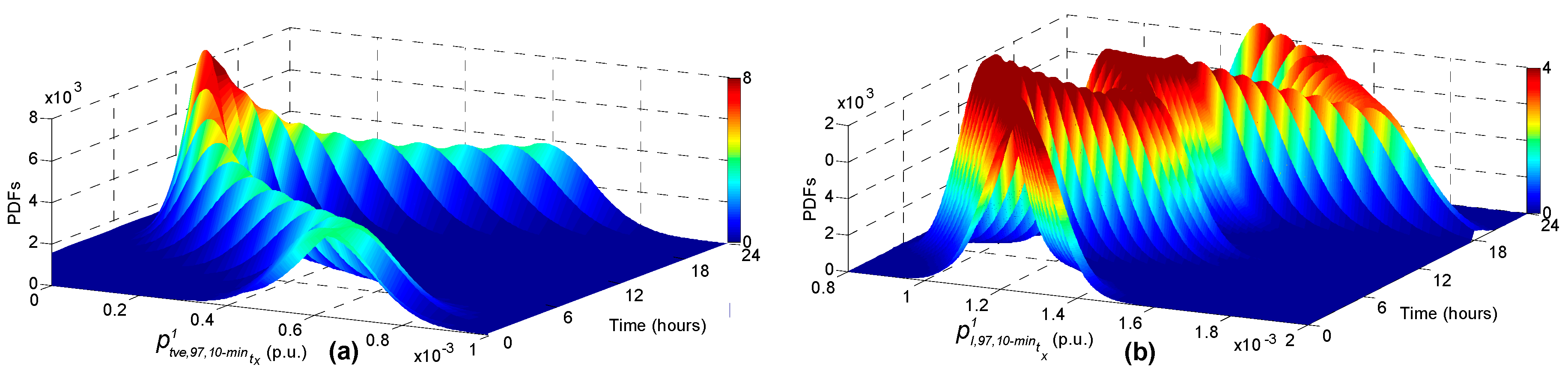
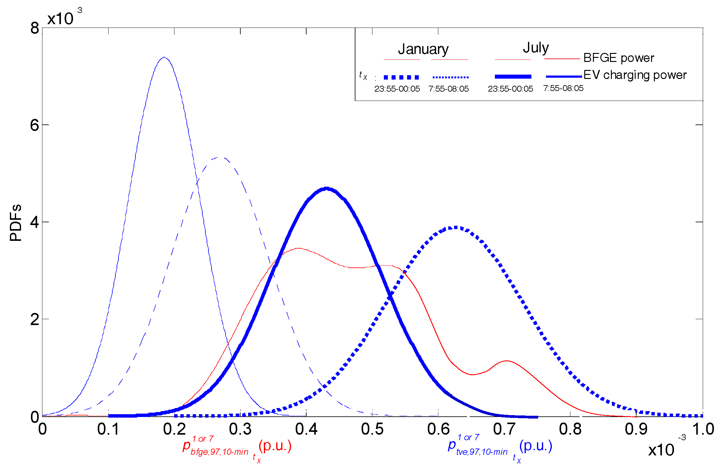
This study required the use of a stochastic model of BFGE power and EV charging loads suitable for probabilistic studies. The availability of a large amount of statistical data for the model in the operating RDS provided valuable insights and led to interesting outcomes. As a result, this research demonstrated that the combined impact of BFGEs and EVs on the test RDS differed considerably from the individual impact. In fact, the results showed that it generally improved. Accordingly, the voltage violation probability in the RDS nodes due to EVs decreased significantly when BFGEs were connected to the RDS. Furthermore, the lower dispersion in distributions in some combined scenarios meant that this fulfilment could be absolutely guaranteed.

More specifically, results revealed substantial relative uncertainties for the HV of the biomass (61–138% of predicted means) with even larger uncertainties for the amount of biomass available (37–153%) in the power model of a BFGE. These results suggest that biomass uncertainty models are extremely relevant, something that has not been previously reported by the literature.

This new approach provided a more accurate assessment than other evaluations, based on a simple deterministic vision. In this way, the PAT could provide useful insights for RDS design and operation and offers a better understanding of the combined impact of renewable power sources.

In the future, more EV charging loads will be connected to the RDSs, and therefore actions will be performed in the RDSs to maintain the voltage constraint fulfilment. One of these actions could be the connection of BFGEs, as shown in this research, without changes in the RDS structure.

References

1. Alley, R.; Berntsen, T.; Bindoff, N.L.; Chen, Z.; Chidthaisong, A.; Friedlingstein, P.; Gregory, J.; Hegerl, G.; Heimann, M.; Hewitson, B.; et al. Climate Change 2007: The Physical Science Basis, Summary for Policymakers, Intergovernmental Panel on Climate Change. 2007. Available online: http://www.ipcc.ch (accessed on 11 June 2017).
2. International Energy Agency. Available online: https://www.iea.org (accessed on 10 June 2017).
3. The WorldWatch Institute. The World State of the World. Innovations for a Sustainable Economy. Available online: https://www.worldwatch.org (accessed on 13 June 2017).
4. Rezaee, S.; Farjah, E.; Khorramdel, B. Probabilistic analysis of plug-in electric vehicles impact on electrical grid through homes and parking lots. IEEE Trans. Sustain. Energy 2013, 4, 1024–1033. [Google Scholar] [CrossRef]
5. Directive 2009/28/EC of the European Parliament and of the Council of 23 April 2009 on the promotion of the use of energy from renewable sources and amending and subsequently repealing Directives 2001/77/EC and 2003/30/EC. Available online: http://eur-lex.europa.eu/legal-content/EN/ALL/?uri=celex%3A32009L0028 (accessed on 2 October 2017).
6. Vargas-Moreno, J.M.; Callejón-Ferre, A.J.; Pérez-Alonso, J.; Velázquez-Martí, B. A review of the mathematical models for predicting the heating value of biomass materials. Renew. Sustain. Energy Rev. 2012, 16, 3065–3083. [Google Scholar] [CrossRef]
7. Blasi, C.D.; Tanz, V.; Lanzetta, M. A study on the production of agricultural residues in Italy. Biomass Bioenergy 1997, 12, 321–331. [Google Scholar] [CrossRef]
8. Skytte, K.; Meibom, P.; Henriksen, T.C. Electricity from biomass in the European union with or without biomass import. Biomass Bioenergy 2006, 30, 385–392. [Google Scholar] [CrossRef]
9. Vera, D.; Carabias, J.; Jurado, F.; Ruiz-Reyes, N. A Honey bee foraging approach for optimal location of a biomass power plant. Appl. Energy 2010, 87, 2119–2127. [Google Scholar] [CrossRef]
10. Vera, D.; Jurado, F.; Panopoulos, K.D.; Grammelis, P. Modelling of biomass gasifier and microturbine for the olive oil industry. Int. J. Energy Res. 2012, 36, 355–367. [Google Scholar] [CrossRef]
11. De Gennaro, B.; Notarnicola, B.; Roselli, L.; Tassielli, G. Innovative olive-growing models: An environmental and economic assessment. J. Clean. Prod. 2012, 28, 70–80. [Google Scholar] [CrossRef]
12. Ruiz-Rodriguez, F.J.; Gomez-Gonzalez, M.; Jurado, F. Optimization of radial systems with biomass fueled gas engine from a metaheuristic and probabilistic point of view. Energy Convers. Manag. 2013, 65, 343–350. [Google Scholar] [CrossRef]
13. Budzianowski, W.M. Opportunities for bioenergy in Poland: Biogas and biomass fuelled power plants. Rynek Energii 2011, 94, 138–146. [Google Scholar]
14. Sanchez-Sutil, F.; Hernandez, J.C.; Tobajas, C. Overview of electrical protection requirements for integration of a smart DC node with bidirectional electric vehicle charging stations into existing AC and DC railway grids. Electr. Power Syst. Res. 2015, 122, 104–118. [Google Scholar] [CrossRef]
15. Shabani, N.; Akhtari, S.; Sowlati, T. Value chain optimization of forest biomass for bioenergy production: A review. Renew. Sustain. Energy Rev. 2013, 23, 299–311. [Google Scholar] [CrossRef]
16. Velazquez-Martı, B.; Fernandez-Gonzalez, E.; Lopez-Cortes, I.; Salazar-Hernandez, D.M. Quantification of the residual biomass obtained from pruning of trees in Mediterranean olive groves. Biomass Bioenergy 2011, 35, 3208–3217. [Google Scholar] [CrossRef]
17. Qian, K.; Zhou, C.; Allan, M.; Yuan, Y. Modeling of load demand due to EV battery charging in distribution systems. IEEE Trans. Power Syst. 2011, 26, 802–810. [Google Scholar] [CrossRef]
18. Anders, G.J. Probability Concepts in Electric Power Systems; Wiley-Interscience: Hoboken, NJ, USA, 1990. [Google Scholar]
19. Kim, J.; Realff, M.J.; Lee, J.H. Optimal design and global sensitivity analysis of biomass supply chain networks for biofuels under uncertainty. Comput. Chem. Eng. 2011, 35, 1738–1751. [Google Scholar] [CrossRef]
20. Svensson, E.; Strömberg, A.; Patriksson, M. A model for optimization of process integration investments under uncertainty. Energy 2011, 36, 2733–2746. [Google Scholar] [CrossRef]
21. Svensson, E.; Berntsson, T. Planning future investments in emerging energy technologies for pulpmills considering different scenarios for their investment cost development. Energy 2011, 36, 6508–6519. [Google Scholar] [CrossRef]
22. Douglas, H.S.T.; Denny, K.S.N.; Raymond, R.T. Robust optimization approach for synthesis of integrated biorefineries with supply and demand uncertainties. Environ. Prog. Sustain. Energy 2012. [Google Scholar] [CrossRef]
23. Zambon, I.; Colosimo, F.; Monarca, D.; Cecchini, M.; Gallucci, F.; Proto, A.R.; Lord, R.; Colantoni, A. An innovative agro-forestry supply chain for residual biomass: Physicochemical characterisation of biochar from olive and hazelnut pellets. Energies 2016, 9, 526–537. [Google Scholar] [CrossRef] [Green Version]
24. Cano, A.; Jurado, F. Optimum location of biomass-fuelled gas turbines in an electric system. In Proceedings of the IEEE Power Engineering Society General Meeting, Montreal, QC, Canada, 18–22 June 2006; pp. 1–6. [Google Scholar]
25. Sexauer, J.M.; McBee, K.D.; Bloch, K.A. Applications of probability model to analyze the effects of electric vehicle chargers on distribution transformers. IEEE Trans. Power Syst. 2013, 28, 847–854. [Google Scholar] [CrossRef]
26. Shaaban, M.F.; Atwa, Y.M.; El-Saadany, E.F. PEVs modeling and impacts mitigation in distribution networks. IEEE Trans. Power Syst. 2013, 28, 1122–1131. [Google Scholar] [CrossRef]
27. Papadopoulos, P.; Skarvelis, S.; Grau, I.; Cipcigan, L.M.; Jenkins, N. Electric vehicles’ impact on British distribution networks. IET Electr. Syst. Transp. 2012, 2, 91–102. [Google Scholar] [CrossRef]
28. ElNozahy, M.S.; Salama, M.M.A. A comprehensive study of the impacts of PHEVS on residential distribution networks. IEEE Trans. Sustain. Energy 2014, 5, 332–342. [Google Scholar] [CrossRef]
29. Valsera-Naranjo, E.; Sumper, A.; Villafafila-Robles, R.; Martinez-Vicente, D. Probabilistic method to assess the impact of charging of EV on distribution grids. Energies 2012, 5, 1503–1531. [Google Scholar] [CrossRef] [Green Version]
30. Aljanad, A.; Mohamed, A. Impact of plug-in hybrid electric vehicle on power distribution system considering vehicle to grid technology: A review. Res. J. App. Sci. Eng. Technol. 2015, 10, 1404–1413. [Google Scholar] [CrossRef]
31. Olivella-Rosell, P.; Villafafila-Robles, R.; Sumper, A.; Bergas-Jane, J. Probabilistic agent-based model of electric vehicle charging demand to analyse the impact on distribution networks. Energies 2015, 8, 4160–4187. [Google Scholar] [CrossRef] [Green Version]
32. Leemput, N.; Geth, F.; Van Roy, J.; Delnooz, A.; Büscher, J.; Driesen, J. Impact of electric vehicle on-board single-phase charging strategies on a Flemish residential grid. IEEE Trans. Smart Grid 2014, 5, 1815–1822. [Google Scholar] [CrossRef]
33. Leou, R.-C.; Chun-Lien, S.; Chan-Nan, L. Stochastic analyses of electric vehicle charging impacts on distribution network. IEEE Trans. Power Syst. 2014, 29, 1055–1063. [Google Scholar] [CrossRef]
34. Khorramdel, B.; Khorramdel, H.; Aghaei, J.; Heidari, A.; Agelidis, V.G. Voltage security considerations in optimal operation of BEVS/PHEVS integrated microgrids. IEEE Trans. Smart Grid 2015, 6, 1575–1587. [Google Scholar] [CrossRef]
35. Zhou, B.; Littler, T.; Meegahapola, L.; Zhang, H. Power system steady-state analysis with large-scale electric vehicle integration. Energy 2016, 115, 289–302. [Google Scholar] [CrossRef]
36. Ahmadian, A.; Sedghi, M.; Aliakbar-Golkar, M.; Elkamel, A.; Fowler, M. Optimal probabilistic based storage planning in tap-changer equipped distribution network including PEVs, capacitor banks and WDGs: A case study for Iran. Energy 2016, 112, 984–997. [Google Scholar] [CrossRef]
37. Huang, H.; Chung, C.Y.; Chan, K.W.; Chen, H. Quasi-Monte Carlo based probabilistic small signal stability analysis for power systems with plug-in electric vehicle and wind power integration. IEEE Trans. Power Syst. 2013, 28, 3335–3343. [Google Scholar] [CrossRef]
38. Zhang, P.; Qian, K.; Zhou, C.; Stewart, B.G.; Hepburn, D.M. A methodology for optimization of power systems demand due to electric vehicle charging load. IEEE Trans. Power Syst. 2012, 27, 1628–1636. [Google Scholar] [CrossRef]
39. Markiewicz, H.; Klajn, A. EN Standard 50160. Voltage characteristics of electricity supplied by public distribution systems. Available online: http://www.cdtechnics.be/542-standard-en-50160-voltage-characteristics-in.pdf (accessed on 2 October 2017).
40. Spanish Royal Decree 1955/2000. Activities of transportation, distribution, commercialization, supply and procedures of authorization of electrical installations, December 27, 2000. Available online: https://www.boe.es/boe/dias/2000/12/27/pdfs/A45988-46040.pdf (accessed on 2 October 2017).
41. Ruiz-Rodriguez, F.J.; Hernandez, J.C.; Jurado, F. Probabilistic load flow for photovoltaic distributed generation using the Cornish-Fisher expansion. Electr. Power Syst. Res. 2012, 89, 129–138. [Google Scholar] [CrossRef]
42. McCullagh, P. Tensor Methods in Statistics; Chapman and Hall: London, UK, 1987. [Google Scholar]
43. Kendall, M.G.; Stuart, A. The Advanced Theory of Statistics; Charles Grin and Company Limited: London, UK, 1963; Volume 1. [Google Scholar]
44. Velazquez-Marti, B.; Fernandez-Gonzalez, E.; Callejon-Ferre, A.J.; Estornell-Cremades, J. Mechanized methods for harvesting residual biomass from Mediterranean fruit tree cultivations. Sci. Agric. 2012, 69, 180–188. [Google Scholar] [CrossRef]
45. Velazquez-Marti, B.; Fernandez-Gonzalez, E. Analysis of the process of biomass harvesting with collecting chippers fed by pick up headers in plantations of olive trees. Biosyst. Eng. 2009, 104, 184–190. [Google Scholar] [CrossRef]
46. Estornell, J.; Ruiz, L.A.; Velazquez-Marti, B.; Lopez-Cortes, I.; Salazar, D.; Fernandez-Sarria, A. Estimation of pruning biomass of olive trees using airborne discrete-return LiDAR data. Biomass Bioenergy 2015, 81, 315–321. [Google Scholar] [CrossRef]
47. Rentizelas, A.A.; Tatsiopoulos, I.P.; Tolis, A. An optimization model for multi-biomass tri-generation energy supply. Biomass Bioenergy 2009, 33, 223–233. [Google Scholar] [CrossRef] [Green Version]
48. Andalusian Energy Agency. Available online: https://www.agenciaandaluzadelaenergia.es (accessed on 24 June 2017).
49. European Project: Adaptation of renewable energy solutions for the olive oil industry (RESOLIVE). Seventh Framework Programme, 2008–2012. Available online: http://cordis.europa.eu/project/rcn/95147_es.html (accessed on 2 October 2017).
50. Sajdak, M.; Velazquez-Marti, B.; Lopez-Cortes, I. Quantitative and qualitative characteristics of biomass derived from pruning Phoenix canariensis hort. ex Chabaud. and Phoenix dactilifera L. Renew. Energy 2014, 71, 545–552. [Google Scholar] [CrossRef]
51. Jurado, F.; Ortega, M.; Cano, A.; Carpio, J. Neuro-fuzzy controller for gas turbine in biomass-based electric power plant. Electr. Power Syst. Res. 2002, 60, 123–135. [Google Scholar] [CrossRef]
52. Lopez, P.R.; González, M.G.; Reyes, N.R.; Jurado, F. Optimization of biomass fueled systems for distributed power generation using particle swarm optimization. Electr. Power Syst. Res. 2008, 78, 1448–1455. [Google Scholar] [CrossRef]
53. Springer, M.D. The Algebra of Random Variables; Wiley: New York, NY, USA, 1979. [Google Scholar]
54. Cornish, E.A.; Fisher, R.A. Moments and cumulants in the specification of distributions. Revue de l’Institut International de Statis 1937, 5, 307–322. [Google Scholar] [CrossRef]
55. Ruiz-Rodriguez, F.J.; Hernandez, J.C.; Jurado, F. Probabilistic load flow for radial distribution networks with photovoltaic generators. IET Renew. Power Gener. 2012, 6, 110–121. [Google Scholar] [CrossRef]
56. Munkhammar, J.; Widen, J.; Ryden, J. On a probability distribution model combining household power consumption, electric vehicle home-charging and photovoltaic power production. Appl. Energy 2015, 142, 135–143. [Google Scholar] [CrossRef]
57. Verbic, G.; Cañizares, C.A. Probabilistic optimal power flow in electricity markets based on a two-point estimate method. IEEE Trans. Power Syst. 2006, 21, 1883–1893. [Google Scholar] [CrossRef]
58. Li, W. Reliability Assessment of Electrical Power Systems Using Monte Carlo Methods; Springer: New York, NY, USA, 1994. [Google Scholar]
59. Li, W. Probabilistic Transmission System Planning; Wiley-IEEE Press: Hoboken, NJ, USA, 2011. [Google Scholar]
60. Papaefthymiou, G.; Kurowicka, D. Using copulas for modeling stochastic dependence in power system uncertainty analysis. IEEE Trans. Power Syst. 2009, 24, 40–49. [Google Scholar] [CrossRef]
61. Linden, D.; Reddy, T.B. Handbook of Batteries, 3rd ed.; McGraw-Hill: New York, NY, USA, 2001. [Google Scholar]
62. Madrid, C.; Argueta, J.; Smith, J. Performance Characterization-1999 Nissan Altra-EV with Lithium-Ion Battery; EDISON: Rosemead, CA, USA, 1999. [Google Scholar]
63. IEC Standard 61851–. Electric vehicle conductive charging system - General requirements, 2010. Available online: https://webstore.iec.ch/publication/6029 (accessed on 2 October 2017).
64. Grainger, J.; Stevenson, W.D. Power Systems Analysis, Electrical Engineering; McGraw-Hill International Editions: Columbus, OH, USA, 1994. [Google Scholar]
65. Hernandez, J.C.; Medina, A.; Jurado, F. Impact comparison of PV system integration into rural and urban feeders. Energy Convers. Manag. 2008, 49, 1747–1765. [Google Scholar] [CrossRef]
66. Survey on crop areas and yields: Analysis of olive groves in Spain; Ministry of Agriculture, Food and Environment: Madrid, Spain, 2013.
67. Freppaz, D.; Minciardi, R.; Robba, R.; Rovatti, M.; Sacile, M.; Taramasso, A. Optimizing forest biomass exploitation for energy supply at a regional level. Biomass Bioenergy 2004, 26, 15–26. [Google Scholar] [CrossRef]
68. Geographic Information Systems of Farming Plots. Available online: http://www.mapama.gob.es/es/cartografia-y-sig/ (accessed on 27 June 2017).
69. Geographic Information Systems of Andalusia (SIGPAC). Available online: http://www.mapama.gob.es/es/cartografia-y-sig/ (accessed on 27 June 2017).
70. Gallego, F.J.; Terrados, J.; Ruiz-Ramos, E.; Romero, I.; Martínez-Rodríguez, A. M. Model for estimating biomass potential from the olive pruning in the province of Jaén (Southern Spain). In Proceedings of the 2º Congreso Iberoamericano sobre Biorefinerias, Jaén, Spain, 17–20 April 2013; pp. 1–6. [Google Scholar]
71. Ruiz-Arias, J.A.; Terrados, J.; Perez-Higueras, P.; Pozo-Vazquez, D.; Almonacid, G. Assessment of the renewable energies potential for intensive electricity production in the province of Jaén, southern Spain. Renew. Sustain. Energy Rev. 2012, 16, 2994–3001. [Google Scholar] [CrossRef]
72. Abuadala, A.; Dincer, I.; Naterer, G.F. Exergy analysis of hydrogen production from biomass gasification. Int. J. Hydrog. Energy 2010, 35, 4981–4990. [Google Scholar] [CrossRef]
73. Toonssen, R.; Woudstra, N.; Verkooijen, A.H.M. De-centralized generation of electricity from biomass with proton exchange membrane fuel cell. J. Power Sources 2009, 194, 456–466. [Google Scholar] [CrossRef]
74. National Institute of Statistics of Spain. Available online: http://www.ine.es (accessed on 10 July 2017).
75. Eurostat. Electricity Consumption by Households. Available online: http://ec.europa.eu/eurostat (accessed on 10 July 2017).
76. Environmental assessment of plug-in hybrid electric vehicles, nationwide greenhouse gas emissions. In Technical Report; EPRI: Palo Alto, CA, USA, 2007; pp. 1–56. Available online: https://energy.gov/sites/prod/files/oeprod/DocumentsandMedia/EPRI-NRDC_PHEV_GHG_report.pdf (accessed on 2 October 2017).
77. Pasaoglu, G.; Fiorello, D.; Martino, A.; Scarcella, G.; Alemanno, A.; Zubaryeva, A.; Thiel, C. Driving and parking patterns of European car drivers—a mobility survey. In Technical Report; European Commission Joint Research Centre: Luxembourg, 2012. [Google Scholar]
78. Ruiz-Rodriguez, F.J.; Gomez-Gonzalez, M.; Jurado, F. A Method for reliability optimization of distributed generation using meta-heuristic and probabilistic techniques. Elec. Power Compon. Syst. 2015, 43, 32–43. [Google Scholar] [CrossRef]
Figure 1. Charging profile and SOC of lithium-ion batteries.
Energies 10 01536 g001
Figure 2. Flowchart of the PAT to assess the impact of BFGEs and EVs on RDSs.
Energies 10 01536 g002
Figure 3. Single-phase diagram of the ENDE 100 RDS.
Energies 10 01536 g003
Figure 4. Surface plots based on the PDFs for a working day in January at node 97. (a) EV charging power; (b) node load power.
Energies 10 01536 g004
Figure 5. PDFs of BFGE power and EV charging power at node 97 during a working day (around 00:00 h and 08:00 h).
Energies 10 01536 g005
Figure 6. 10-min voltage magnitude during a working day in January and July for each RDS node in different scenarios around 00:00 h. (a) expected value; (b) standard deviation.
Energies 10 01536 g006
Figure 7. 10-min voltage magnitude during a working day in January and July for each RDS node in different scenarios around 08:00 h. (a) expected value; (b) standard deviation.
Energies 10 01536 g007aEnergies 10 01536 g007b
Figure 8. PDFs of the 10-min voltage magnitude at node 74 in different scenarios. (a) around 00:00 h; (b) around 08:00 h.
Energies 10 01536 g008
Figure 9. PDFs of the 10-min voltage magnitude at node 97 in different scenarios. (a) around 00:00 h; (b) around 08:00 h.
Energies 10 01536 g009aEnergies 10 01536 g009b
Figure 10. Surface plots based on PDFs of 10-min voltage magnitude during a working day in July for scenario #2. (a) node 74; (b) node 97.
Energies 10 01536 g010
Figure 11. Voltage violation probability, based on regulations, for nodes 70 to 99 during a working day in July. (a) scenario #2; (b) scenarios #4 and #6.
Energies 10 01536 g011