Detailed Modelling of the Deep Decarbonisation Scenarios with Demand Response Technologies in the Heating and Cooling Sector: A Case Study for Italy

Abstract

Energy policies accompanying the transition towards a sustainable development process must be supported by technical analyses in which future energy scenarios are modeled and evaluated. This paper analyzes possible decarbonization scenarios in Italy for the year 2050. They envisage high electrification of transports and residential buildings, high use of renewable energies, and a modal shift towards public transport. The energy scenarios are evaluated using a software program, EnergyPLAN, starting from a reference model developed for the year 2014. Special attention has been given to the modeling of data that are unavailable in the literature, such as the time profile of heating and cooling demands, obtained with the degree-days method and validated by elaborating the results of the modeling of the residential building stock, this latter was dynamically simulated in TRNSYS. The results show that to obtain a significant decrease of greenhouse gas emissions and fossil fuel consumption, it is necessary not only to promote a deeper penetration of renewable sources, but also their integration with other technologies (cogeneration, trigeneration, power-to-heat systems, thermal storage, vehicle-to-grid operations). In fact, renewables technologies alone can raise some critical issues, such as excess and/or shortage of electricity production and non-sustainable exploitation of biomass.

1. Introduction

The negative effects of the energy sector on the environment, from air quality to climate changes, are commonly recognized in the scientific world as able to affect the life of future generations [1]. Therefore, in the last few years, the concept of so called “sustainable development” has hired an increasing importance among researchers and policymakers, and people have realized the need to set constrains and strategies to correct the distribution of temporal and spatial risks and costs as well as safeguard the natural capital [2].

The share of renewable energy sources (namely: hydro, solar, geothermal, wind, biomass, tidal, and wave) in gross final consumption of energy is increasing in most countries, worldwide. However, fossil fuels still cover more than 80% of the world primary energy consumption, and most scientists agree that their availability will decrease in the future. Therefore, the use of renewable energy sources will be more and more necessary to match the growing world energy demand.

In December 2015, at the Paris Conference, governments decided to put an end to the fossil fuel era, signing a general agreement to reduce greenhouse gas (GHG) emissions and to cut the negative consequences of climate change. In spite of the fact that, recently, the USA got out of the deal, the Paris Agreement is going to affect the energy policies that will be adopted and implemented in the coming decades [3].

The most important drivers of deep decarbonization are: improvements in energy efficiency to further reduce their demand; almost total decarbonization of power generation processes; a large increase in the use of electric heating and transport services; a large share of electricity from renewable energy sources (up to 93% in 2050); modal shift (an increase in rail and maritime goods transport instead of road transport); and improved consumer attitudes towards public transport or car sharing [4].

Such technologies and improvements must be adopted in a coherent way through suitable energy policies, resulting from energy planning procedures.

Energy planning can be used for different scale problems, from the evaluation of the potential of new technologies prototypes [5,6], to the feasibility analysis of complex projects [7,8,9], or even the implementation of “sustainability scenarios” of complex energy systems, from a regional, national, or even global point of view.

Within the latter meaning, energy planning represents an interesting tool for public administrations to define energy policies able to sustain such scenarios. Its analyses can, in fact, provide coherent technical information about how technologies can be implemented, what can be changed, and the effects of those variations on other parts of the energy systems. These analyses need computer tools that give an answer to such issues by modelling the energy systems under evaluation.

Most of the works on this latter topic focus on feasible deep penetration of sustainable energy or simulations of systems in which electricity and heat demand are fully satisfied using renewable sources or the effects of policy choices on GHG emissions. In [10,11], Lund provides an accurate research of large-scale integration of sustainable energy at a national level (Denmark). In this case, he shows how a country can avoid the excess of electricity production using the integration of renewable energy sources (RES) into the electricity supply. The results show how the combination of different sources cannot be a solution to large-scale integration of fluctuating resources, if considered alone but it is necessary to integrate it with other measures, e.g., investment in flexible energy supply and demand systems and the change of the transport system.

The results in [12] present a potential 100% renewable energy system for Ireland. Three scenarios are implemented and each of them considers a different resource: biomass, hydrogen, and electricity. The energy systems were analyzed and the relative benefits were considered to create a combination of an “optimum” scenario.

It is also possible to show the effects of GHG emissions in China’s road transport sector up to 2030: two possibilities are estimated [13]. The first one is related to a series of reduction measures on the use of private vehicle, an increase of diesel and gas vehicles and a promotion of biofuels.

The potential of an integrated analysis in studying and planning large-scale energy systems is the common thread in such works. When implementing such scenarios, in fact, an important issue is developing a system able to achieve a perfect balance between supply and demand. The only way to analyze this type of constraint, which is the main issue related to the penetration of intermittent renewables, is integrated analysis [10,14,15]. The optimization is reached through the integration of renewable energy sources (RES) and combined heat and power (CHP) plants [16] or through the use of vehicle-to-grid technologies [17].

This work analyses some possible future scenarios for the year 2050, designed with the purpose of achieving a deep decarbonization of the Italian energy system, which means an 80% GHG emission reduction by 2050 compared to 1990 levels, according to the EU 2030 aims and the roadmap to 2050, accounting for the constraints that characterize the country.

The investigation of the importance of energy planning in the Italian background can be found in [18], focusing on the perspectives of integration of a renewable energy system in a complex energy system like the Italian one. The work examined a series of scenarios to point out the possibility of an integrated analysis in planning large-scale energy systems that have a special attention for the high penetration of non-dispatchable RES technologies. In this paper, the Italian energy system is modelled using the EnergyPLAN computer program. The aim of this work is showing how only an integrated analysis method, which considers both the electricity, transport, and thermal sectors, can really highlight the potential of energy policy measures considering the primary energy savings. Different scenarios are considered, with a constant energy demand: a reference scenario, considering a different utilization of thermoelectric modular power plants; a scenario with a higher thermoelectric generation flexibility; the development of electric vehicle technologies; an increase of industrial CHP electricity production; an increase of the flexibility of thermoelectric generation and the use of electricity in transports.

Another work that implemented future sustainable scenarios for Italy, using EnergyPLAN, was developed within the STATEGO project [19]. In this work, the current and future energy system for the STRATEGO countries are considered with a reference to 2010 (Ref 2010), and the forecasts by the European Commission referred to 2050: “Business-As-Usual” (BAU 2050). These two scenarios show the current situation in the European Countries as well as the future likely situation going on in a similar energy use or consumption. There is also a defined Heat Roadmap scenario for 2050 (HR 2050) in all the countries examined, considering an increase of energy efficiency measures and adding them to the BAU 2050 scenario.

The decarbonization of South East Europe energy system, with the assumption of a sustainable use of biomass for the year 2050, has been presented by Dominkovic et al. [20]. The results show how considerable savings in primary energy consumption can be obtained with the integration of energy systems and investments in heating energy storage.

A crucial part of the implementation of an energy model is the selection of the input data, in particular those concerning the demand side. In this paper, special attention was paid to this aspect, especially for the cases of thermal and cooling energy demands. In fact, it is not difficult to get hourly data for the electricity sector, because of the simplicity of its measurement. On the contrary, measuring thermal energy may be complex and expensive and not all users own suitable thermal energy meters. Heating and cooling demand data of the residential sector is not easily obtained. Moreover, we know that Italy does not rely very much on district heating and cooling technologies, which often include thermal energy meters [21].

Therefore, heating and cooling demand for complex energy systems, like the Italian one, are often calculated by the approximate heat degree days (HDD) method [18,22], which considers the thermal energy demand proportional to the difference between indoor and outdoor temperatures.

Among the different available energy tools, one of the most well-known is the one that allows the creation of the MARKAL-TIMES models [23]. MARKAL models are composed of specific types of energy or emission control technologies, each linked quantitatively to a set of performance and cost characteristics. The model will find the cheapest combination of technologies to meet a certain requirement, by selecting the set of options that minimizes total discounted system cost or the total discounted surplus over the entire planning horizon. This is done within the limits of all imposed policy and physical constraints. MARKAL models are clearly characterized by a high number of heterogeneous variables, analyzed to achieve a comprehensive optimization of an extremely complex system. The most demanding part of MARKAL/TIMES is training, which takes some months. For the simulation of the European Commission integrated policies about renewable sources has been used MARKAL/TIMES. It has also been used to study climate change mitigation and energy efficiency improvement (the so called 20–20 targets), as well as more stringent future targets [24]. The tool used in the present work is EnergyPLAN [25]. This choice was dictated by the following reasons: (i) simplicity of use with respect to the MARKAL model; (ii) the possibility to obtain an integrated analysis of all three energy sectors; (iii) the fact that software is designed to analyze high penetration of variable renewable sources in the energy system thanks to its hourly-based simulation; (iv) the opportunity to get analyses at a national level.

There are two main aims of this article: primarily, we aim to assess the application of the EnergyPLAN model using not only the most popular validation criteria, but also suggesting a new one for those data which are not easy to obtain. The secondary objective is to investigate future scenarios to achieve decarbonization in Italy. In particular, this work is based on a well-established and highly reliable energy planning strategy, implemented by the EnergyPLAN software which was developed by Professor Lund and his research group in Denmark. As shown above, this approach was successfully used by several scientists as proven by the dozens of papers published in literature, performing similar analyses for different case studies. Thus, the novelty of this paper mainly lies in the application of this approach to Italy, using the most recent available data in terms of energy supply, demand, and future scenarios. This is crucial, due to the fast changes occurring in this country which are determined by the massive utilization of renewable energy sources. In fact, to the authors’ knowledge, no updated energy planning study has been recently published for the case of Italy using the most recent available energy data. In addition, this study also presents important novelties in terms of methodological approach. In fact, with respect to the conventional energy planning approach, a special effort was performed in order to limit the uncertainties, which are intrinsically related to whatever energy planning strategy/proposal. In fact, the present study includes: (i) the most recent and reliable available data regarding energy consumptions and demands; (ii) a novel and detailed approach for the calculation of residential heating and cooling demands, implementing detailed building dynamic simulations in TRNSYS18 [26]. According to the literature, this is the state of the art which can be implemented in order to prevent risks to predict unrealistic scenarios.

The paper is organized as follows. Section 2 presents the methodology applied using both the EnergyPLAN and TRNSYS model, Section 3 provides an overview of the case study, i.e., the Italian energy system in 2014. Section 4 presents the data collection procedure implemented for EnergyPLAN and their validation through the use of a dynamic simulation. Section 5 shows the future scenarios analyzed, and finally Section 6 provides the conclusions of the study.

2. Methodology

As mentioned before, the Italian energy system model developed in this paper was implemented with EnergyPLAN [25], a tool for the analysis and overall assessment of complex energy systems, developed and maintained by the Sustainable Energy Planning Research Group at the Aalborg University.

EnergyPLAN allows the user to consider the whole energy system, accounting for short-term variations in production, and yet long-term transitions in technology, and radical technological change by combining into scenarios several analyses each covering one year. As mentioned in Section 1, this methodology was successfully used for a plurality of case studies around the world and it is commonly considered one of the most reliable tools in the energy planning research area [27].

The analysis considers the whole energy system. The sectors are: heating, electricity, industry, cooling and transport. The results generated by the developed simulation tool include, among others: renewable energy penetrations, primary energy supply (PES), energy system costs, greenhouse gas (GHG) emissions.

The model is validated applying a comparison between the outputs, like carbon dioxide production, annual total energy consumption, and data available online from a consistent dataset.

As mentioned before, one of the main innovations of this paper lies in the idea of combining energy planning tools with building dynamic simulation tools (namely, TRNSYS18), used to dynamically simulate the demands for heating and cooling in the residential sector. In fact, in EnergyPLAN such demands are obtained through the HDD method, which is an approximate procedure that considers the energy request proportionally related to the difference between indoor and outdoor temperatures. However, this approach may lead to significant errors, especially for the summer case where the load is much more dependent on solar radiation and internal gains than on the above-mentioned temperature difference.

However, the possibility to perform on-field measurements of these type of data is presently unfeasible due to the high number of buildings available in Italy. Thus, the calculation of these loads may be performed with a more rigorous methodology—compared with the simplified ones available in literature—by using a tool for the dynamic simulation of buildings.

However, it is impossible to implement a simulation for each component of the national residential building stock due to the huge number of different typologies envelopes, schedules, gains, weather, etc. Hence, a possibility could be represented by clustering all these typologies in a reasonable number of cases. The results obtained by the simulations for the element representing the cluster can be extended to the whole group of buildings.

For dynamic simulations, a different energy tool must be used, TRNSYS18, developed at the Solar Energy Lab at the University of Wisconsin-Madison and the Solar Energy Application Lab at the University of Colorado.

TRNSYS18, through dynamic simulations, can provide the user with the energy behavior and, consequently, the annual thermal and cooling energy demand, of various systems, including buildings.

The geometric modeling of building-types can be obtained using the Google SketchUp plug-in, “Trnsys3d”, which allows one to define the volumes within which TRNSYS can dynamically simulate the energy flows. The dynamic method used by TRNSYS is primarily based on a thermal balance that considers the effects of accumulation and thermal release of building components of the building. The Trnsys3d zones are different from SketchUp areas, because they are used to simulate the dynamic energy flow. The first step, when building the thermal zones in Trnsys3D, is to find the dimensions of each single thermal zone.

The model created can be uploaded to the TRNSYS “Simulation Studio” interface. This program, once the “3d building project” option has been selected, automatically creates a scheme consisting of elements called ‘Type” connected to each other through appropriate links that determine the type of correlation between the various components; so, the output of each Type can be used as the input of the Type to which the first one is linked.

The inputs and outputs of Type56, which represent the building, are inserted within the TRNBUILD interface, by which it is possible to characterize the building, including constituent materials, infiltrations, free “internal” thermal gains (provided, for example, by the presence of persons and computers) and programming the heating and cooling systems.

The ZONE window describes all the detailed information that defines a thermal zone. Data describing an area can be divided into four main points: initial data, wall type, window type, data on air recirculation (infiltration, ventilation, heating, cooling, gains).

Once the characteristics of the building have been defined, it is possible to describe the cooling and heating systems using the Types from the “Simulation Studio” software. The total heating demand can be calculated based on an ideal demand. In this work, it was assumed that the building has unlimited capacity for heating and cooling plants.

One of the results of the simulation is the sensible heating and cooling demand of each Zone, for each hour (time step) of the year (simulation time).

3. Modelling the Energy Scenarios: The Italian Case Study

In 2015, the overall primary energy production in Italy was equal to 35.5 million tonnes of oil-equivalent (Mtoe). The internal production has risen since 2001, increasing by 17.7% from 2005 to 2015. The recent production growth depends on renewable energy progress [28]. In 2015, 68.4% of total primary energy production was represented by renewable energy, especially biofuels and waste at 32.2%, followed by geothermal (15.4%), hydro (10.6%), solar (6.6%), and wind (3.6%). In the past decade solar, wind, biofuels, and waste have been developed strongly, with various spurs in production. About the 30% of the overall energy production is from raw oil and natural gas combined, while coal production is irrelevant [28]. The natural domestic gas production was 43.9% lower in 2015 than in 2005 as resources are depleting, down from 32.7% of total production. Crude oil production has decreased by 9.8% over the decade.

From 2005 to 2015, Italy’s total primary energy supply (TPES) passed from 186.4 Mtoe to 150.7 Mtoe with a reduction of 19.1%. From the TPES in 2015, 79.1% was represented by fossil fuels, divided in natural gas (36.7%), oil (34.2%), and coal (8.2%). From 2005 up to 2015 energy from oil declined by 35.7%, while natural gas and coal increased by 21.7% and 24.6%, respectively. Renewable energies represented 18.2% of TPES in 2015, compared to a 7.9% in 2005. TPES in 2015 was covered by biofuels and waste up to 9.7%, followed by geothermal, hydro, solar, and wind [29]. In Italy, in 2014, electric energy has been mostly produced by Power Plants (PP) and CHP, but a significant amount has been produced also by hydro power (23%), solar power (9%) and wind power (6%) [30], as shown in

Table 1. Percentage of electricity production by technology in Italy in 2014.

Electricity Production	Hydro Power	Power Plant and CHP	Wind Power	Solar Power
%	23	62	6	9

.

In 2014, in Italy, the total final consumption (TFC) was 116.6 Mtoe. TFC has declined by 10.8% during the decade 2004–2014, peaking 141.3 Mtoe in 2005. Of the TPES, 79% is represented by TFC, with the remainder used in power generation and other energy transformation and distribution processes. Transport, residential, and industry sectors represent equally most of the energy demand, while the commercial fishing and agriculture sectors are responsible for 15% [29].

The overall electricity demand was equal to 309 TWh, 85.9% was covered by national production [29].

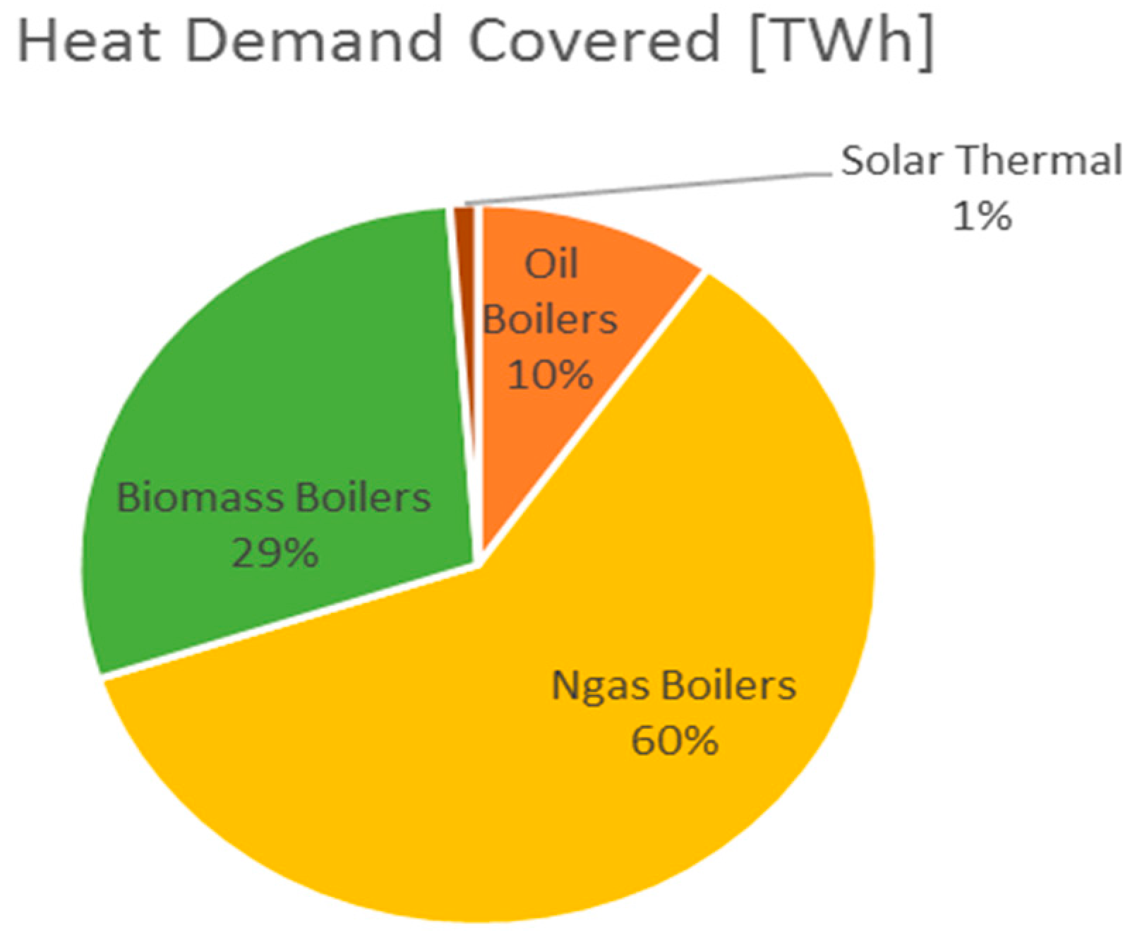
The heat demand has been covered mainly by natural gas boilers and biomass boilers. As shown in Figure 1, oil boilers are underused, like solar thermal technologies. In 2015, only 10% of the natural gas demand was covered by national production, the remaining 90% was covered by imports.

Table 2. Energy consumption by sources in the transport sector—Italy, 2014.

Consumption by Source	(Mtoe)	(TWh)
Jet fuels	3.722	43.287
Diesel	22.773	264.853
Gasoline	8.495	98.792
Gas	1.072	12.469
LPG	1.718	19.985
Electricity	0.900	10.464
Biofuel	1.065	12.391

shows the TFC by source in the transport sector. Here, the demand was 12.5% lower in 2014 than in 2004. The demand is still covered mostly by fossil fuels, mainly petroleum products (diesel and gasoline), then GPL and natural gas. The share of electricity is very low, and is mainly due to means of transport like trains and trams, whereas hybrid and electric cars are still uncommon; the contribution of biofuels is equal to 2.7% [29].

In the last 10 years, the energy demand in industry and transport decreased: in particular, the first one contracted its consumption by 31.4%; however, the consumption in both sectors went up a little in 2014 with respect to 2013 [29].

The energy demand in the residential sector experienced strong growth until 2013, but decreased in 2014, showing a total cut of 6.0% in the last decade. As a result, the share of total demand due to the residential sectors, from 2004 to 2014, increased by 5% until 25.3%. The consumption in the commercial sector went up by 20% from 2004 to 2008, but has cut steadily since there, and in 2014 was 13% lower than in 2008 [29].

4. Energy Planning Modelling: Italian Reference Model Implementation for Year 2014

The main inputs for creating a model using EnergyPLAN are energy demands, capacities, and costs of power plants (thermoelectric, cogeneration, renewables) and other renewable technologies.

The software gives the user the possibility to choose between two different types of analysis: technical simulation, whose goal is to reduce as much as possible the fossil fuel consumption and market simulation, whose goal is to reduce as much as possible the operation costs of the system. The difference between demand and supply is met if the power producing units can complete the task. The type of analysis selected in this case study is the technical one with a technical simulation of heat production based on heat demand. The units chosen to supply the heat demand are selected in the following order: (i) solar thermal; (ii) industrial CHP; (iii) heat production from waste; (iv) CHP heat; (v) heat pumps; (vi) peak load boilers. This also affects electricity production: under this regulation, the amount of heat that CHP units produce, and hence the amount of the produced electricity, is dependent on the heat demand at that time.

The user must provide, for a given year, the following data, on an hourly basis

• electricity demand;
• electricity import–export;
• renewable energy production: geothermal, photovoltaic, wind, river hydro, hydro with pump, and storage systems;
• residential cooling (air conditioning) and heating energy demand;
• transport energy demand;
• industrial energy demand.

After introducing input data, the model makes several calculations: it is possible to find the heat and electricity demands easily by dividing the annual demands keeping in mind of the internal hourly distributions.

4.1. Electricity

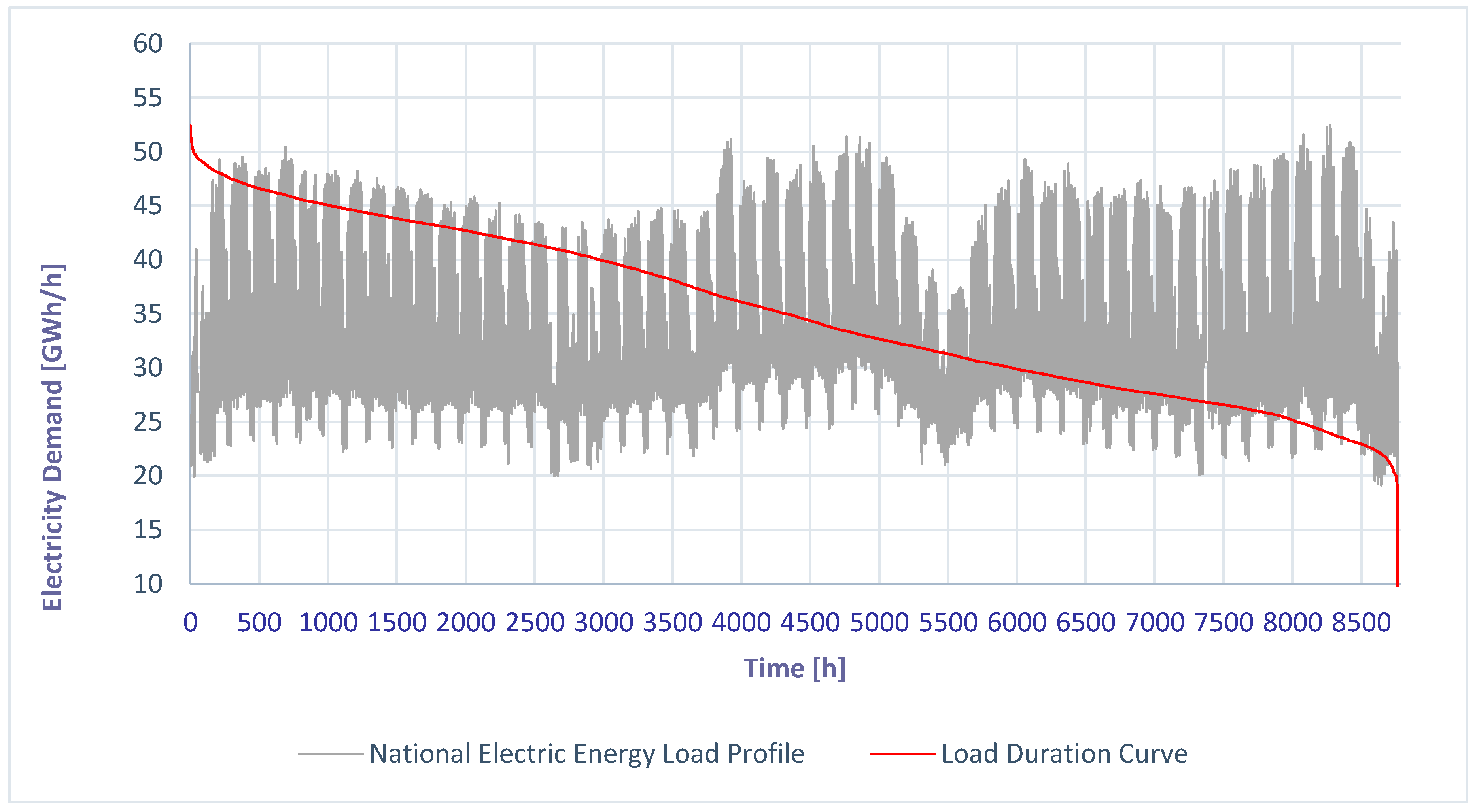
Electric energy demand data were provided, in this case, by TERNA (National Electricity Transmission Network), and are shown in Figure 2; these data are measured, so they do not need to be validated.

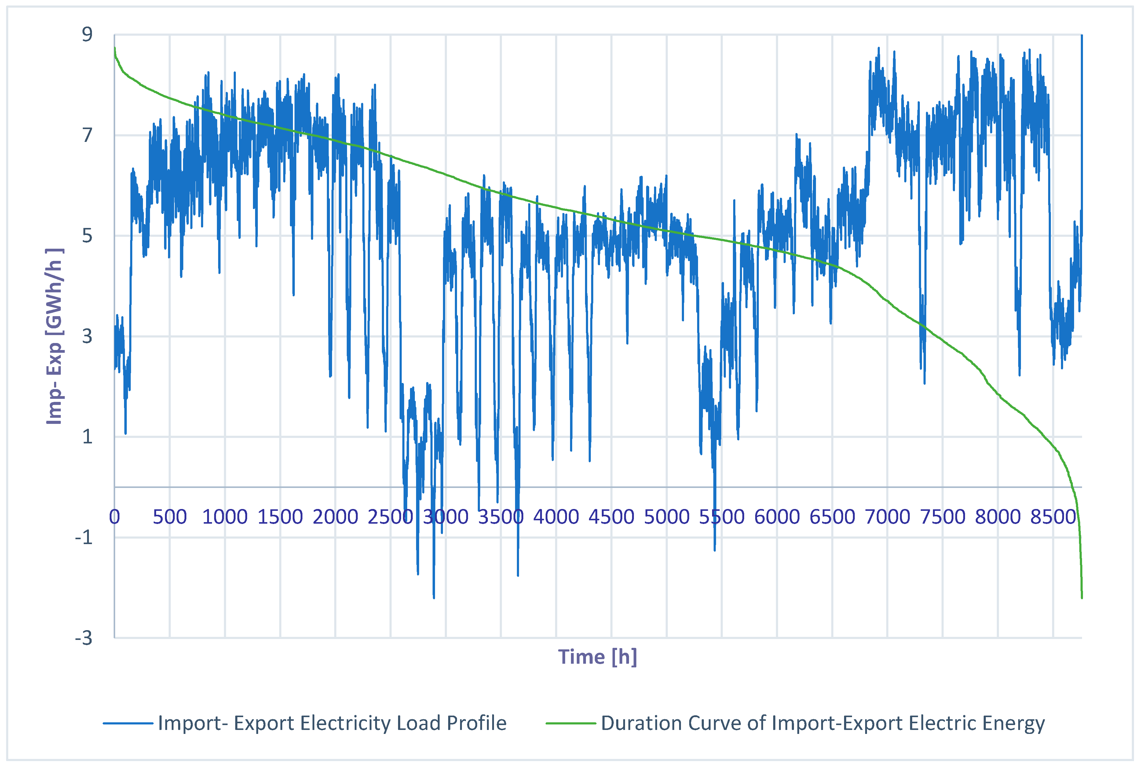
Regarding electric energy import and export, in the framework of the UCTE (Union for the Co-ordination of Transmission of Electricity), the Italian transmission grid is interconnected to external grids through 22 interconnection lines: 12 with Switzerland, 4 with France, 2 with Slovenia, 1 with Austria, 2 DC connections, 1 cable with Greece; furthermore, 1 cable connects the major Italian island of Sardinia to the mainland through the French island of Corsica; 1 additional AC cable links Sardinia and Corsica. In Italy, electricity imports cover almost 14% of the total electricity supply. In the EnergyPLAN model, the exchanges with external electricity markets, not included in the original model, are shown by the fixed import/export demand [25]. The input that must be entered in the model is the annual electricity demand (net of exports) for fixed exchange together with its hourly distribution, shown in Figure 3.

Data about imported and exported electricity are available on online database of the companies operating the different transmission grids involved (Italy, Austria, France, Switzerland, Slovenia, and France).

4.2. Heating

If individual heating is considered, it is possible to calculate the thermal energy demand for space heating and hot water based on the values of final consumption and efficiency production. “Fuel inputs” is used to define inputs to individual houses.

Table 3. Heating consumptions by sources in residential sector.

Total Consumption for Heating by Source	(Mtoe)	(TWh)	Efficiency (Estimate)	Heat Demand (TWh)
Biomass	5.720	66.52	0.85	56.55
Coal	0.00	0.00	0.80	0.00
Oil	1.800	21.00	0.85	17.84
Gas	10.490	122.06	0.90	109.85
Electric	0.530	6.16	-	-

shows heating consumptions by sources for the residential sector, provided by Odyssee Mure [31].

Furthermore, the heat demand from heat pumps is estimated to be equal to 30 TWh and the COP (Coefficient of Performance) is set equal to 3. The efficiencies of boilers are set at 0.85 for oil boiler, 0.9 for natural gas boiler and 0.8 for biomass boiler, respectively. There are not coal boilers.

The inputs required for individual solar thermal in EnergyPLAN model are the: hourly profile of the solar thermal production over the year, total annual solar thermal production, solar thermal share.

The total solar production in Italy for 2014 is provided by “Gestore Servizi Energetici” (GSE) [32] and it is equal to 2.09 TWh. This amount is subtracted from fossil fuels consumption output.

The houses, in percentage, equipped with solar panels are shown by the solar share: to calculate this data, the total surface of solar thermal panels installed must be estimated. In 2014, in Italy there were 3,535,000 m² of solar thermal panels installed. A typical solar installation uses is about 6 m², therefore it was assumed that there are approximately 589,167 solar installations in Italy. From the 2011 census in Italy there are 24,135,177 homes. From these data, we have a consideration of a solar thermal installation accounting for 2.4% of Italian houses.

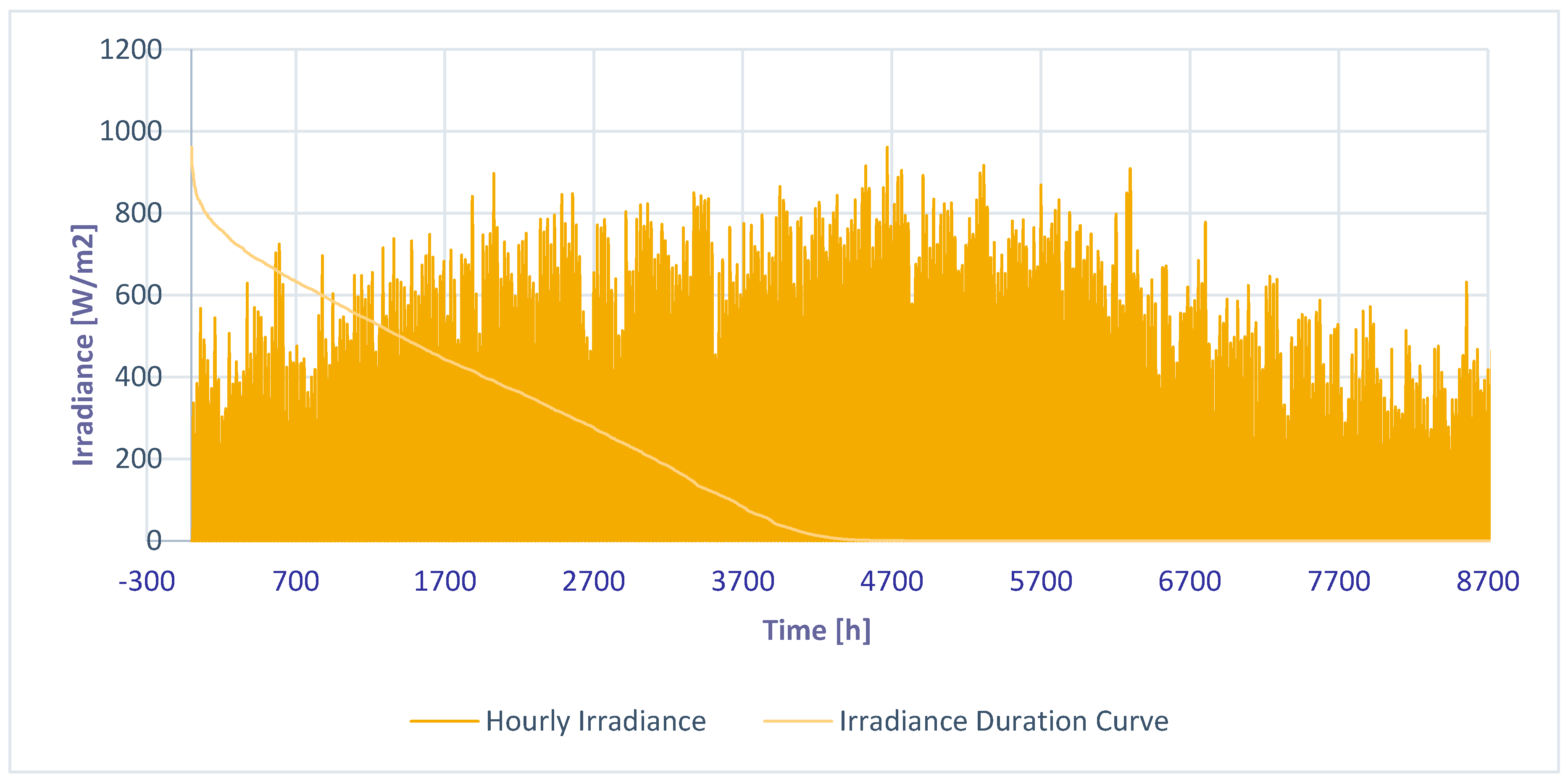
The model of a function shows the hourly solar insolation on a flat and tilted surface considering the hourly distribution for solar thermal. These data have been obtained from Meteonorm database [33] and collected for five representative Italian cities.

The distribution is then created for every location individually as an average of the insolation on the tilted and flat planes. The aggregated distribution curve in Figure 4 is calculated as an average of the five individual cities.

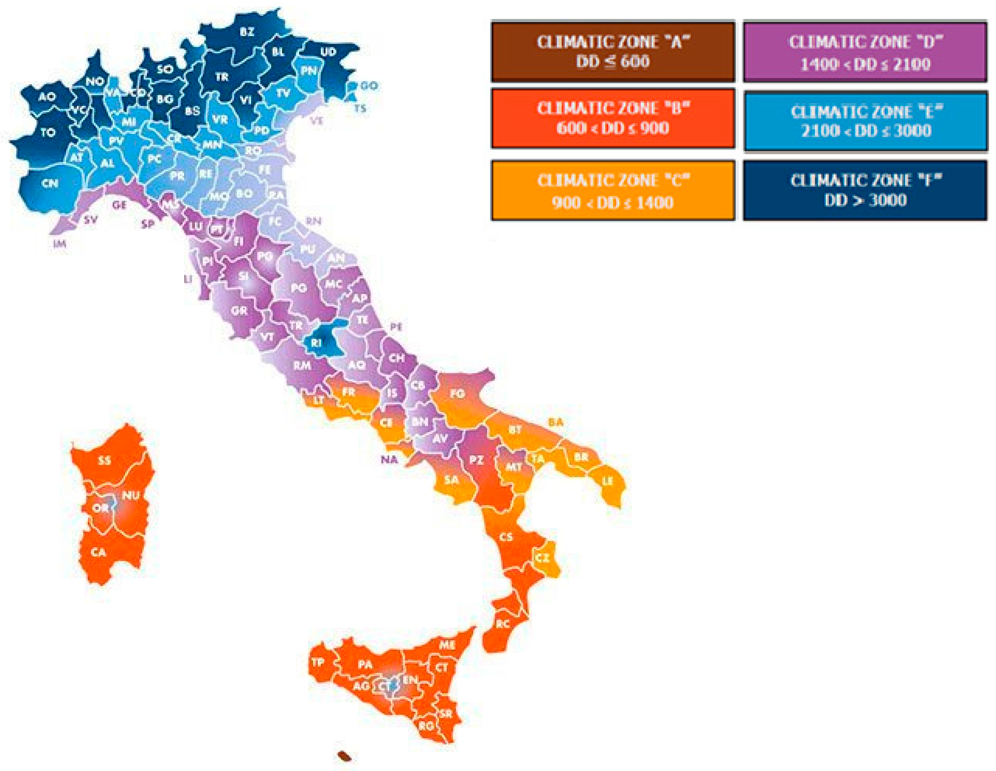
The hourly heat demand data are evaluated using the heat degree days method (HDD) at different locations (Palermo, Napoli, Torino, Milano, Roma) [25], each one representative of a typical Italian climatic zone. The Italian territory is, in fact, divided into six climatic zones (A, B, C, D, E, F), each one characterized by a range of degree days, as shown in the following Figure 5.

The classification of the national territory in six climatic zones has the purpose of limiting the energy consumption necessary for the operation of the heating systems, according to the Presidential Decree No. 412/1993. Each zone has a limitation concerning both the hours of operation of the heating systems per day and the months in which it is possible to use those systems, as resumed in

Table 4. Operating season and number of daily hours of operation per climatic zone.

ZONE A	ZONE B	ZONE C	ZONE D	ZONE E	ZONE F
6 h per day	8 h per day	10 h per day	12 h per day	14 h per day	No limitation
1 December–15 March	1 December–31 March	15 November–31 March	1 November–15 April	15 October–15 April	No limitation

.

Using the difference between the set-point and the outside temperature, with the difference reflecting the amount of heat that is required at that time, it can be calculated the HDD. The hourly distribution is obtained using the same methodology for each hour of the year by comparing the temperature measured outside with the set-point. If the outside temperature is above the set-point, then the HDD for that hour is assumed to be zero. The temperature within a building is usually 2–3 °C more than the temperature outside. Therefore, once the outside temperature drops below 15 °C outside, the inside temperature drops below 17–18 °C and the space heating within a building is usually turned on. During the day, the outside temperature used to estimate the space heating demand is referred to as the set-point and it is equal to 20 °C. During the night, space heating is activated only if outside temperature is below 0 °C, with a set point temperature of 15 °C.

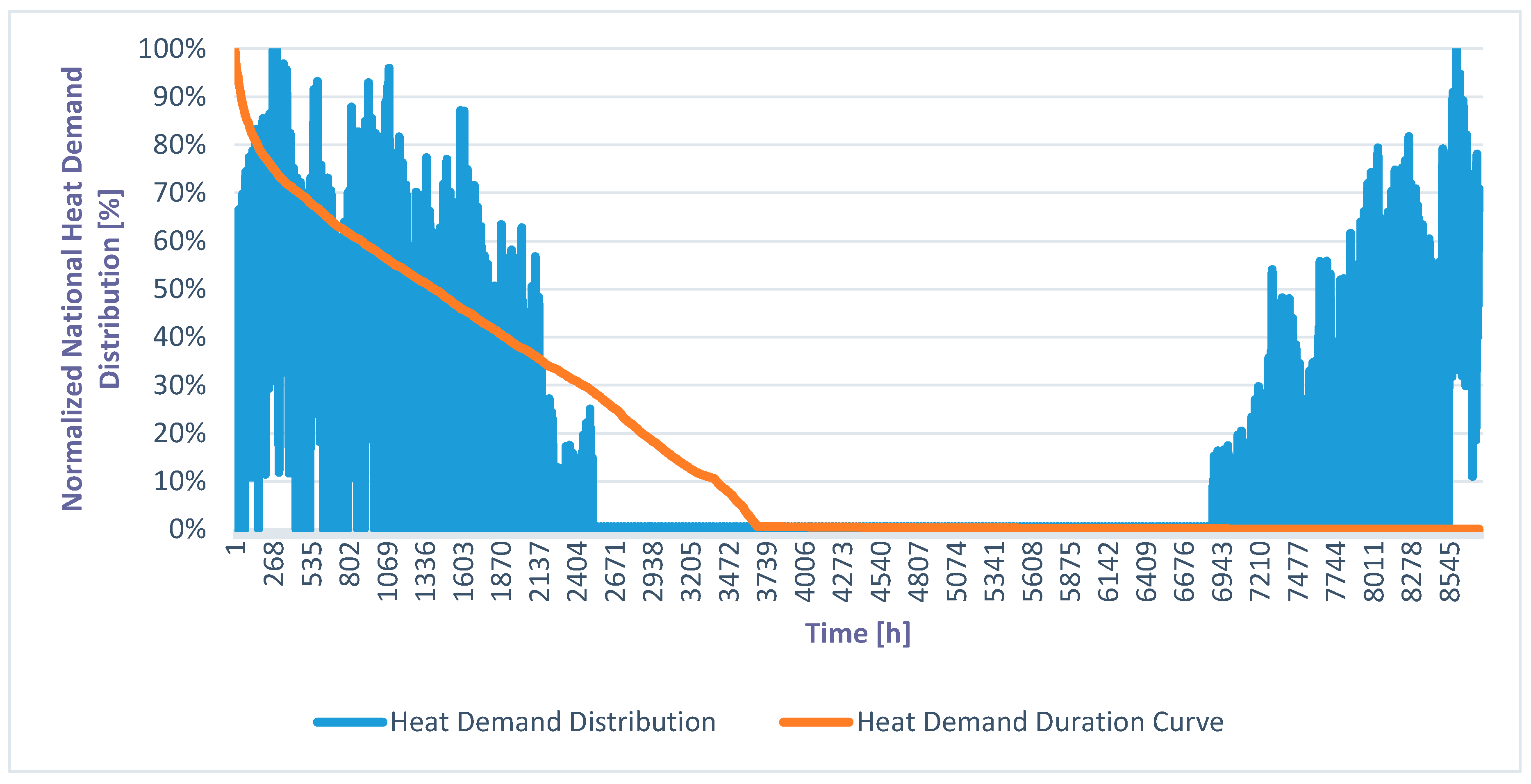
The aggregated distribution curve in Figure 6 is calculated as a weighted average of the five individual ones, considering the population of each zone.

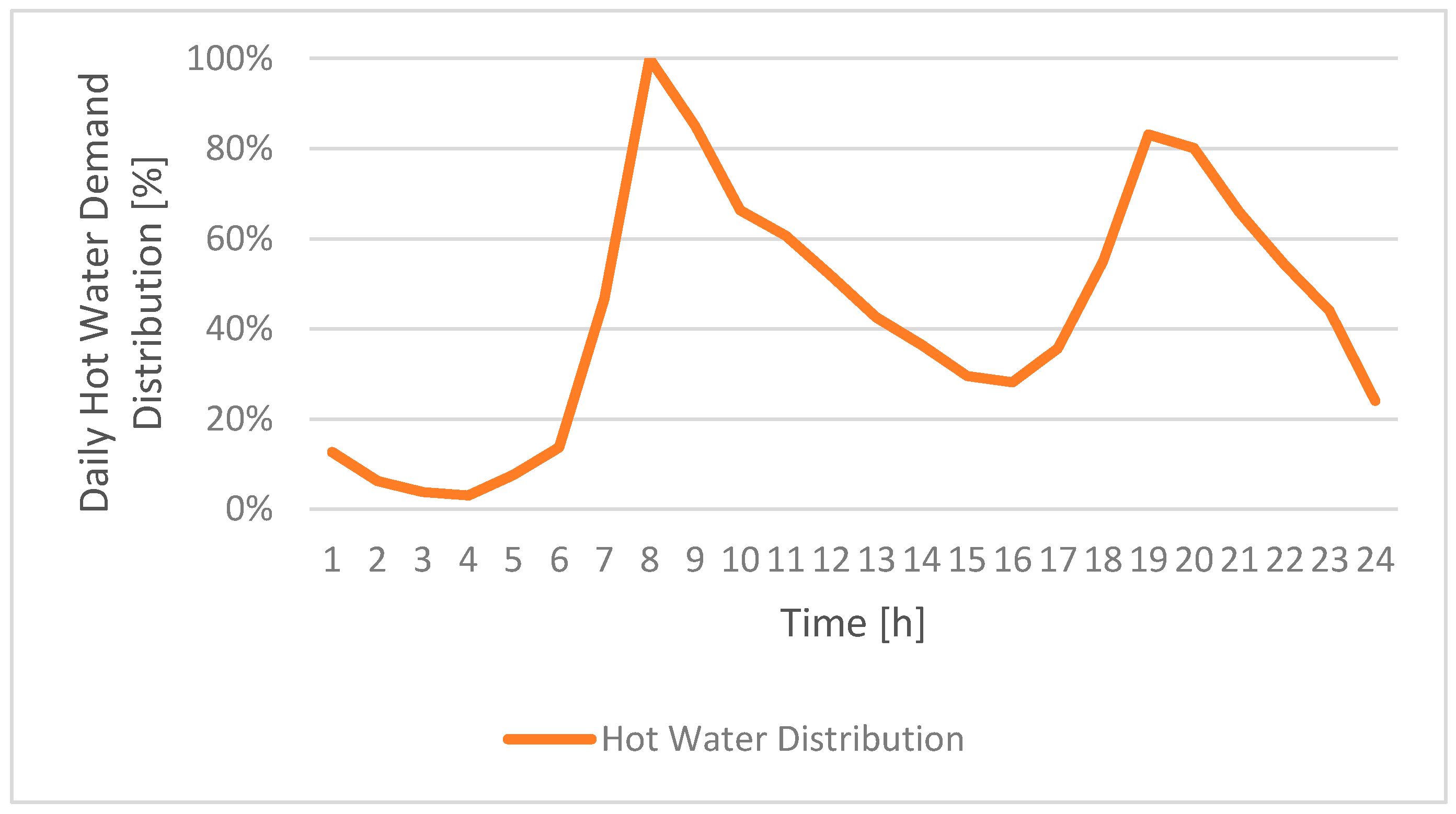
Cooking, showering, cleaning, and bathing in buildings requires the use of hot water. Differently from space heating, hot water demands do not significantly vary over the year, hence it is assumed to have a daily trend which is the same over the year [34]. The daily hot water demand value is calculated by identifying the requirement of hot water, in percentage, of the total annual heat demand and distributing the percentage over each day of the year. These data are currently available from the ENTRANZE [35] database (9% is assumed for Italy). The daily load profile is shown in Figure 7.

4.3. Cooling

Energy demand for cooling is usually assumed as function of weather conditions, but the experience proves that the cooling demand for non-residential buildings mostly depends on internal loads, independent from the climate, such as those generated by people and electrical appliances. However, in case of dwellings, several studies showed that internal loads play a marginal role for the overall cooling demand [36].

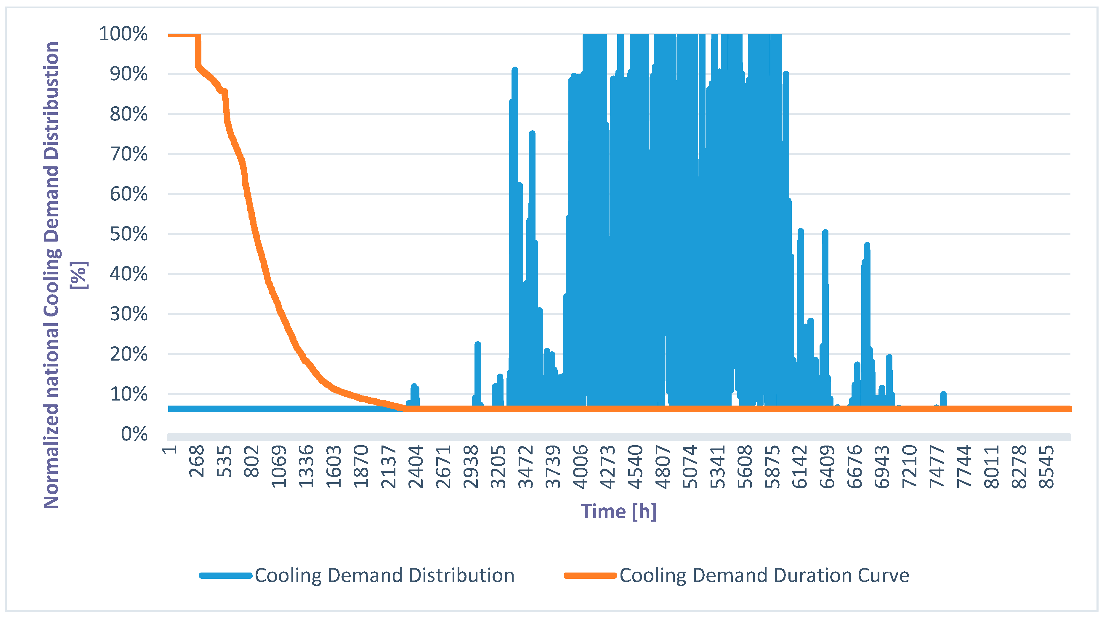
Thus, according this assumption, the load profile of the cooling demand was created using a similar methodology as the heating one. The cooling degree days (CDD) are estimated with an approach similar to HDD, but the set-point is usually different (26 °C in this case) and the cooling demand takes place every time the outside temperature is above the set-point. If the outside temperature is >29 °C the inside temperature is equal to the outside one −7 °C. Cooling is provided by air-conditioning (heat pumps) and measured in terms of how much electricity is consumed by these air-conditioning units. The load profile is shown in Figure 8.

Regarding district heating and cooling, EnergyPLAN gives the user the possibility to divide district heating into three main groups, based on the capacity of the plants. In this work, the three groups have been chosen after checking the data available on the website of AIRU (Italian district heating association) [37]. The hourly profile of the district heating demand must consider network losses. These are added as an additional baseload demand in the same way as hot water. Typically, these network losses range around 15%.

4.4. Industrial, Agriculture, Tertiary, and Transport Sectors

The final consumptions, divided by source, for the industrial, agriculture and tertiary sectors are shown in

Table 5. Final consumption by source in the industrial, agriculture, and tertiary sectors.

Consumption by Source and Sector		(TWh/Year)
Industry	Coal	26.36
	Oil products	25.99
	Gas	153
	Biomass	6.97
Various = Agriculture + Tertiary	Coal	0.00
	Oil products	29.78
	Gas	203
	Biomass	2.93

and were obtained by Odyssee Mure and MISE (Ministero dello Sviluppo Economico, Ministry of Economic Development) [31].

4.5. Transport

Regarding the transport section, the total final consumption for each type of fuel is available on the website Odyssee Mure.

4.6. Production and Generation

Electric and thermal capacities of thermoelectric and cogeneration plants are provided by TERNA [30].

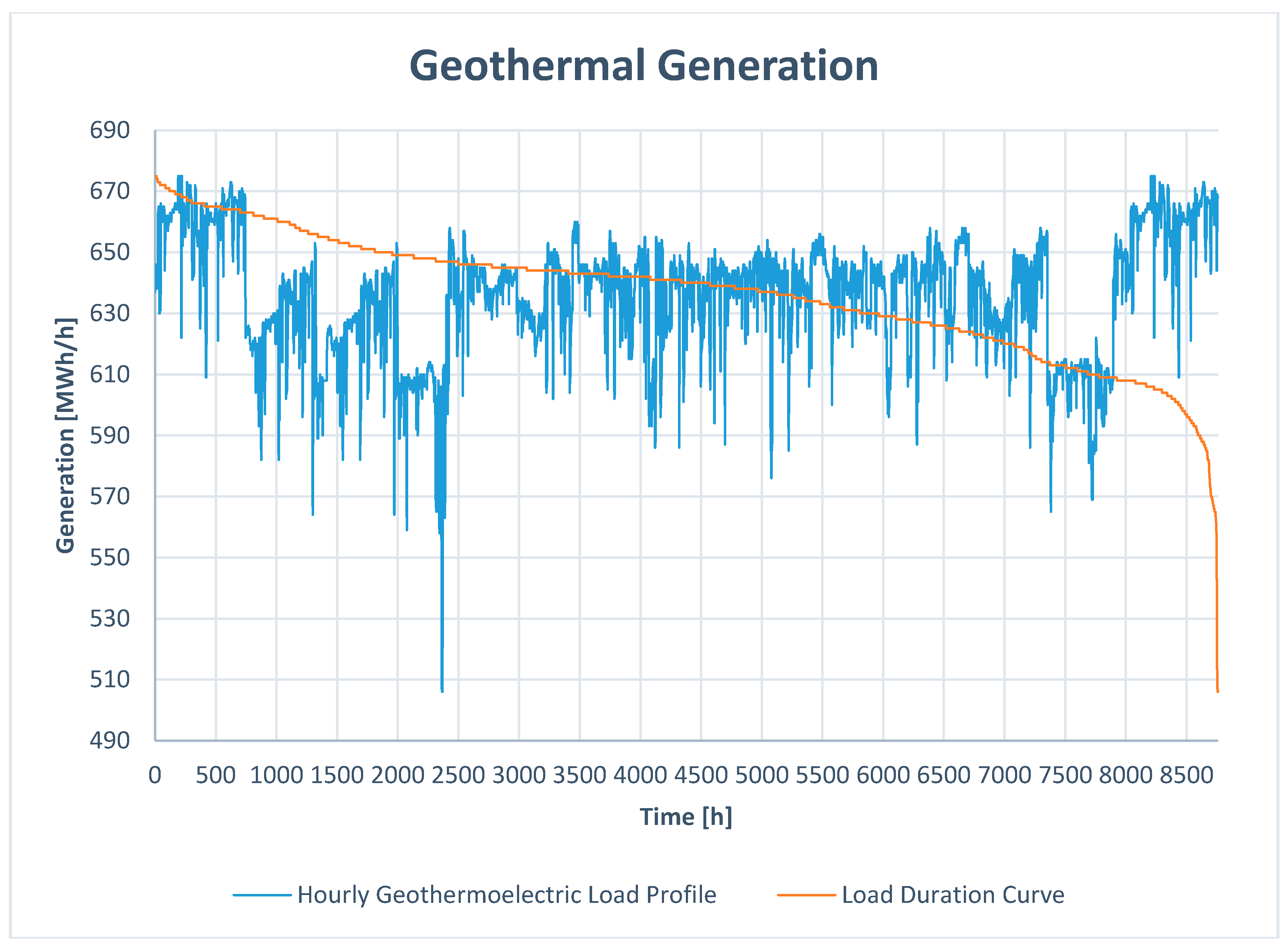
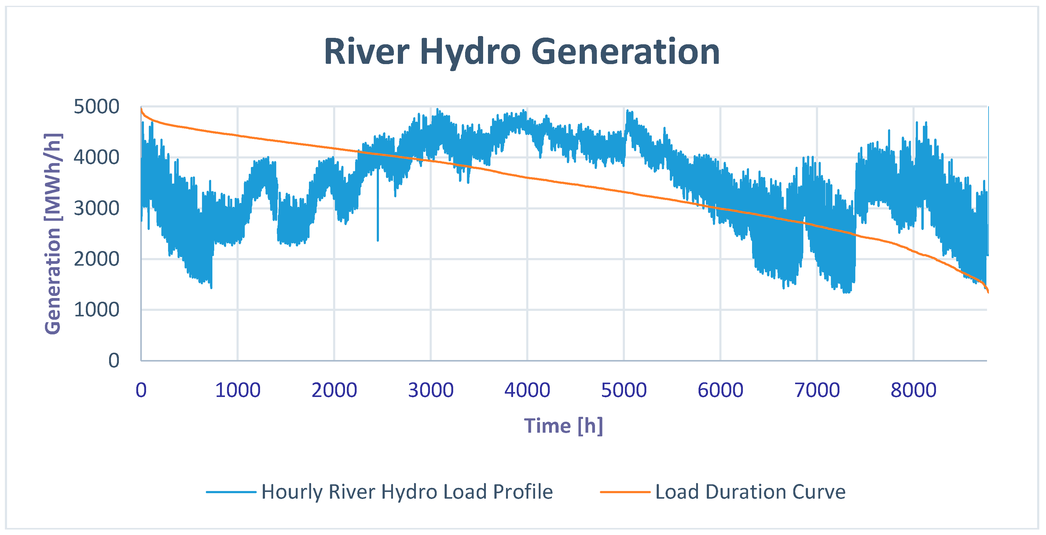
As for renewable energy source production data, previous works used production curves. In this case study, it was possible to obtain the hourly production measured values and the installed capacity of the plants, regarding the year 2014 from TERNA database. The input values in the software are shown in the following

Table 6. Electricity productions and installed capacities from RES for year 2014 in Italy.

Renewable Energy Sources	Installed Capacity (MW)	Production (TWh/Year)
Geotermoelectric	821	5.92
Dammed hydro	9582	28.54
Run of river plants	5059	30
Wind	8700	15.18
Photovoltaic	18,609	22.3

.

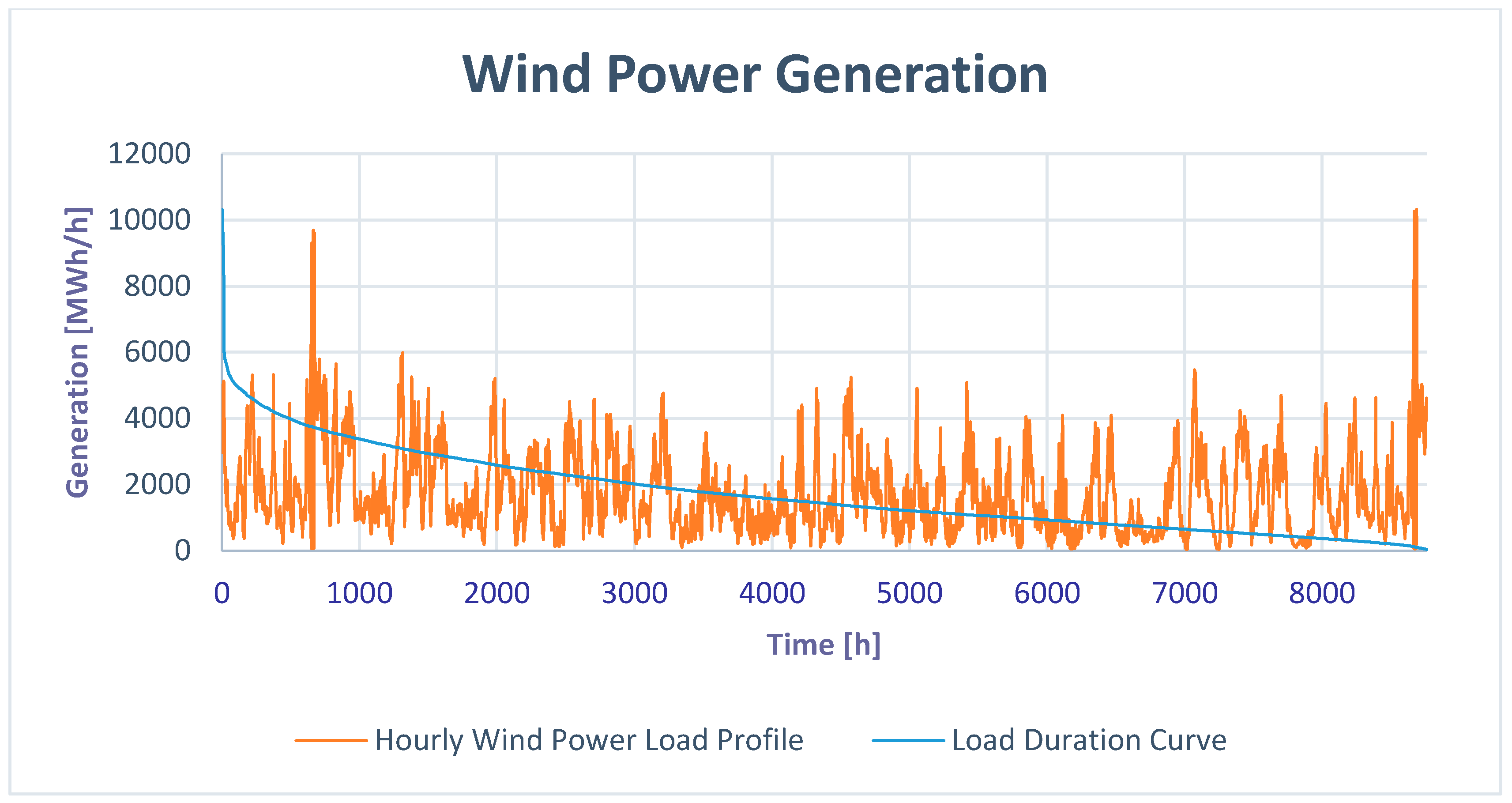
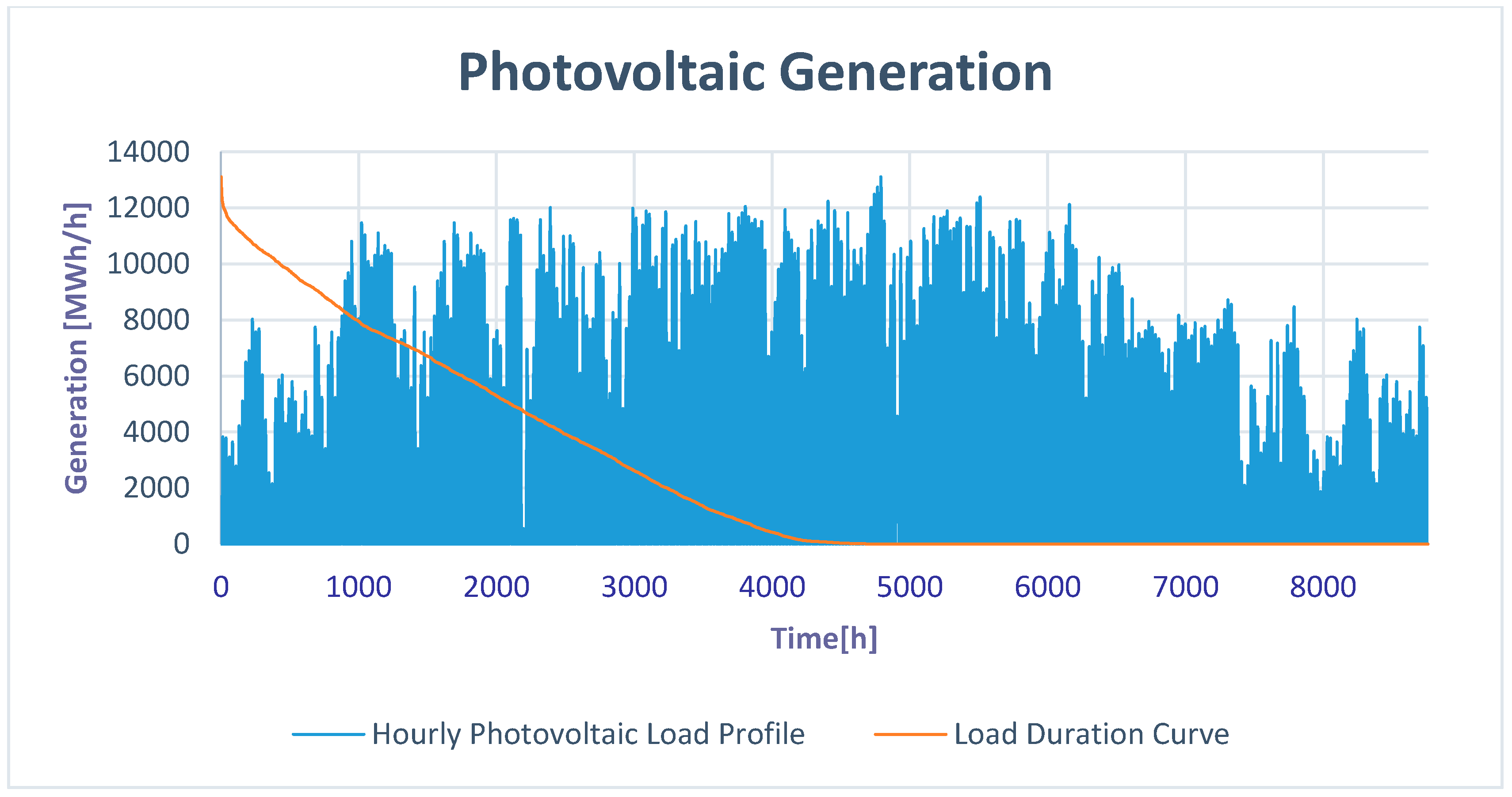
The data regarding the production of electric energy from renewables are entirely based on measured data, so there is no need for validation. The time profiles of RES productions in 2014 are shown in Figure A1, Figure A2, Figure A3 and Figure A4 in Appendix A.

The electricity production input from intermittent renewable energy sources such as wind power is found by multiplying the capacity by the specified hourly distribution. However, different future technologies will lead to either lower or higher productions. Therefore, it is possible to specify a correction factor to change the distribution and increase the annual production. The factor changes the production in such a way that the production remains the same at hours with either no production or full production, while the other values are adjusted relatively [25].

The stabilization share is defined as the ratio of the installed capacity of renewable plant suitable to contribute to the grid stability, ranging between 0 and 1. The only intermittent renewable energy technologies that can do that are hydro power plants. Therefore, the stabilization share will be set to 0.

For various production units in the model (district heating plants, cogeneration plants, and traditional power plants), the distribution across fuel types is stated as input, divided into coal, oil, natural gas, and biomass. Such fuel consumption data are provided by TERNA and by AIRU.

The thermal and electricity production by waste source and electricity production by biofuels and biogas data are provided by AIRU. Only pumped hydroelectric energy storage (PHES) is in use in Italy. The total capacity for pumped-storage is 7669.1 MW.

4.7. Validation: Heating and Cooling Demand Distribution for the Residential Sector, CO₂ Emissions, and Final Fuel Consumption

To validate the data about heating and cooling demand profiles in the EnergyPLAN model, a TRNSYS simulation was developed.

This energy tool, through a dynamic simulation, can give, as a result, the thermal behavior of a building.

In order to simulate the behavior of the entire Italian building stock and hence the profile of the national cooling and heating demands, it was necessary to collect statistical data and find the most common building types and their distribution in the Italian building stock.

Each type of building considered for the simulations, belongs to the “National Building Typology Matrix” of TABULA [38], a project developed by “Politecnico di Torino”. TABULA Project aimed at assessing and improving the energy performance of the existing buildings. The national “building typology” has been classified according to the following criteria:

• building age;
• building size.

Eight age classes were identified:

• class I, up to 1900—the 19th Century;
• class II, from 1901 to 1920—the beginning of the 20th century;
• class III, from 1921 to 1945—the period between the two world wars;
• class IV, from 1946 to 1960—the post-war period and the reconstruction;
• class V, from 1961 to 1975—towards the oil crisis;
• class VI, from 1976 to 1990—first Italian regulations on energy efficiency;
• class VII, from 1991 to 2005—recent regulations on the energy performance of buildings in Italy (from Law No. 10/1991 to the Legislative Decree No.192/2005);
• class VIII, after 2005—more restrictive energy performance requirements (implementation decrees of Legislative Decree no. 192/2005 and regional laws).

For each age class, the following sub-classes were identified, based on the mean size of the building:

• single-family house: one or two floors single flat, detached o semi-detached house;
• terraced house: one or two floors single flat, terraced;
• multi-family house: small building characterized by a limited number of apartments (e.g., from two to five floors and up to 20 apartments); apartment block, big building characterized by a high number of apartments (e.g.,: more than four floors and more than 15 apartments).

The geometric modeling of type-buildings was performed with a Google SketchUp plug-in, “Trnsys3d”. The first step when building the thermal zones in Trnsys3D was to find the dimensions of each single thermal zone: such data were taken from the TABULA project and are shown in Table 6.

The model created was loaded on the TRNSYS “Simulation Studio” interface.

The thickness and the material used to characterize the building type (Type56) in this work were taken from the TABULA Project [38].

Once the characteristics of a given building were defined, it is possible to describe the cooling and heating systems using the types of the software “Simulation Studio”. The total heating demand was calculated based on an actual demand. The set point for heating demand is 20 °C, while for cooling demand is 26 °C. The infiltration represents the number of air volumes in the unit of time entering in the building from the outside through the windows due to their inadequate closure. Here, it was fixed at 0.6 vol/h. Gains define internal inputs. In this case, they are given by people (based on statistics of the ISTAT), internal equipment (like PC with monitors), lighting system. It was considered that computers and artificial lighting (equal to 5 W/m²) were turned on from 6 p.m. to 12 p.m.

The heating demand of each type of building is also strictly connected to the climatic zone considered.

A TRNSYS simulation has been run for each element of the “Building Typology Matrix”, for each Italian climatic zone, totaling 160 simulations. The results given by the tool is the hourly cooling and heating demand in a year of the single building-type in a specific area.

Type “Weather data” was used for the weather conditions in five different Italian cities, one for each climatic zone: Bolzano, Bologna, Roma, Napoli, and Messina.

Type “Heating season” has been used to define the months of the operation for the heating system, which is different for each zone considered, according to the Presidential Decree no. 412/1993. Two specific daily operating periods were considered, for winter and summer respectively, selected according with data provided by the National Institute for Statistics, ISTAT [39].

To evaluate the hourly cooling and heating demand over an entire year for each type of building, an analysis of the building stock of that area was required. Such data were obtained from ISTAT [40] (

Table A1. Main geometrical data of the building types belonging to the Italian middle climate.

Building Size Class	Building Age Class	Gross Heated Volume [m3]	Net Floor Area [m2]	Gross Floor Area [m2]	Compactness Factor [m−1]	Number of Floors	Number of Apartments
Single family houses	I	533	139	-	0.77	2	1
	II	448	115	-	0.82	2	1
	III	455	116	-	0.81	2	1
	IV	583	162	-	0.75	2	1
	V	679	156	-	0.73	2	1
	VI	725	199	-	0.72	2	1
	VII	605	172	-	0.73	2	1
	VIII	607	174	-	0.72	2	1
Terraced houses	I	500	123	-	0.51	2	1
	II	478	112	-	0.51	2	1
	III	428	113	-	0.49	2	1
	IV	400	111	-	0.51	2	1
	V	374	89	-	0.52	2	1
	VI	434	125	-	0.69	2	1
	VII	426	111	-	0.67	2	1
	VIII	519	127	-	0.64	2	1
Multy-family houses	I	2684	-	647	0.55	2	5
	II	4113	-	1306	0.54	2	16
	III	4388	-	1164	0.51	4	20
	IV	3076	-	961	0.51	3	12
	V	3074	-	934	0.54	5	10
	VI	4136	-	1209	0.48	3	12
	VII	3526	-	1120	0.54	3	15
	VIII	2959	829	-	0.5	3	13
Apartment blocks	I	3745	-	1058	0.35	5	16
	II	11029	-	2280	0.47	4	40
	III	7197	-	2249	0.46	5	30
	IV	5949	-	1763	0.46	4	24
	V	9438	-	2869	0.46	8	40
	VI	12685	-	4125	0.37	6	48
	VII	9912	-	3271	0.43	6	36
	VIII	8199	2124	-	0.4	7	31

,

Table A2. Percentage of buildings per number of apartments per age of construction, ISTAT 2001.

Age of Construction	Number of Apartment per Building
	1	2	3–4	5–8	9–15	More than 16
Before 1919	37%	20%	17%	12%	7%	7%
From 1919 to 1945	35%	18%	14%	10%	8%	14%
From 1946 to 1961	23%	16%	12%	12%	12%	25%
From 1962 to 1971	19%	16%	12%	10%	12%	30%
From 1972 to 1981	22%	17%	13%	12%	12%	24%
From 1982 to 1991	24%	15%	12%	13%	12%	24%
After 1991	22%	13%	12%	16%	15%	22%

,

Table A3. Contiguity per age of construction, ISTAT 2001.

Age of Construction	Contiguity
	None	1 or More
Before 1919	27%	73%
From 1919 to 1945	35%	65%
From 1946 to 1961	51%	49%
From 1962 to 1971	62%	38%
From 1972 to 1981	69%	31%
From 1982 to 1991	69%	31%
After 1991	72%	28%

,

Table A4. Percentage of buildings per age of construction, ISTAT 2001.

Age of Construction	Percentage
Before 1919	15%
From 1919 to 1945	11%
From 1946 to 1961	14%
From 1962 to 1971	17%
From 1972 to 1981	17%
From 1982 to 1991	12%
From 1991 to 2001	7%
After 2001	7%

and

Table A5. Number of buildings per climatic zone.

Climatic Zones	Number of Buildings	%
A	4875	0.04
B	699,573	5.74
C	2,710,544	22.24
D	2,858,016	23.45
E	5,191,960	42.60
F	722,730	5.93
Total	12,187,698	100

in Appendix A), again, as summarized in the following:

• percentage of buildings per number of apartments per age of construction;
• contiguity per age of construction;
• percentage of buildings per age of construction.

The tables were used to identify the building size classification, according to the TABULA Project.

The result brought to the

Table 7. Building size classification per age of construction.

Age of Construction	Single Family House	Terraced House	Multi-Family House	Apartment Block
Before 1919	10%	27%	56%	7%
From 1919 to 1945	12%	23%	51%	14%
From 1946 to 1961	12%	11%	52%	25%
From 1962 to 1971	12%	7%	51%	30%
From 1972 to 1981	15%	7%	54%	24%
From 1982 to 1991	17%	7%	52%	24%
From 1991 to 2000	16%	6%	56%	22%
After 2001	16%	6%	56%	22%

, in which another age of construction class was introduced, assuming that the size distribution was the same of the previous age class.

Considering the overall percentage of residential building stock classified per age of construction, it was possible to obtain the matrix of the distribution incidence of the building types according to the TABULA classification (

Table 8. Matrix of the distribution incidence of the building-types according to the TABULA classification.

Age of Construction		Single Family House	Terraced House	Multi-Family House	Apartment Block
I	Before 1919	1%	2%	4%	1%
II	From 1900 to 1919	1%	2%	4%	1%
III	From 1919 to 1945	1%	2%	6%	2%
IV	From 1946 to 1960	2%	2%	7%	4%
V	From 1962 to 1971	2%	1%	8%	5%
VI	From 1972 to 1991	5%	2%	16%	7%
VII	From 1991 to 2000	1%	0%	4%	2%
VIII	After 2001	1%	0%	4%	1%

).

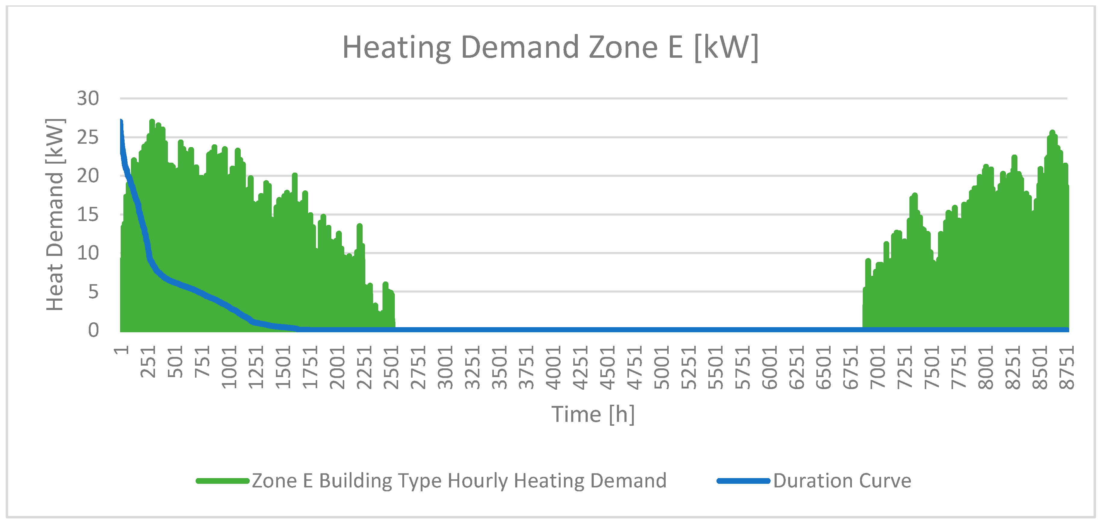
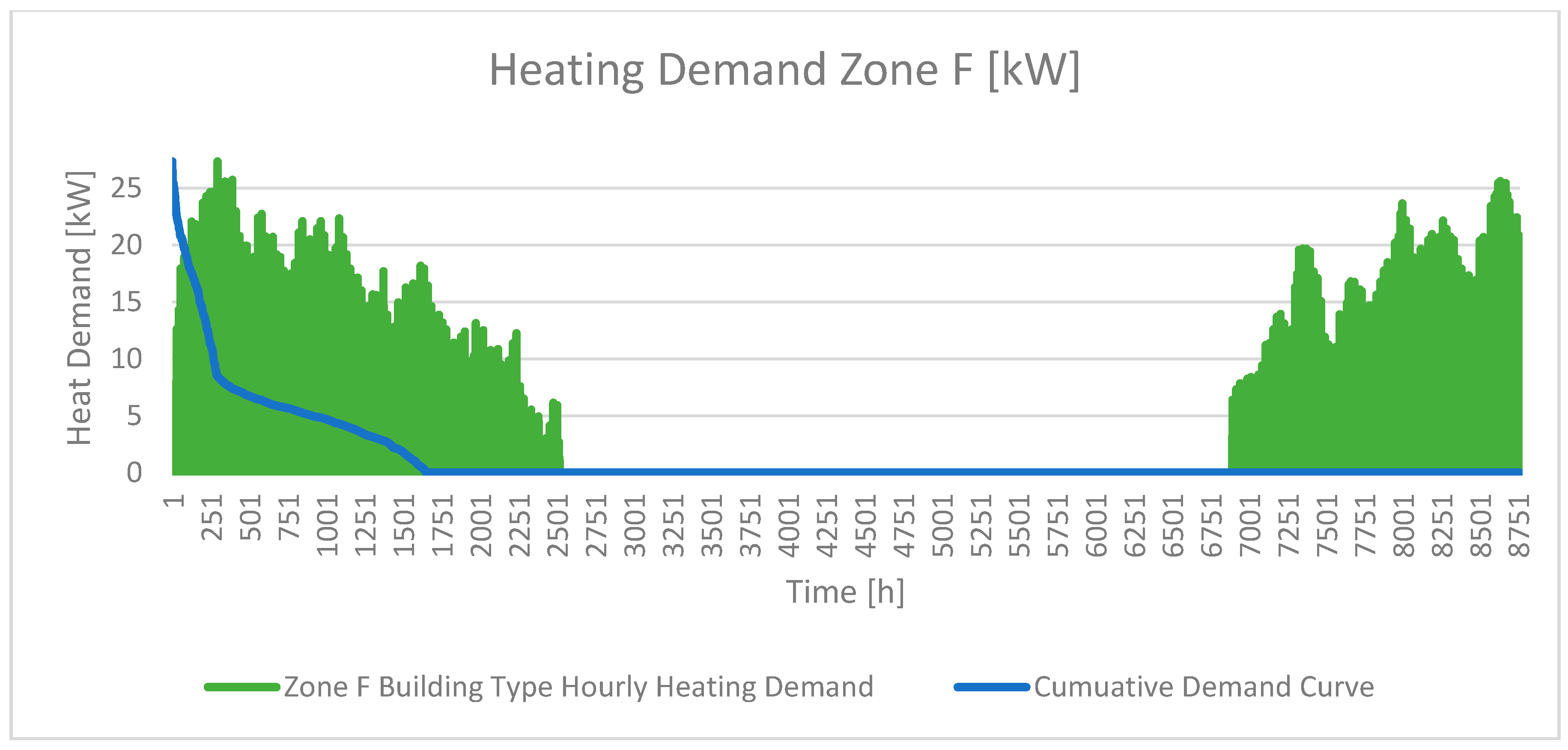
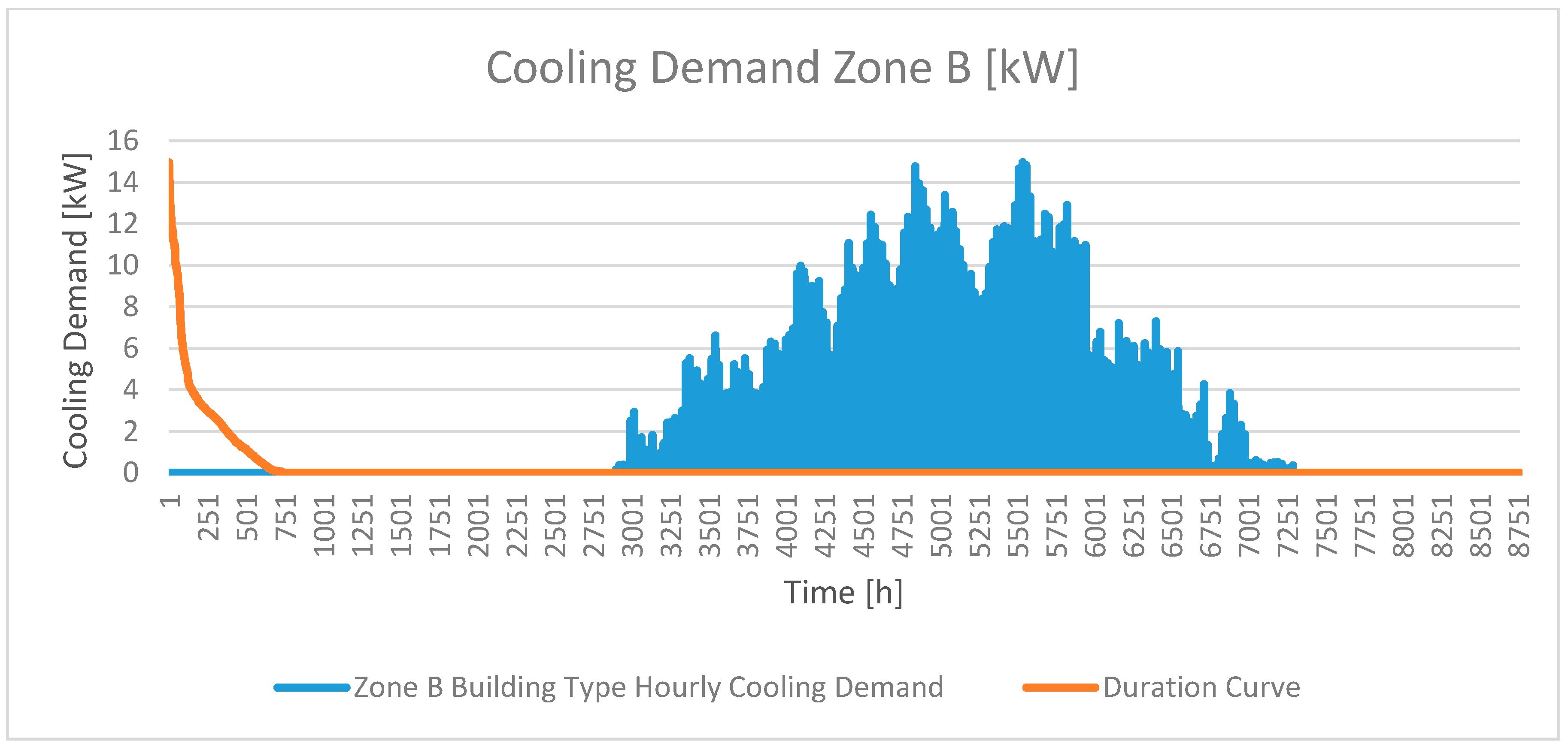
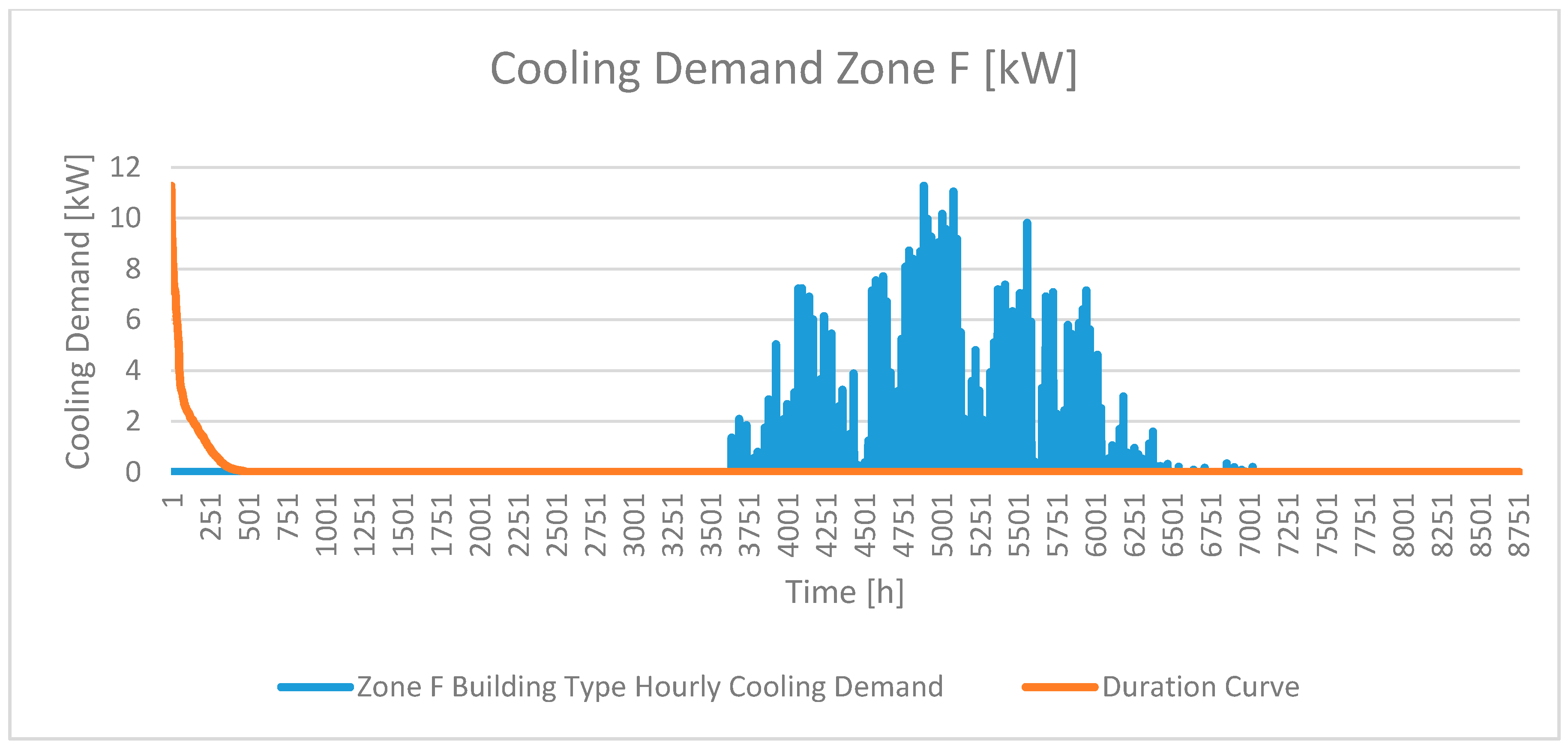
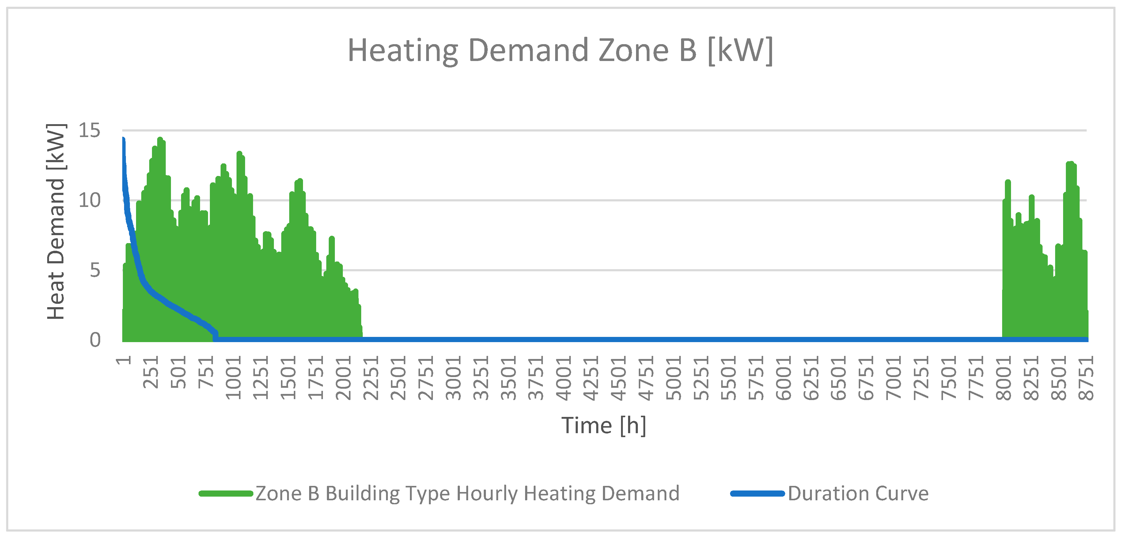
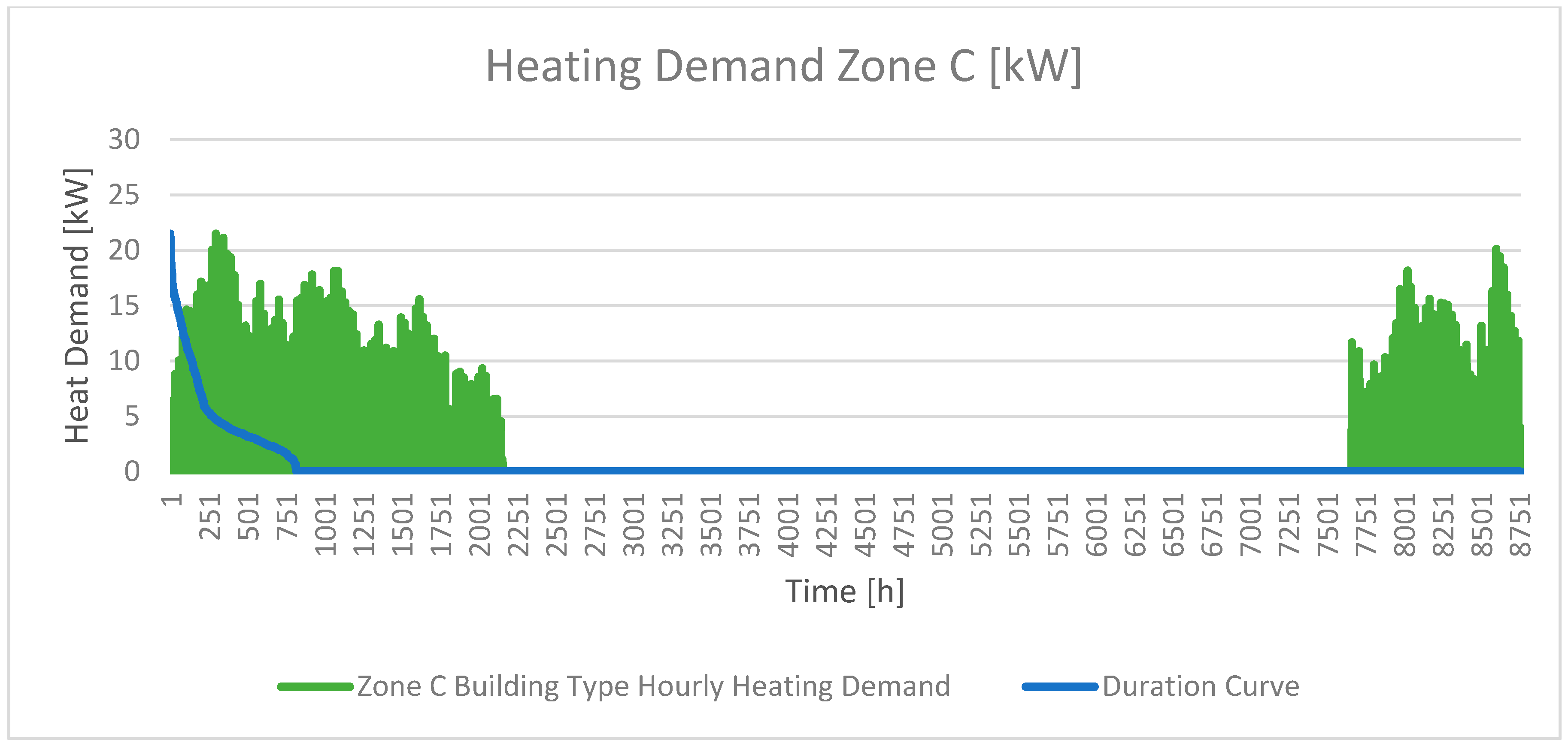
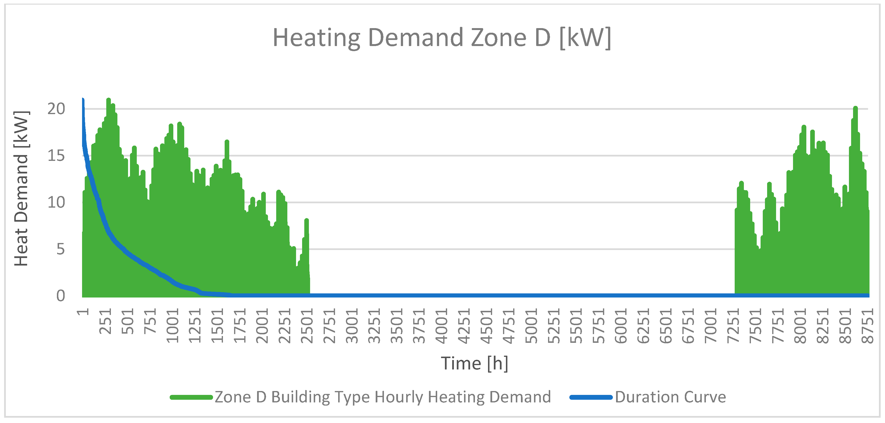
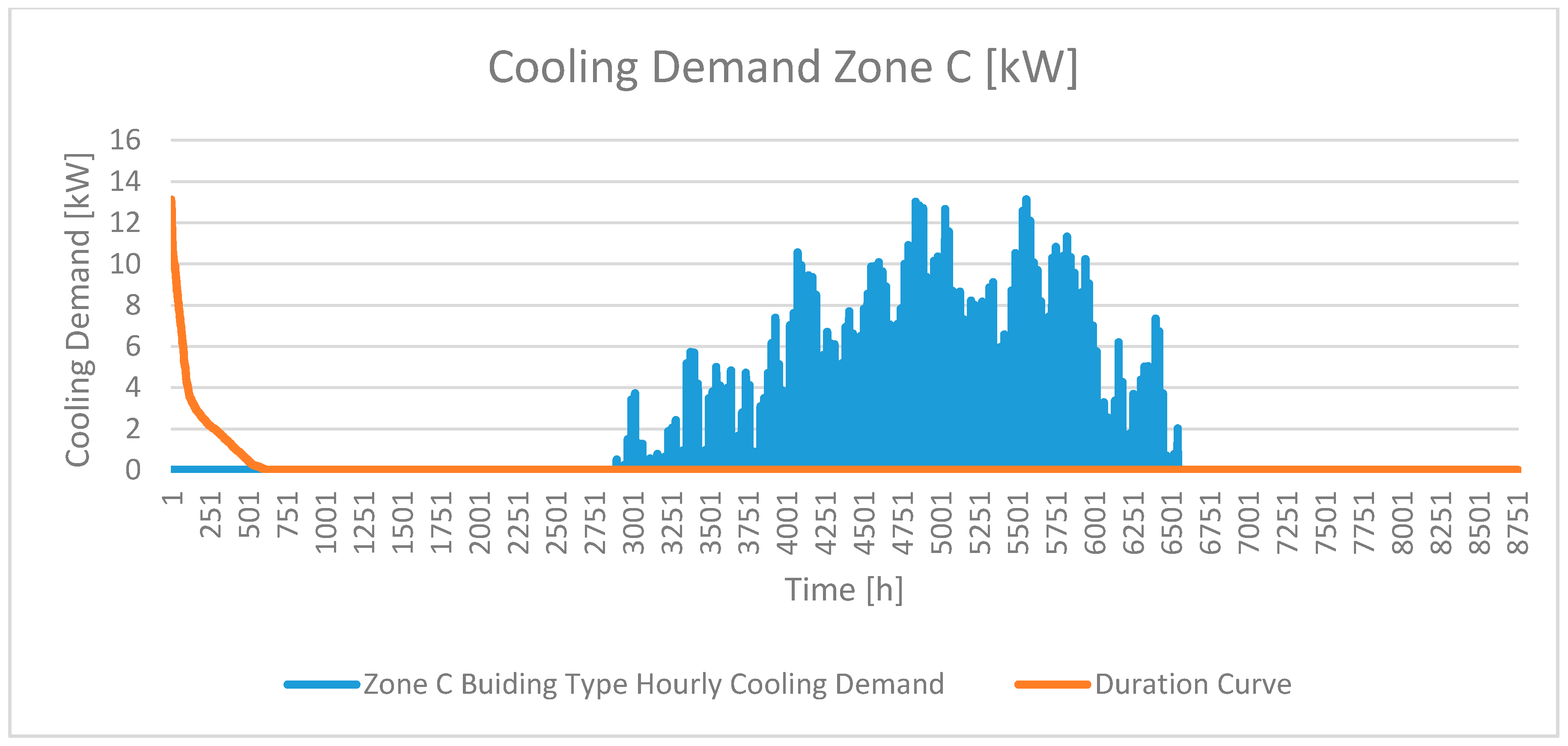
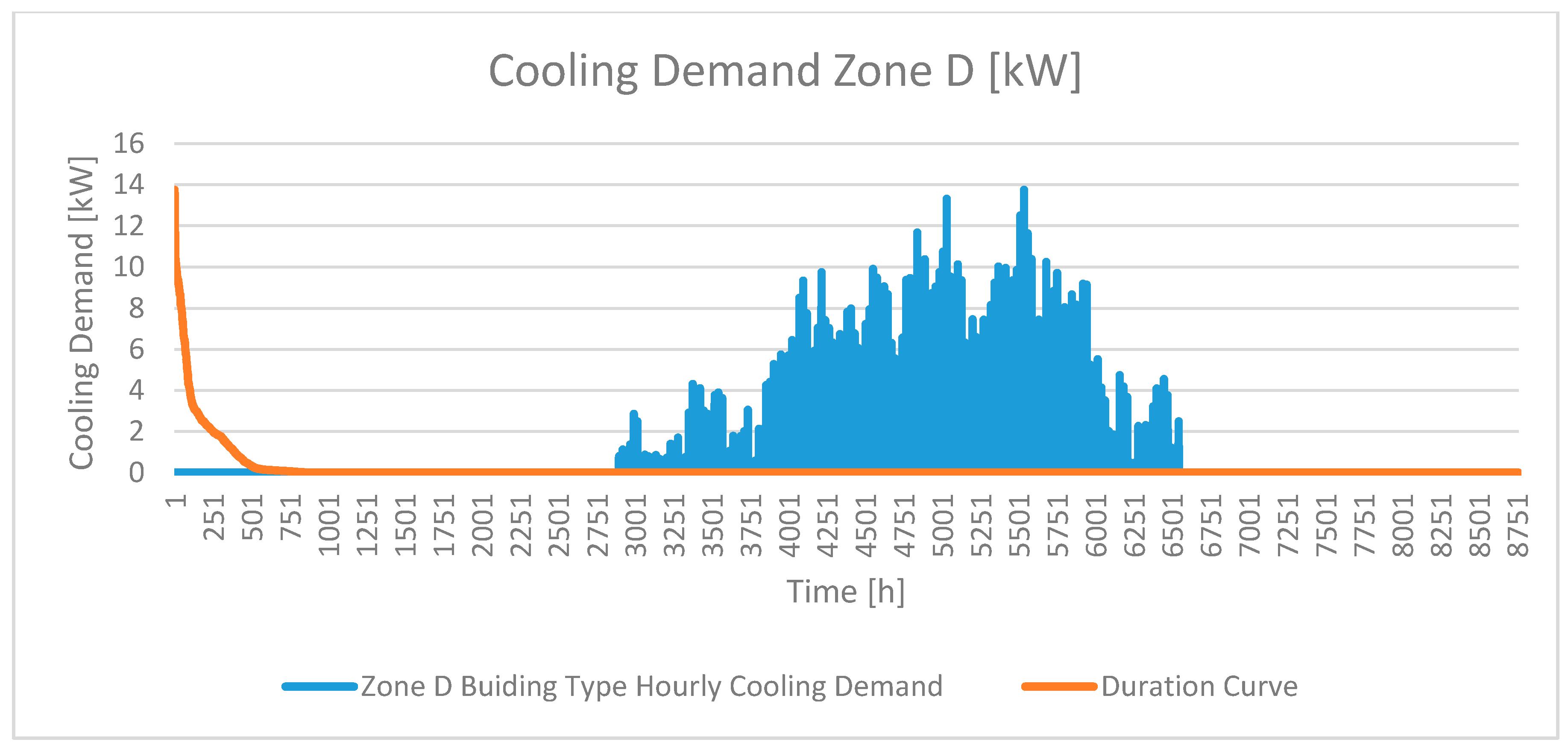
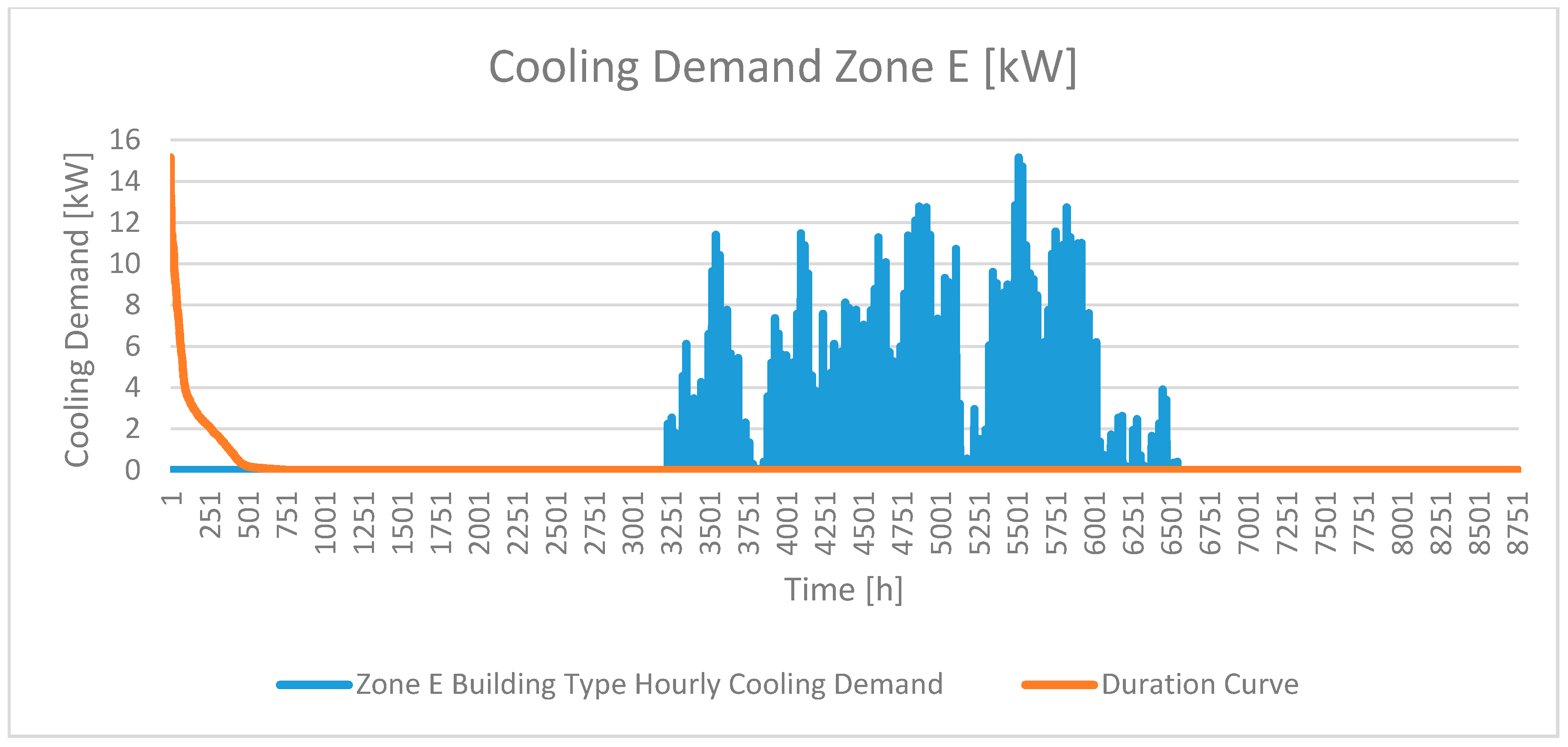
For each climatic zone, a simulation was run for each element of the “Building Typology Matrix". The result was multiplied by its frequency of distribution in the Italian building stock. This way, it was possible to obtain an hourly demand profile for each building-type and for each climatic area (Figure A5, Figure A6, Figure A7, Figure A8, Figure A9, Figure A10, Figure A11, Figure A12, Figure A13 and Figure A14 in Appendix A).

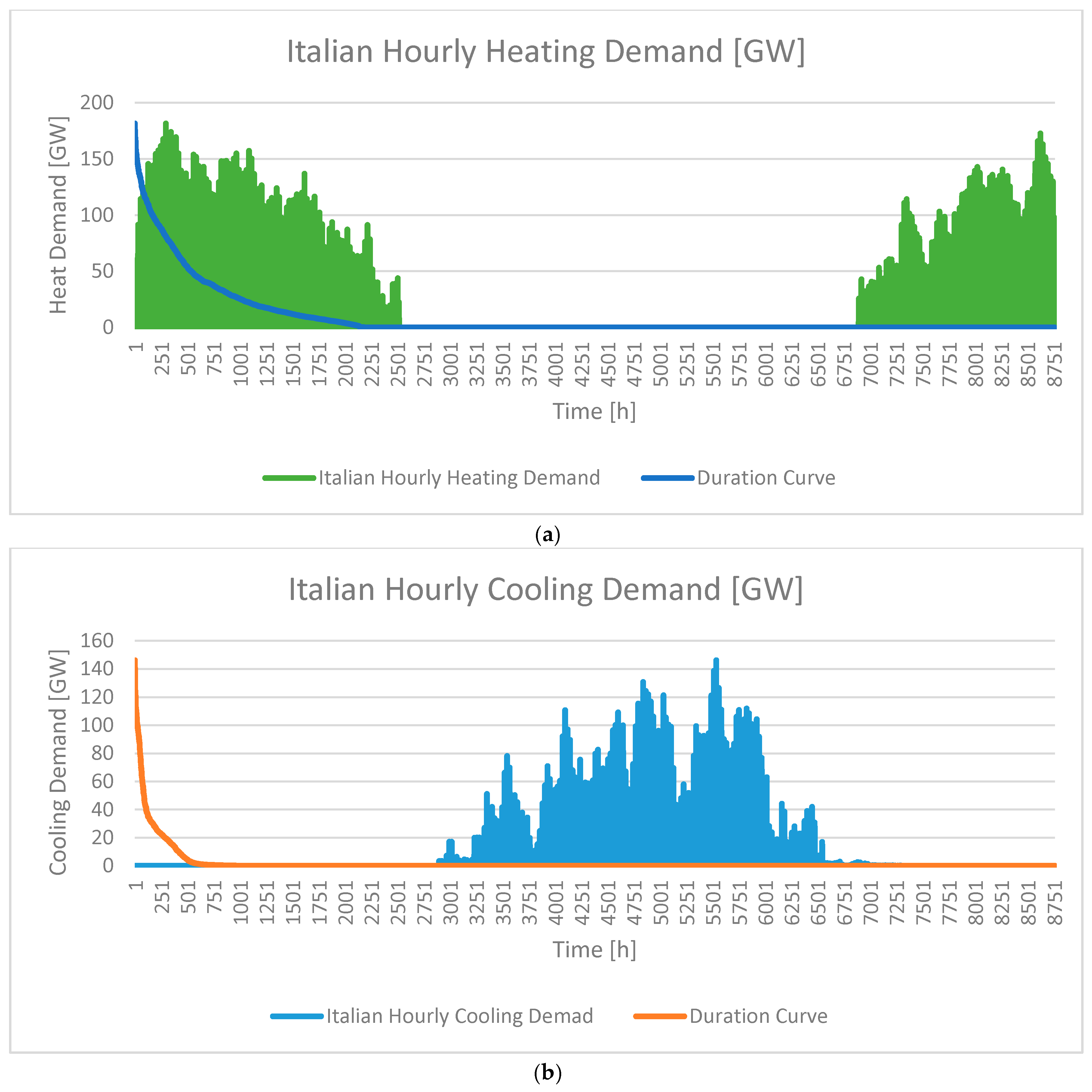
The aggregated hourly demands for heating and cooling were obtained as a weighted average of those calculated for each climatic zone (according to the number of buildings per climatic zone), multiplied by the number of buildings in Italy, the results are shown in Figure 9.

The national heating and cooling distributions obtained in such way were used respectively as input heating and cooling demand distributions in the EnergyPLAN model, giving the same output values.

Furthermore, the reference scenario created has been validated through a comparison between the CO₂ emissions estimated through the EnergyPLAN model (337.66 Mt) with that provided for the year 2014 by EDGAR, Emission Database for Global Atmospheric Research (337.61 Mt); the difference is negligible, confirming the reliability of the results provided by EnergyPLAN.

EnergyPLAN final fuel balance output data was also compared with that provided by the IEA (International Energy Agency): according to the IEA, Italian fuel consumption in 2014 was 1707 TWh, compared to the EnergyPLAN value of 1629 TWh; so, an acceptable difference (<5%) was found.

As a summary, the model created to simulate the reference scenario was successfully validate by comparison with the measured data available in literature. Such a reference scenario was the first step to develop future scenarios, suitable to evaluate possible strategies aimed at improving energy efficiency and reducing GHG emissions.

5. Analysis of Future Scenarios

The future scenario for the year 2050 was created on the basis of data taken from “Pathways to Deep Decarbonization in Italy” [4], a report presented by the Italian National Agency for New Technologies, Energy and Sustainable Economic Development (ENEA) and the Fondazione ENI Enrico Mattei (FEEM).

The ENEA report presents three alternatives to reach a deep decarbonization: carbon capture and storage (CCS), energy efficiency (EFF), demand reduction (DR).

The energy efficiency pathway, used in this work as a future reference scenario, envisions a higher reliance on advanced energy-efficiency technologies, and increased use of renewables for heating and transportation.

By 2050, the electricity demand is expected to rise, achieving a higher value with respect to 2014; this growth is mostly due to a greater use of electric appliances. The increased use of electric devices is balanced by a higher efficiency of appliances, by an improvement in the thermal behavior of buildings and by a general rationalization in the use of energy. In addition, the effect of new emerging electricity-driven applications for heating and transport is crucial in influencing this scenario.

In the EFF path, deep decarbonization will be achieved using heat pumps, solar heating technologies, and biomass boilers in residential sector.

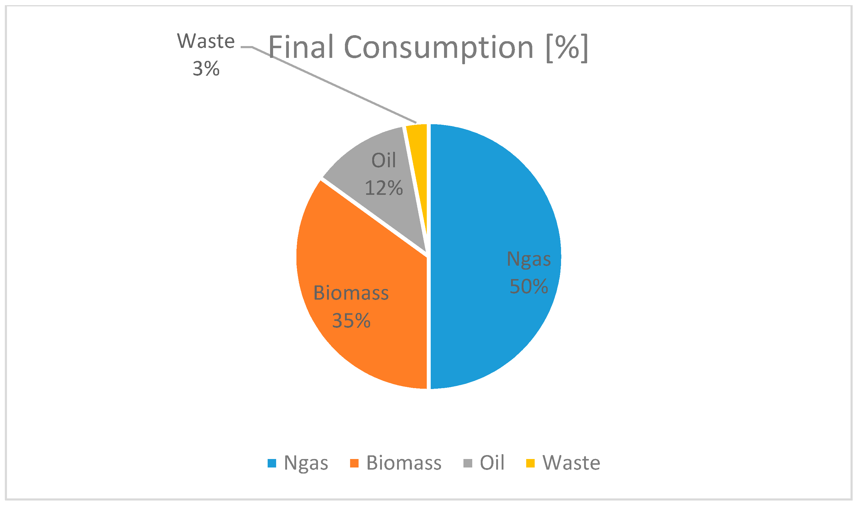
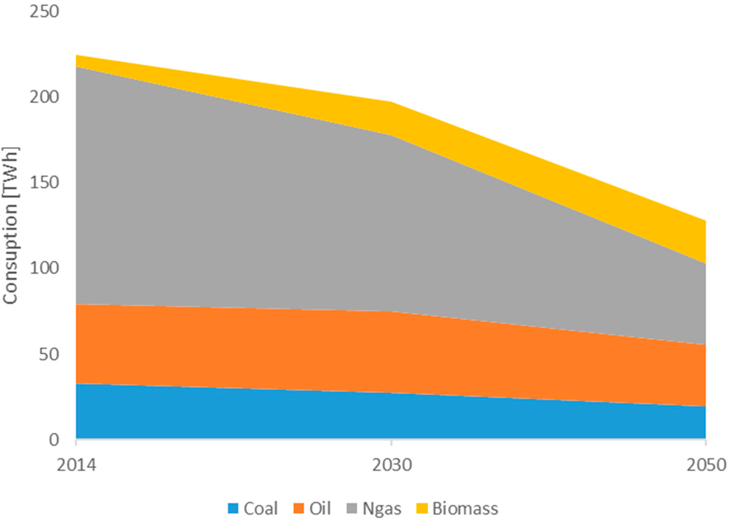
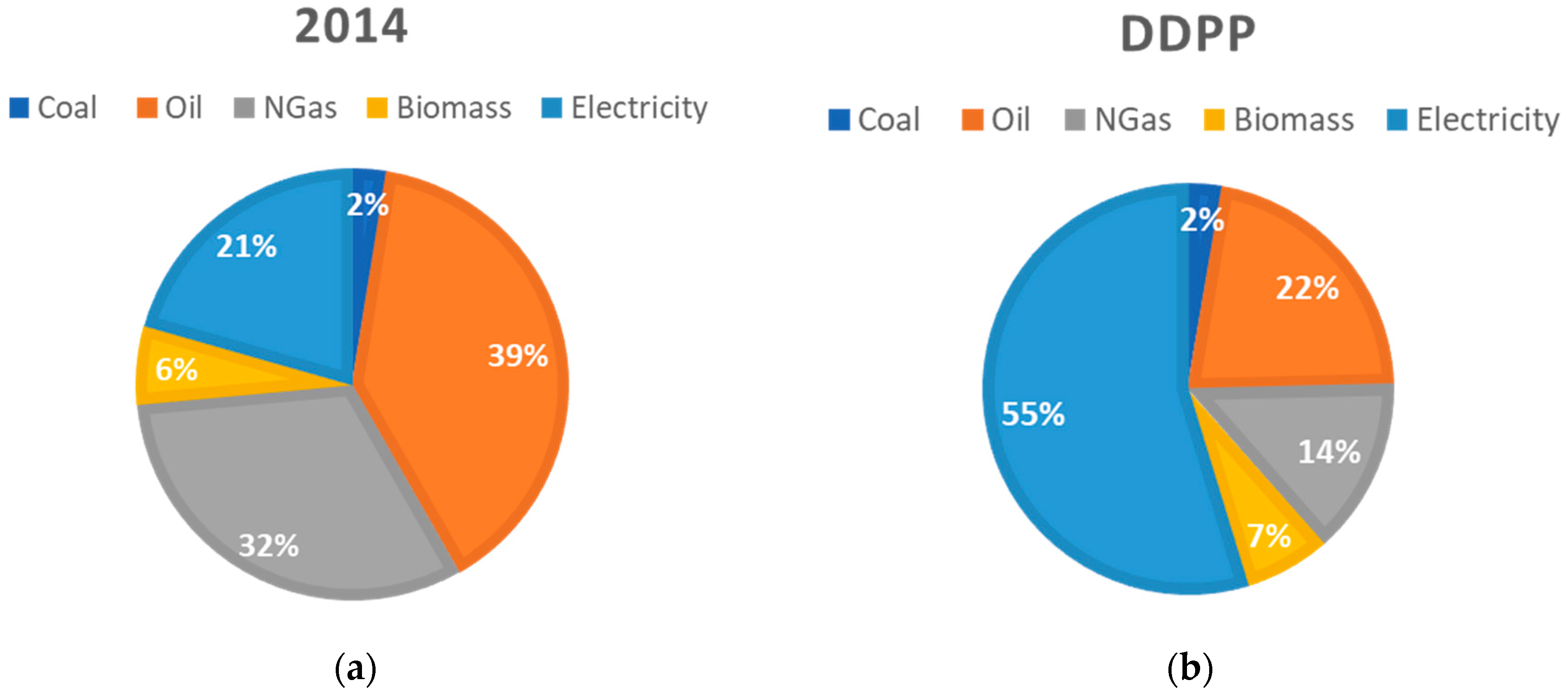
In the industrial sector, fossil fuel will be replaced by biomass and renewable energies. The use of coal and gas, as shown in Figure 10, will decrease, but the use of oil keeps constant.

Modal shift (from road to rail transport) and the spread of electric vehicles and plug-in hybrids will lead to an increase of electricity demand for transport. Electric vehicles and hybrids will represent, in 2050, 90% of road passenger transportation.

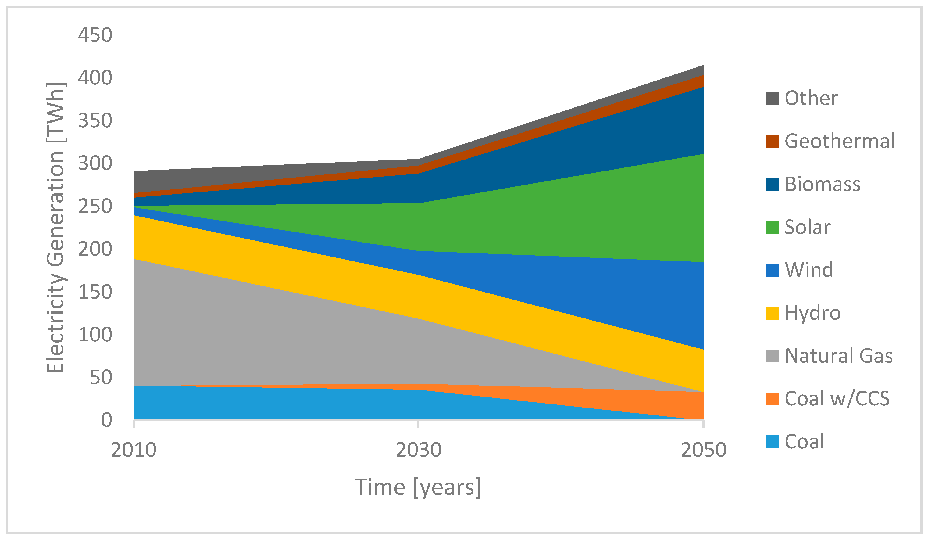
In line with European targets, the energy generation sector will have to change drastically to encourage the penetration of renewable energies. Total electric capacity of PP will be about the half of the present capacity. Instead, the installed CHP power will increase to 20 GW. Figure 11 shows the electricity generation trend by source in Italy.

The use of renewable resources envisioned in this scenario beholds an overall growth. Solar plant production represents the 24% of the renewable electricity production, with capacity installed of 55 GW. Concentrated solar power (CSP) with thermal storage allows the electricity production even six hours after sunset, providing an important input to solar generation (32 TWh).

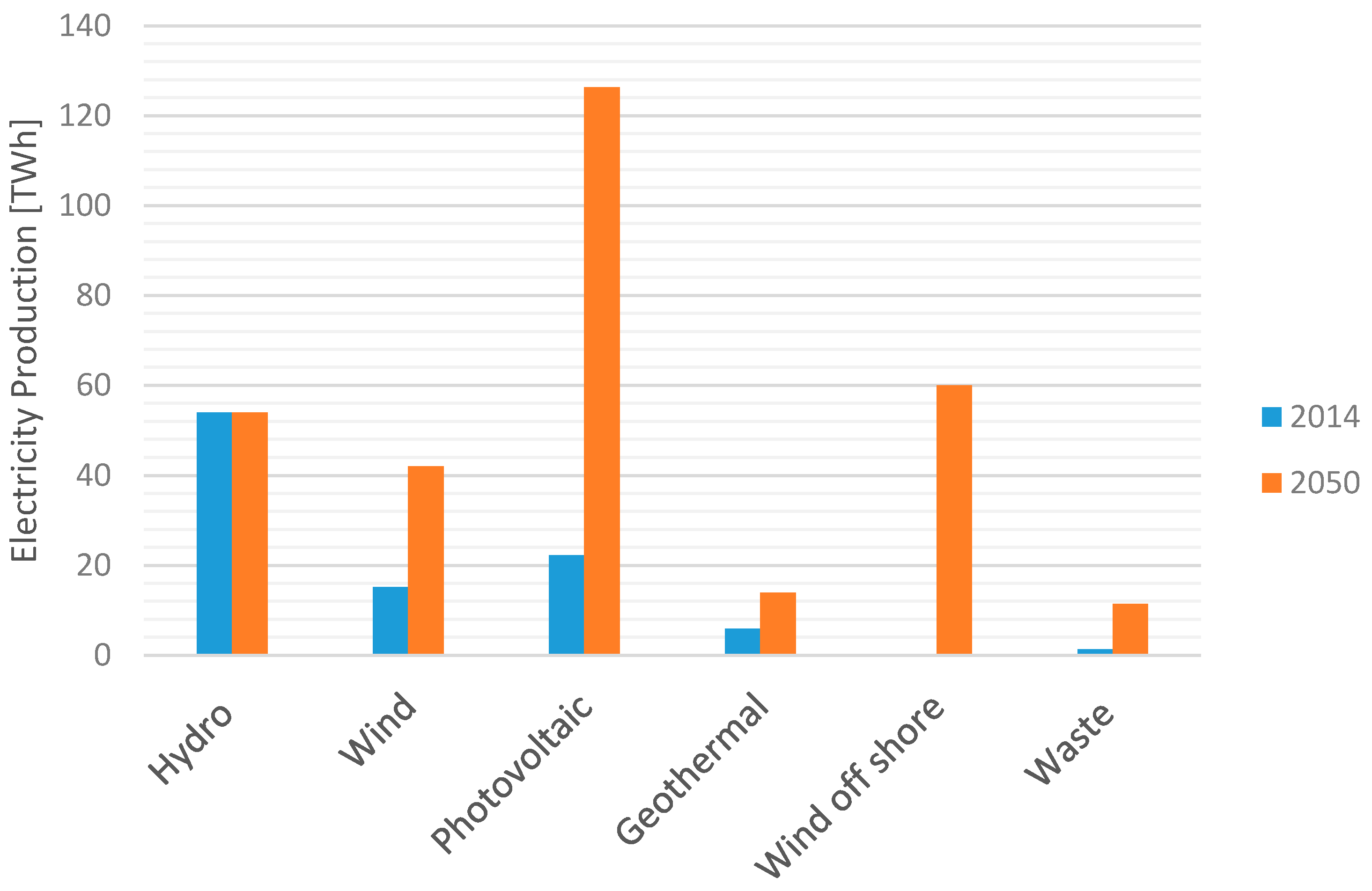
Wind turbines provide 11% of total renewable generation in 2050. Generation from offshore wind is even more important, amounting to 60 TWh. Hydro-power generation remains constant, because the level of exploitation of this source in Italy is already near to 100%.

This higher penetration of RES can create problems of reliability and sufficiency for traditional transmission grid; extensive investments will be required for developing smart grids, storage systems and hydrogen production. Figure 12 shows the difference in electricity production by renewable sources between 2014 and 2050 in the EFF scenario.

The reduction of emissions is the result of the diversification of energy sources. The EFF Scenario predicts that the only fuels used in power plants and CHP will be biomass and coal.

Waste-to-energy technologies could grow over the next 40 years, especially for district heating and cogeneration plants.

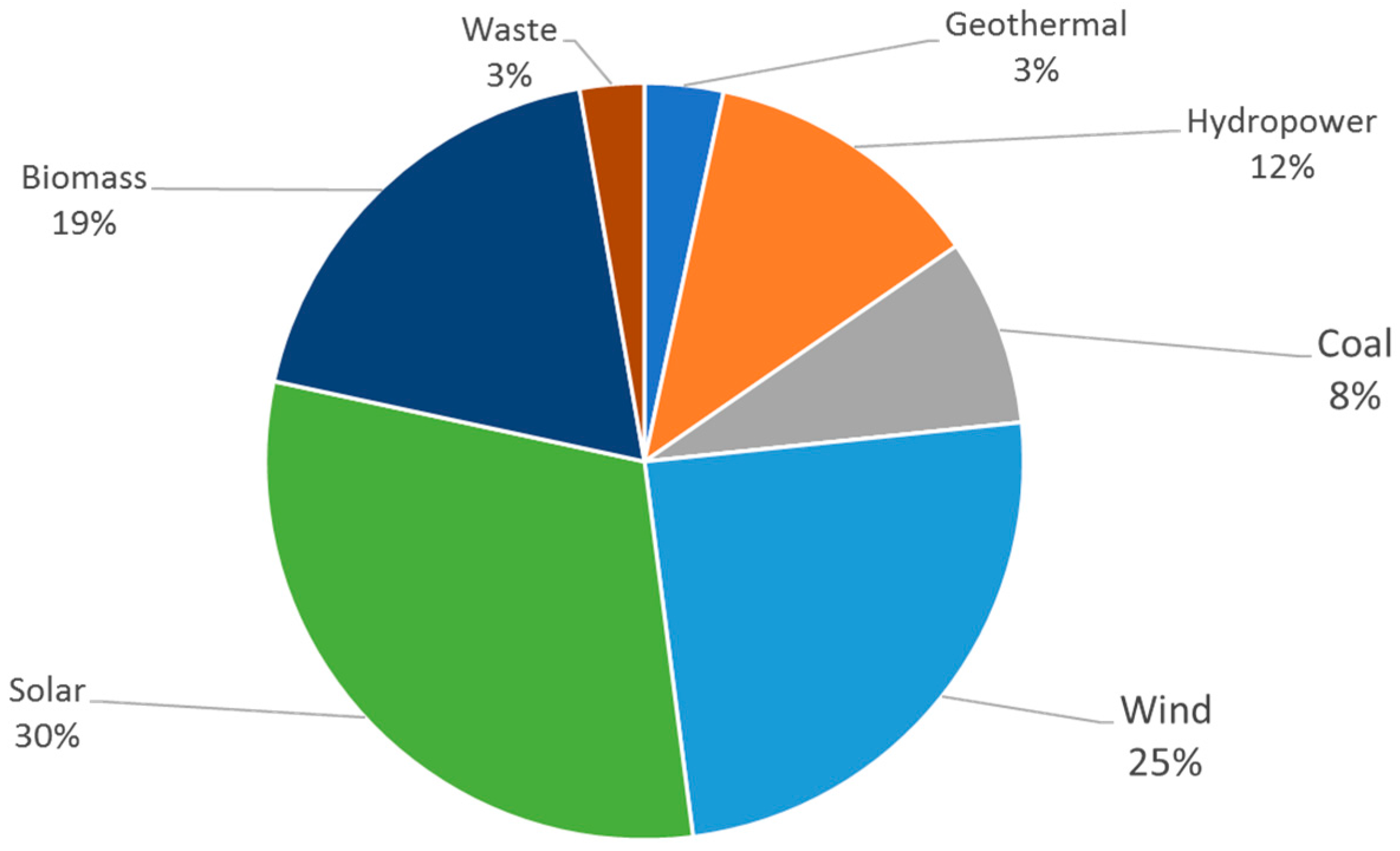
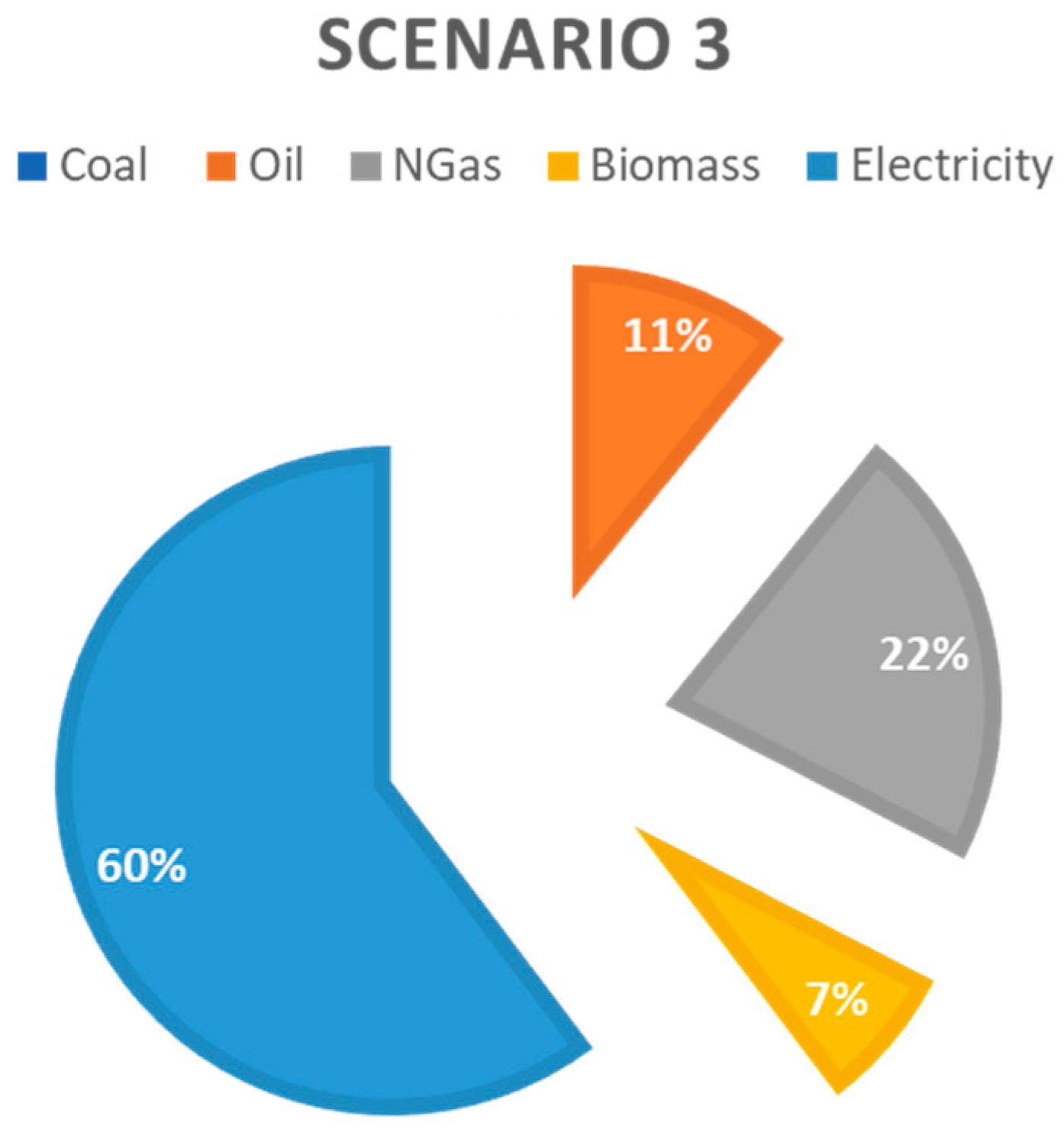
Figure 13 shows that, in percentage, the electricity production by source in 2050.

The EFF Scenario developed by ENEA predicts 81.6 Mt of CO₂ emissions in 2050.

However, a thorough analysis of this ENEA scenario shows some critical issues:

• the level of CEEP (critical excess electricity production) is very high: 43.19 TWh. This value is equal to the 22% of PV and wind production and higher than the recommended value of 5% [41];
• DH and DC cover a low percentage of the heating and cooling demands (respectively 17% and 0.04%);
• biomass consumption is too high for Italy (almost 301.8 TWh) and not sustainable, due to the limited availability of land, which is mainly used for farming, food, and other agricultural activities;
• the consumption of fossil fuels as coal and oil can be reduced, together with CO₂ emissions;
• the use of waste for energy production is too high, considering the increasing trend in recycling.

For these reasons, in the present study, three alternative scenarios were developed using critical excess electricity generation as optimization criteria, fuel consumption, and CO₂ emissions, which are, incidentally, the most employed optimization indicators in those studies that use EnergyPLAN simulations.

In fact, district heating and cooling can be increased to satisfy more than 50% of the demand, replacing both biomass boilers and heat pumps for individual heating. To meet the new district heating demand, the overall capacity would increase, together with the introduction of power-to-heat systems and thermal storage. Biomass consumption can be partially replaced by domestic natural gas sources in for PP and CHP. Biomass consumption for individual heating can decrease or be totally avoided when using more district heating. Waste input is set to a lower value, considering recycling trend.

To obtain a CEEP value under the 5% of RES production, vehicle-to-grid applications have been introduced.

Petrol and diesel consumption in the transport sector have been replaced in part with electricity and in part with alternative fuels (H₂ and synthetic fuel), whose production can also be useful to regulate the electric grid. It is assumed that the mileage remains the same as in 2014 (people’s behavior does not change). The capacity of a single battery is set equal to 50 kWh, more than in EFF scenario.

Coal and oil are replaced by biomass and natural gas in the industry and fuel sectors.

In the first alternative, the goal is a higher share of DH and DC, respectively meeting 50% of the total heat demand and 40% of total cooling demand. This objective can be achieved by a 30% increase of CHP installed capacity. Furthermore, the introduction of heat pumps (electric capacity of 6000 MW) in district heating plays a key role. This matches with 1 GW thermal storage for each GW of CHP installed capacity.

The second alternative presents a higher share of district heating and district cooling, higher installed capacity (CHP, RES, and heat pumps), solar thermal technology for DH (3 TWh), electrofuels in transport sector (4 TWh), and lower CCS technology capacity (10 Mt) with respect to DDPP Scenario (20 Mt). Furthermore, district heating is divided into two groups and the same thing is done for CHP that are divided into two groups. 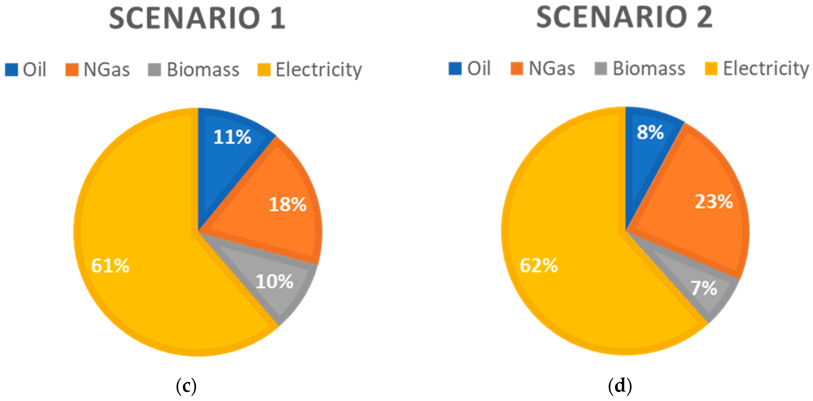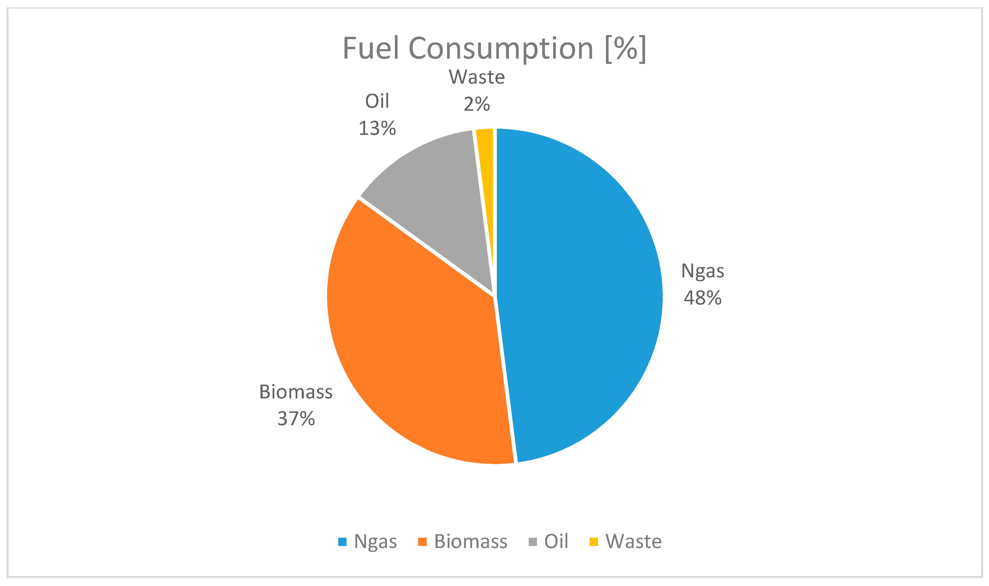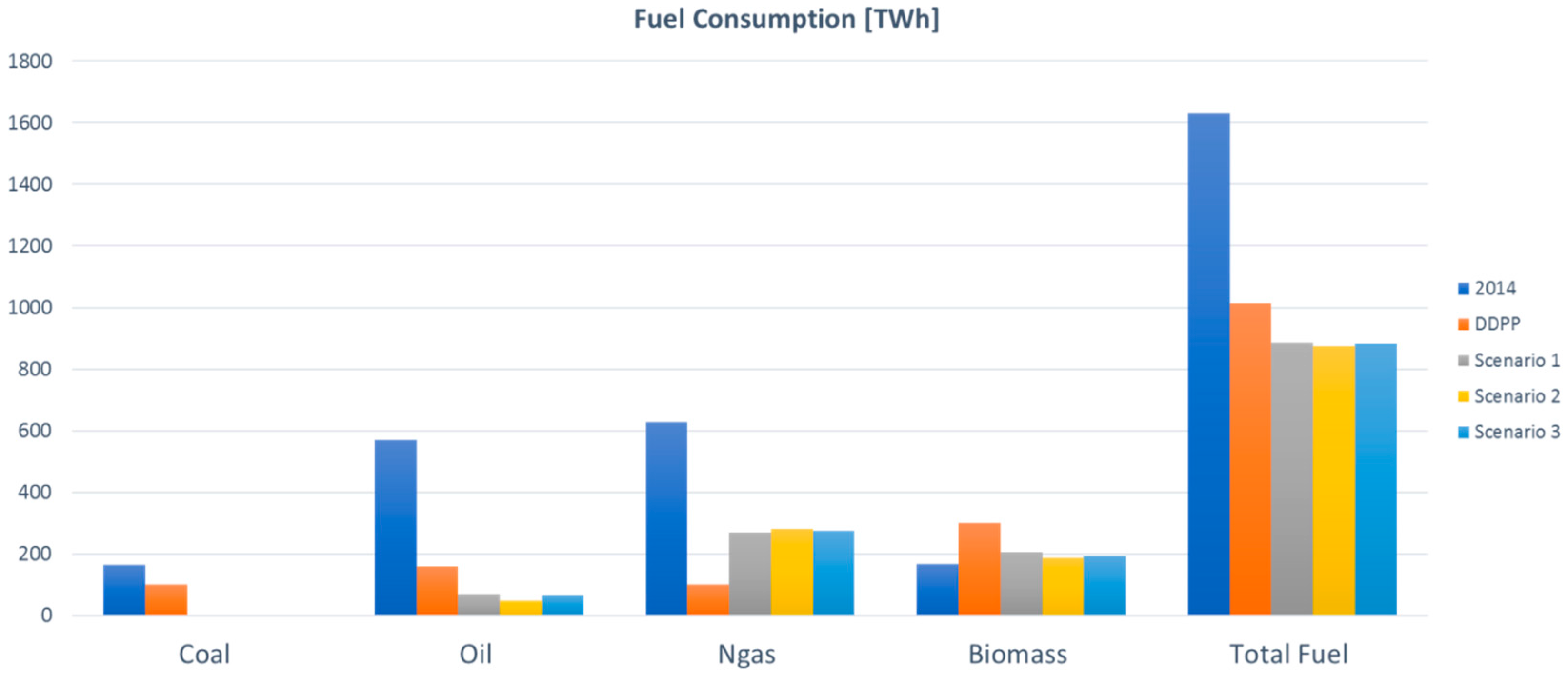Figure 14 and Figure 15 show the final fuel consumption by source respectively in the first and second alternative.

The results of Scenario 1 and Scenario 2 were compared and a third scenario was implemented, considering the best options between the two:

• district heating and district cooling are designed to meet 53% and 42% of heating and cooling demands, respectively;
• for CHP installed capacity, the best option is the one that presents the overall capacity in Group 3;
• CHP, compression heat pumps, and thermal storage capacity values are set to meet the heat demand in DH Group 3;
• the overall RES capacity is set to the DDPP (EFF Scenario) value;
• the CO₂ captured by CCS technology is set to 10 Mt.

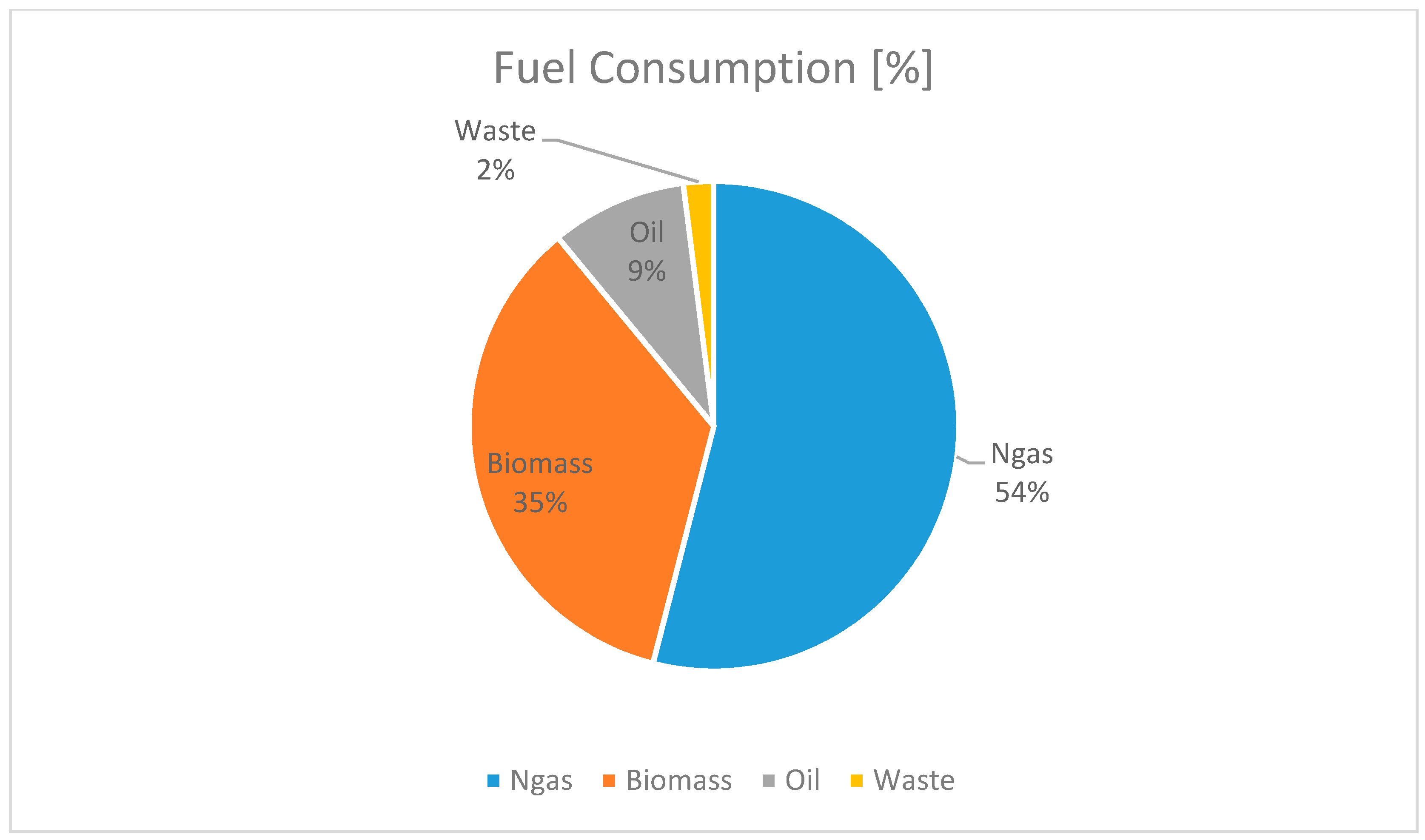
Figure 16 shows the final fuel consumption by source in the third alternative.

Table 9. Differences among scenarios for each field.

Fields	Year 2014	DDPP	Scenario 1	Scenario 2	Scenario 3
Power plant capacity (MW)	67,649	33,000	42,000	36,000	47,000
Small cogeneration plant capacity (MW)	2402	-	-	12,000	-
Big cogeneration plant capacity (MW)	16,674	20,000	40,000	35,000	44,000
Heating demand covered by district heating (%)	3	17	49	53	53
Cooling demand covered by district cooling (%)	0.4	0.4	37	42	42
Solar thermal production (TWh)	-	-	-	3	-
Thermal storage capacity (MWh)	-	-	39	66	42
Compression heat pumps capacity (MWe)	-	-	6000	7800	9750
Coal consumption (TWh/year)	165.66	101.8	0.22	-	0.22
Oil consumption (TWh/year)	571.38	158.4	70.5	50	67
Ngas consumption (TWh/year)	626.72	100	268.7	280	274.55
Biomass consumption (TWh/year)	169.04	301.8	204.2	187.7	194.02
Total fuel consumption (TWh/year)	1629	1014	885.2	874.2	881.55
CO2 (Mt)	337.66	78	54	60.8	64.4
CEEP [%]	-	22	1.13	4.6	0.02
RES share in electricity production [%]	40	104	90	91.9	90.1

shows the inputs and the results obtained for each scenario, in each field. The results and the differences among these scenarios are shown in Figure 17 and Figure 18.

In Figure 19, it is possible to see the different energy mix for all scenarios.

6. Conclusions

This paper aims at providing a profound analysis of the feasibility of Italian decarbonization targets, presenting different alternative pathways to reduce by at least 80% of GHG emissions by 2050, with respect to 1990.

In the analysis of these energy scenarios, it emerged that to achieve the deep decarbonization goals a drastic transition is needed. This transition is based on a shift from traditional energy systems, with electricity needs mainly covered by conventional power plants, transport demands mainly covered by petrol and diesel and heating demands mainly covered by individual boilers, to energy systems in which: (i) the electricity needs are covered by solar and wind power, combined with biomass-fueled CHP plants; (ii) transportation demand is fulfilled by synthetic fuels produced by electrolytic converters; (iii) heat is supplied from heat pumps, CHP plants and waste-to-heat technologies. All the alternative future scenarios show these main characteristics: the RES share for electricity production is above 90% with respect to 40% in 2014; the introduction of electrofuels and a modal shift bringing a reduction of 60% in fossil fuel consumption; district heating and district cooling cover around 50% and 40% of the residential heating and cooling total demand, respectively. These actions lead to a CO₂ emissions reduction of over 82% with respect to 2014 level and over 85% with respect to 1990 level, a TFC reduction around 50% with biomass consumption at the same level of 2014 in line with the EU action plan for a low carbon economy. It is clearly shown how in each alternative future decarbonization target scenario, already contemplated in the DDPP scenario, are fulfilled and exceeded. In fact, the CO₂ emissions in alternative scenarios present a reduction with respect to DDPP scenario level that goes from 18% to 31%, while the TFC reduction is around 13%. In addition to the decarbonization objectives, the alternative scenarios show a higher economic sustainability (%CEEP under the recommended value of 5%, with respect to 22% of DDPP scenario) and environmental sustainability with a reduction of around 30% in biomass consumption.

A strong decrease in the carbon intensity of energy is required. Renewable sources and a strong electrification of heating and transport services should progressively replace fossil fuel consumption.

The success of the DD (degree days) will strongly rely on the development of solar and wind (especially offshore) technologies, a significant contribution is also expected from biomass and district heating. Such technologies are largely available on the market and their penetration is definitely possible in Italy, as seen in recent years.

The cost of most technologies for renewables and energy efficiency have been decreasing, and both wind and solar PV are close to grid-parity with traditional options.

One of the major technical difficulties will be the management of variable renewable energy sources.

In fact, one common characteristic of many transitions is the shift from a relatively limited number of storable fuels towards many fluctuating and complementary energy sources.

This requires the modernization of the electric grid, which can be achieved by increasing the interconnection of market zones and installing storage systems.

The development of fast-charging infrastructure for electric vehicles would help stabilizing the grid during the peak RES generation.

Another issue is whether biomass could cover between 16% and 19% of electricity generation. The sustainability of such production must be investigated to avoid negative environmental and economic impacts.

Regarding energy policies, Italy adopted several measures to support the development of RES and the increase of energy-efficiency (green certificates, feed-in tariffs, investment subsidies, tax deductions, etc.). However, stronger efforts are needed to achieve the 2050 targets and modernization of the Italian energy system.

Considering the limited public financial budgets, the major challenge is to involve the private sector for financing the energy transition process.

A common critique to the Italian approach is the lack of a national industrial development strategy.

Finally, public engagement initiatives for involving citizens and local communities in the decision process is a key element to achieve a larger social acceptance of many renewable technologies and projects.