Research on Risk Evaluation of Transnational Power Networking Projects Based on the Matter-Element Extension Theory and Granular Computing

Abstract
:1. Introduction
- A risk evaluation index system and the corresponding judging criteria of transnational networking projects are established in this paper. Based on the characteristics of transnational networking projects, a comprehensive risk evaluation index system, including four first-level indicators and eleven secondary indicators, and the corresponding judging criteria are established.
- The Global Peace Index and the National Governance Index are employed during the quantization of the related qualitative indexes. The Global Peace Index and the National Governance Index are respectively introduced in this paper during the quantization of “War or terrorist attack” and “Change of government or statute”, which are two important qualitative indicators in the index system.
- A combination weighting method is proposed in the weight determination part. This paper employs a combination of granular computing and the order relation analysis method to determine the weight of each indicator, aiming at improving the reliability of the results, which can finally help to improve the rationality of the evaluation result.
2. Method
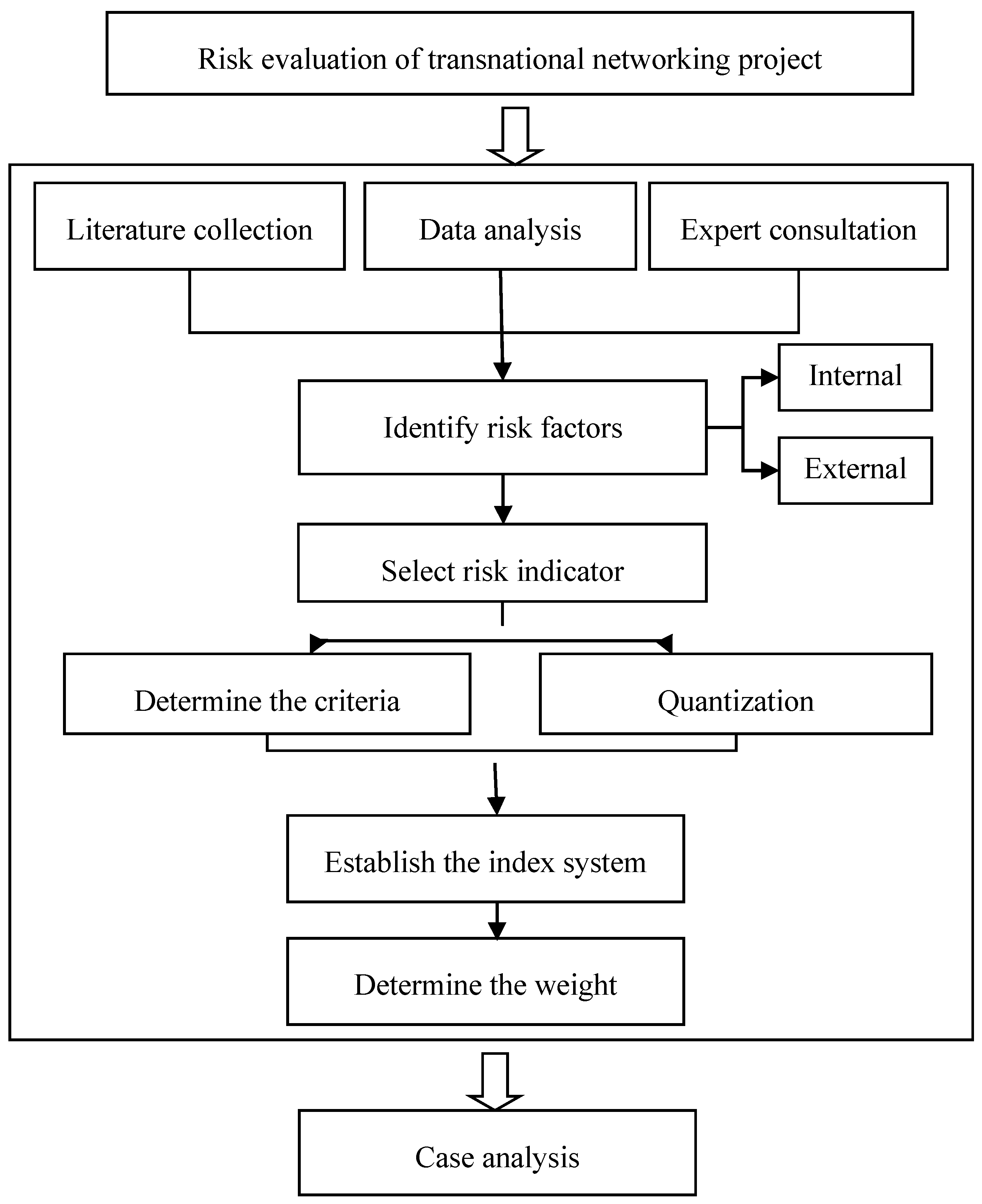
2.1. Research Procedure
2.2. Weight Determination
- Step 1:
- Providing the index system and the evaluation criteria for the experts. All members of the expert group will assign a mark to each index independently to indicate the importance of each indicator. Suppose there are “n” experts and “m” indicators, the original data “X” can be obtained, where X = {x1, x2, ..., xn}, xi = {yi1, yi2, ..., yim}, i = 1, 2, ..., n.
- Step 2:
- Calculating the similarity relation between xi and xj, where i and j represent different experts. Then, as shown in Equation (1), the fuzzy similarity matrix of the samples can be obtained:
- Step 3:
- The quotient space family with inclusion relation, , can be calculated and different values of stand for different granular spaces.
- Step 4:
- Calculating the importance of each index in different granular spaces. The importance can be gained by:where is the kth indicator; C is the condition attribute set; D is the decision attribution set; stands for the condition attribute set’s dependence on decision index set when the is dropped from C.
- Step 5:
- The comprehensive importance can be calculated by Equation (3):where q is the number of total quotient space families; is the importance of in the quotient space family of X().
- Step 1:
- Obtaining the order relation. According to the available information, experts give marks to the indicators based on his own experience, the original order relation can be obtained as follows:where x represents different indicators; m is the number of the indicator.
- Step 2:
- Calculating the importance ratio. On basis of the order relation obtained in step 1, the importance ratio of two adjacent indicators can be calculated according to the original marks provided by the expert:where refers to the kth importance ratio; wk−1 is the score of the (k − 1)th indicator; wk is the score of the kth indicator.
- Step 3:
- Determining the weight of each indicator:where is the weight of the kth indicator determined by the G1 method.
- Step 4:
- Results integration. Differences may exist between the weights determined by different experts and it is essential to make a comprehensive analysis of the results obtained from different experts. The final result of the weight can be calculated by:where L is the number of the expert; is the final weight of the kth indicator.
2.3. Matter-Element Extension Evaluation Model
- Step 1:
- Determine the classical domain, joint domain and the object to be evaluated:where stands for the jth grade of the matter-element model; represents the jth grade of the object in classical domain; c1, ..., cn are the features of Nj; Vji and are the range of ci under the jth grade, i = 1, 2, ..., n (Classical domain):where p stands for the level of the object to be evaluated; vpi and are the range of ci under all grades, i = 1, 2, ..., n (Joint domain):where p0 is the object to be evaluated; vi is the observed value of indicator ci, i = 1, 2, ..., n.
- Step 2:
- Obtain the weight of indicator. This paper employs a combination of granular computing and G1 Method to determine the weight of each indicator.
- Step 3:
- Normalization. The way of normalization is shown in Equations (12) and (13):
- Step 4:
- Calculate the correlation degree:where D is the distance from the object to the classical domain; K is the correlation degree, i = 1, 2, ..., n.
- Step 5:
- Draw the conclusions. According to the principle of maximum relevance, the level of the object to be evaluated can be determined based on the results obtained in Step 4.
3. Index System
3.1. Political Risk
3.2. Social and Natural Risk
3.3. Economic Risk
3.4. Technical Risk
4. Case Study
4.1. Basic Information of the Project to Be Evaluated
4.2. Weight Determination
- Step 1:
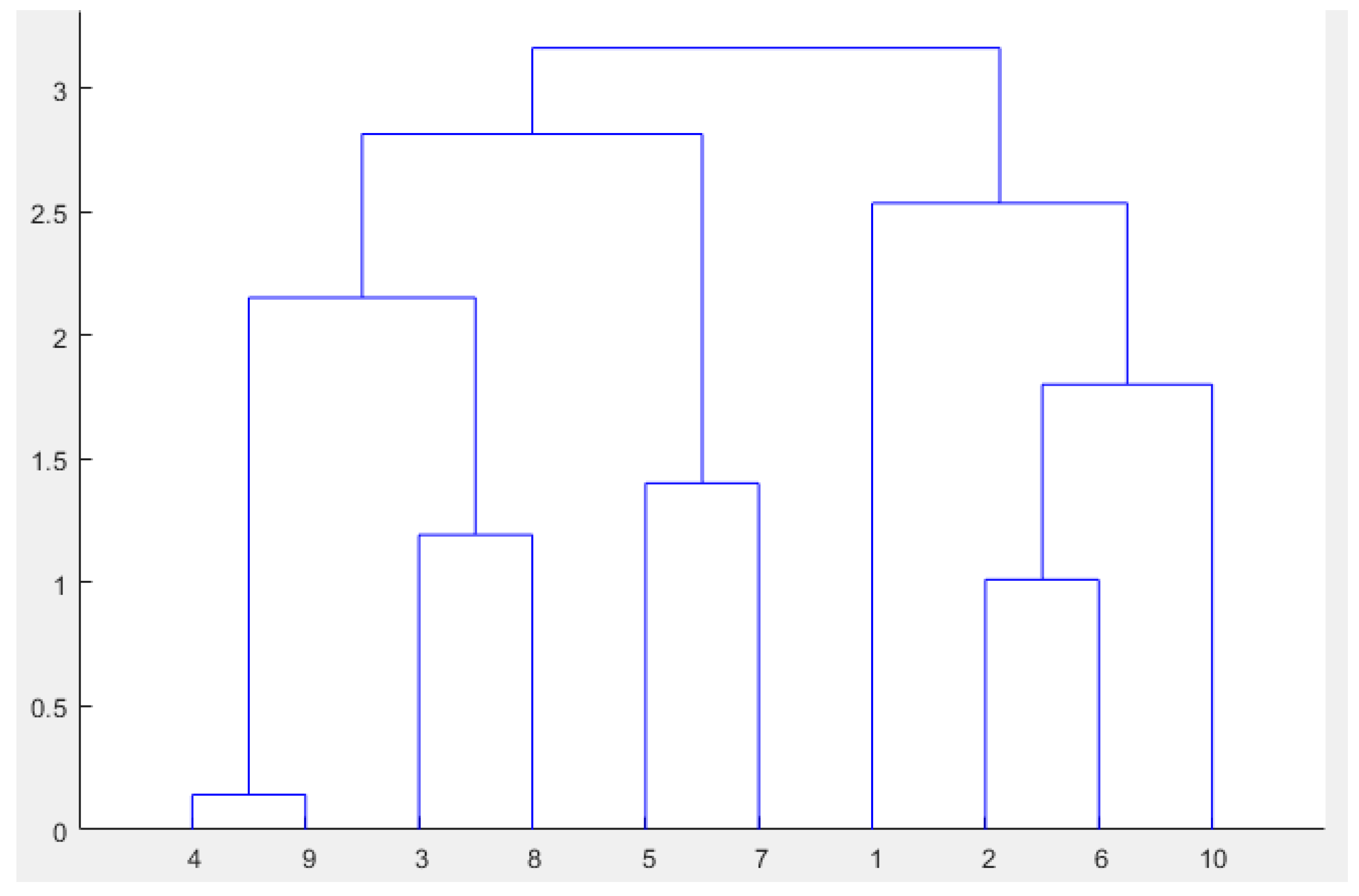
- Standardizing the original data. According to the scores of the first-level indicators, distance between different samples can be calculated by using the MATLAB. Different kinds of distance between classes, including “ward”, “complete”, “average”, “centroid” and “single”, are employed for clustering according to the characteristics of the original data. Then, the composite coefficient “Q” can be calculated to determine the optimal distance between classes, and the closer Q is to 1, the better the clustering is. The composite coefficient of first-level indicators can be calculated by using MATLAB and the results are as follows: Q = {0.8355, 0.8501, 0.8607, 0.7960, 0.7692}. The maximum value of Q is “0.8607”, which means the distance of “average” between classes is much more appropriate (the distance between samples is Euclidean distance). The result of clustering is shown in Figure 2, and the families of quotient space can also be obtained according to the clustering result (shown in Table 10).
- Step 2:
- The discrete interval provided by the expert group is applied in data discretization and then, the corresponding equivalence class can be obtained when one of the indexes is deleted:U/ind (S-{A}) = [{x1},{x2},{x3},{x4},{x5},{x6,x9,x10},{x7},{x8}]U/ind (S-{B}) = [{x1,x4},{x2,x6,x10},{x3},{x5},{x7},{x8},{x9}]U/ind (S-{C}) = [{x1},{x2},{x3},{x4},{x5},{x6,x7,x9,x10},{x8}]U/ind (S-{D}) = [{x1},{x2},{x3},{x4,x7},{x6,x10},{x8},{x9}]
- Step 3:
- On the basis of the results obtained above, the importance of each first-level index in different granularity spaces can be calculated and at the same time, the weight of first-level indicators can be determined after normalization. Table 11 shows the attribute significance and the weight of the first-level index.
- Step 4:
- Calculation of the weight of the secondary indicators. The process of determining the weight of secondary indexes by granular computing is the same as the steps above, and due to the length limitation, no more details will be repeated. Table 12 shows the weight of indicators obtained by using granular computing.
- Step 1:
- Determining the order relation. The order of first-level indexes can be obtained in the light of the scoring results.
- Step 2:
- Calculating the importance of each index. For example, an order of the four first-level indexes can be determined according to expert’s scores: BDCA. “R” represents the relative importance of two adjacent indicators, and then a series of results can be calculated according to the original data: R2 = A/C = 1.12, R3 = C/D=1.06, R4 = D/B = 1.11; w(B) = 1/(1 + R2 × R3 × R4 + R3 × R4 + R4) = 0.217, w(D) = 0.217 × 1.11 = 0.241, w(C) = 0.241 × 1.06 = 0.256, w(A) = 0.256 × 1.12 = 0.286.
- Step 3:
- Repeating the previous steps to gain the weight determined by all experts. Each expert will determine an order relation between the first-level indicators according to their own experience, and it is necessary to repeat the steps above to obtain the weights determined by different experts.
- Step 4:
- Obtaining the comprehensive weight of the first-level indicator. The comprehensive weight can be obtained directly by seeking the arithmetic mean of the data obtained in Step 3. And the results are as follows:w(A) = 0.258, w(B) = 0.237, w(C) = 0.249, w(D) = 0.256.
- Step 5:
- Repeating the steps above to gain the weight of each secondary indicator. And the weights calculated by G1 Method are listed in Table 13.
4.3. Risk Evaluation of Two Investment Schemes
- (1)
- Classifying the risk level of the system. In this paper, the risk level of the transnational HVDC transmission project is divided into five different grades, including “Extremely Low”, “Low”, “General”, “High” and “Extremely High”.
- (2)
- Determining the classical domain of each index. The classical domain of each indicator is listed as follows (except indicator “B1”): the classical domain of “Extremely Low” is (0,0.2); “Low” is (0.2,0.4); “General” is (0.4,0.6); “High” is (0.6,0.8); “Extremely High” is (0.8,1). The classical domain of different risk levels and the matter-element to be evaluated are shown as follows:where R represents the classical domain of five different risk levels; N stands for the different risk level; R′ and R″ represent the matter-element to be evaluated.
- (3)
- Determining the weight of each indicator. Utilizing the weights obtained above, the final comprehensive weight of each secondary indicator can be calculated by synthesizing the results obtained in Section 4.2., which can effectively improve the rationality of the final result. The final comprehensive weight is listed in Table 14.
- (4)
- (5)
- Computing the correlation degree. According to the results obtained above, the correlation degree of two schemes with different risk levels can be calculated, respectively.The correlation degree of R′ (Table 15, Scheme 1):The correlation degree of R″ (Table 15, Scheme 2):
- (6)
- Determining the risk level. According to the correlation degree calculated above, the comprehensive risk level of two investment schemes can be determined: the risk level of Scheme 1 is “Low” since K2 is the maximum value among the five correlation degrees of R′; the risk level of Scheme 2 is “General” because K3 is the maximum value among the five correlation degrees of R″.
4.4. Analysis of the Evaluation Result
5. Conclusions
Acknowledgments
Author Contributions
Conflicts of Interest
References
- General Office of the State Council. Available online: http://www.gov.cn/zhengce/content/2014-11/19/content_9222.htm (accessed on 1 March 2017).
- National Development and Reform Commission, National Energy Administration. Available online: http://www.chinapower.com.cn (accessed on 1 March 2017).
- CPC Central Committee and the State Council. Available online: http://www.cec.org.cn (accessed on 2 March 2017).
- Polaris Smart Grid Online. Available online: http://news.bjx.com.cn (accessed on 2 March 2017).
- Polaris Smart Grid Online. Available online: http://news.bjx.com.cn/html/20100126/241904.shtml (accessed on 2 March 2017).
- Eissa, M.A.; Tian, B. Lobatto-Milstein Numerical Method in Application of Uncertainty Investment of Solar Power Projects. Energies 2017, 10, 43. [Google Scholar] [CrossRef]
- Muriana, C.; Vizzini, G. Project risk management: A deterministic quantitative technique for assessment and mitigation. Int. J. Proj. Manag. 2017, 35, 320–340. [Google Scholar] [CrossRef]
- Zhao, H.; Guo, S. Risk Evaluation on UHV Power Transmission Construction Project Based on AHP and FCE Method. Math. Probl. Eng. 2014, 1, 1–14. [Google Scholar] [CrossRef]
- Kang, H.Y.; Lee, A.H.; Huang, T.T. Project Management for a Wind Turbine Construction by Applying Fuzzy Multiple Objective Linear Programming Models. Energies 2016, 9, 1060. [Google Scholar] [CrossRef]
- Fu, W.X. Risk Assessment and Control of Wenzhou Power Grid Construction Project. Master’s Thesis, Zhejiang University, Zhejiang, China, 2010. [Google Scholar]
- Wang, Q. Research on Risk Assessment Method of Power Grid Construction Based on EPC Mode. Master’s Thesis, North China Electric Power University, Beijing, China, 2015. [Google Scholar]
- Long, R.; Zhang, J. Risk Assessment Method of UHV AC/DC Power System under Serious Disasters. Energies 2017, 10, 13. [Google Scholar] [CrossRef]
- Yang, L. The evaluation of political risk in transnational investment. Technol. Entrep. Mon. 2008, 04, 35–37. [Google Scholar] [CrossRef]
- Wang, D.J.; Li, X.S. Strategic risk assessment of transnational oil and gas investment based on Scenario Planning. J. China Univ. Pet. (Nat. Sci. Ed.) 2012, 2, 191–195. [Google Scholar] [CrossRef]
- Zhang, Y.X.; Xu, C.Y.; Cheng, J.H. Price risk assessment of Chinese petroleum enterprises’ cross border mergers and acquisitions based on VaR method. J. Manag. 2010, 3, 440–444. [Google Scholar] [CrossRef]
- Jin, X.H. Determinants of Efficient Risk Allocation in Privately Financed Public Infrastructure Projects in Australia. J. Constr. Eng. Manag. 2009, 136, 138–150. [Google Scholar] [CrossRef]
- Li, J.; Zou, P.X. Fuzzy AHP-Based Risk Assessment Methodology for PPP Projects. J. Constr. Eng. Manag. 2011, 137, 1205–1209. [Google Scholar] [CrossRef]
- He, Y.X.; Dai, A.Y.; Yang, W.H.; Luo, T.; Liu, B.R. Research on risk assessment of urban power network planning based on extension analysis and matter element model. J. North China Electr. Power Univ. (Nat. Sci. Ed.) 2010, 6, 6–11. [Google Scholar] [CrossRef]
- Wu, Q.L.; Peng, C.Y. Comprehensive Benefit Evaluation of the Power Distribution Network Planning Project Based on Improved IAHP and Multi-Level Extension Assessment Method. Sustainability 2016, 8, 796. [Google Scholar] [CrossRef]
- Sun, X.L.; Chu, J.D.; Ma, H.Q.; Cao, S.L. Improvement and application of matter element extension evaluation method. Hydrology 2007, 1, 4–7. [Google Scholar] [CrossRef]
- Xu, X.M.; Niu, D.X.; Qiu, J.P.; Wu, M.Q.; Wang, P.; Qian, W.Y.; Jin, X. Comprehensive Evaluation of Coordination Development for Regional Power Grid and Renewable Energy Power Supply Based on Improved Matter Element Extension and TOPSIS Method for Sustainability. Sustainability 2016, 8, 143. [Google Scholar] [CrossRef]
- Qin, S.K. Principle and Application of Comprehensive Evaluation, 1st ed.; Publishing House of Electronics Industry: Beijing, China, 2003; pp. 9–11. [Google Scholar]
- Zadeh, L.A. Fuzzy Sets and Information Granularity. In Fuzzy Sets, Fuzzy Logic, and Fuzzy Systems: Selected Papers by Lotfi A. Zadeh; World Scientific Publishing Co., Inc.: River Edge, NJ, USA, 1979; pp. 433–448. [Google Scholar]
- Zhou, D.C. Method for determining attribute weights by Granular Computing. J. Intell. Syst. 2015, 2, 273–280. [Google Scholar] [CrossRef]
- Cai, W. The summary of extension theory. Syst. Eng. Theory Pract. 1998, 18, 76. [Google Scholar] [CrossRef]
- He, Y.X. Comprehensive Evaluation Method and Application of Electric Power, 1st ed.; China Electric Power Press: Beijing, China, 2011; pp. 96–112. ISBN 9787512319691. [Google Scholar]
- Li, H.Z.; Guo, S.; Tang, H.; Li, C.J. Comprehensive Evaluation on Power Quality Based on Improved Matter-Element Extension Model with Variable Weight. Power Syst. Technol. 2013, 37, 653–659. [Google Scholar]
- Wu, C.K. A New Approach to the Study China’s National Defense and Borderland Defense. J. Yunan Norm. Univ. (Philos. Soc. Sci. Ed.) 2010, 42, 1–7. [Google Scholar] [CrossRef]
- Sun, W.; Li, J.Y. Technological Economics, 1st ed.; Machinery Industry Press: Beijing, China, 2011; pp. 51–53. [Google Scholar]
- NDRC. The Pre-Tax Financial Benchmark Rate of Return on Investment of Construction Projects in China; National Development and Reform Commission; Ministry of Construction, People´s Republic of China: Beijing, China, 2006.
- Pan, X.J.; Lin, Y.Z. Research on the influence of exchange rate on international project. Constr. Econ. 2011, S1, 10–12. [Google Scholar] [CrossRef]
- Kaiser, B.; Siegenthaler, M. The skill-biased effects of exchange rate fluctuations. Econ. J. 2016, 126, 756–780. [Google Scholar] [CrossRef]
- Liu, W.; Yang, H.X.; Zhu, B. Review of technical standards system for smart grid. Power Syst. Prot. Control 2012, 10, 120–126. [Google Scholar] [CrossRef]
- CEC. Technical Specification for Evaluating the Effect of New Urbanization Power Grid Construction and Transformation; China Electricity Council: Beijing China, 2016. [Google Scholar]
- Zhai, H.J.; Fan, H.R.; Geng, Q.S. Research on economic evaluation and risk prevention of transnational HVDC project. J. North China Electr. Power Univ. (Soc. Sci.) 2016, 2, 23–26. [Google Scholar] [CrossRef]


| Year | Project | Status |
|---|---|---|
| 2015 | The 500 kV HVDC project between Thailand and China | In Planning |
| 2015 | The 500 kV HVDC project between Vietnam and China | In Planning |
| 2015 | China State Grid’s Extra High Voltage (EHV) projects plan based on the Belt and Road Initiative (Transmission corridor along the Silk Road economic belt) | In Planning |
| 2016 | The 500 kV Direct Current (DC) networking project between Ethiopia and Kenya | Under Construction |
| 2016 | The ±250 kV DC networking project between Malaysia and Indonesia | Under Construction |
| 2016 | The 400 kV Alternating Current (AC) networking project between Nepal and India | Under Construction |
| 2016 | Northeast Asia power interconnection project | Under Preparation |
| Method | Advantages | Disadvantages |
|---|---|---|
| Expert evaluation method |
|
|
| AHP |
|
|
| Fuzzy synthetic evaluation method |
|
|
| ANP |
|
|
| The Monte Carlo method |
|
|
| First-Level Indicator | Secondary Indicator |
|---|---|
| Political Risk (A) | State relation (A1) War or terrorist attack (A2) Change of government or statute (A3) |
| Social and Natural Risk (B) | Public acceptance (B1) Extreme weather or natural disaster (B2) |
| Economic Risk (C) | Net present value rate (C1) Internal rate of return (C2) Exchange fluctuations (C3) |
| Technical Risk (D) | Parameters of power network (D1) Reliability of power supply (D2) Construction risk (D3) |
| Index | Criteria and the Score | |||||
|---|---|---|---|---|---|---|
| A1 | Type Score | Union (0,2] | Strategic Partnership (2,4] | Partnership (4,6] | Friendship (6,8] | Diplomatic Relations (8,10] |
| Rank | Extremely Low | Low | General | High | Extremely High | |
| A2 | Score | (0,2] | (2,4] | (4,6] | (6,8] | (8,10] |
| Rank | Extremely Low | Low | General | High | Extremely High | |
| A3 | Score | (0,2] | (2,4] | (4,6] | (6,8] | (8,10] |
| Rank | Extremely Low | Low | General | High | Extremely High | |
| Index | Criteria and the Score | |||||
|---|---|---|---|---|---|---|
| B1 | Acceptance | 100% ≤ PA < 90% | 90% ≤ PA < 80% | 80% ≤ PA <6 0% | 60% ≤ PA < 40% | 40% ≤ PA ≤ 0% |
| Score | (0,2] | (2,4] | (4,6] | (6,8] | (8,10] | |
| B2 | Rank | Extremely Low | Low | General | High | Extremely High |
| Score | (0,2] | (2,4] | (4,6] | (6,8] | (8,10] | |
| Rank | Extremely Low | Low | General | High | Extremely High | |
| Index | Criteria and the Score | ||||||
|---|---|---|---|---|---|---|---|
| C1 | NPVR | NPVR ≥ 0 | NPVR < 0 | ||||
| Score | (0,6] | (6,10] | |||||
| Rank | Acceptable | Unacceptable | |||||
| C2 | IRR | IRR ≥ 7% | IRR < 7% | ||||
| Score | (0,6] | (6,10] | |||||
| Rank | Acceptable | Unacceptable | |||||
| C3 | Range | 0 ≤ F < 1% | 1% ≤ F < 2% | 2% ≤ F < 3% | 3% ≤ F < 5% | 5% ≤ F < 10% | |
| Score | (0,2] | (2,4] | (4,6] | (6,8] | (8,10] | ||
| Rank | Extremely Low | Low | General | High | Extremely High | ||
| Index | Criteria and the Score | |||||
|---|---|---|---|---|---|---|
| D | Score | (0,2] | (2,4] | (4,6] | (6,8] | (8,10] |
| Rank | Extremely Low | Low | General | High | Extremely High | |
| Item | Scheme 1 | Scheme 2 |
|---|---|---|
| Total investment (Million USD) | 4471.80 | 3095.81 |
| Project life cycle | 28 years | 28 years |
| Transmission line capacity | 8000 MW | 4400 MW |
| Voltage level | ±800 kV | ±660 kV |
| Cable type | 6 × 1250 mm2 | 6 × 720 mm2 |
| Annual Transmitted Power | 35,449 GWh | 35,449 GWh |
| Interruption time/Observation time | 0.0144 h/1000 h | 0.0352 h/1000 h |
| On-grid price (Supply-side) | 47.23 USD/MWh | 47.23 USD/MWh |
| Free on board | 51.89 USD/MWh | 51.02 USD/MWh |
| On-grid price (Receive-side) | 68.0 USD/MWh | 68.0 USD/MWh |
| Net present value of the project (Million USD) | 3092.76 | 3715.77 |
| Net present value rate (NPVR) | 73.6% | 97.4% |
| Internal rate of return (IRR) | 12% | 13.55% |
| Public acceptance | 78% | 65% |
| Benchmark yield | 7% | |
| Composite depreciation rate | 4.46% | |
| Import value-added tax | 8.5% | |
| Indicator | Scheme 1 | Scheme 2 | ||
|---|---|---|---|---|
| Ob | St | Ob | St | |
| A1 (State relation) | 3 | 0.3 | 3 | 0.3 |
| A2 (War or terrorist attack) | 3.9 | 0.39 | 3.9 | 0.39 |
| A3 (Change of government or statute) | 5.3 | 0.53 | 5.3 | 0.53 |
| B1 (Public acceptance) | 78% | 0.22 | 65% | 0.35 |
| B2 (Extreme weather or natural disaster) | 4.5 | 0.45 | 4.5 | 0.45 |
| C1 (NPVR) | 73.6% | 0.4 | 97.4% | 0.3 |
| C2 (IRR) | 12% | 0.4 | 13.55% | 0.3 |
| C3 (Exchange fluctuations) | 1.6% | 0.3 | 1.6% | 0.3 |
| D1 (Parameters of power network) | 3.3 | 0.33 | 6.2 | 0.62 |
| D2 (Reliability of power supply) | 2.3 | 0.23 | 4.9 | 0.49 |
| D3 (Construction risk) | 7.2 | 0.72 | 5.8 | 0.58 |
| Space Family | Clustering Result | Clustering Number |
|---|---|---|
| 1 | [{x1},{x2},{x3},{x4},{x5},{x6},{x7},{x8},{x9},{x10}] | 10 |
| 2 | [{x1},{x2,x6},{x3},{x4},{x5},{x7},{x8},{x9},{x10}] | 9 |
| 3 | [{x1},{x2,x6,x10},{x3},{x4},{x5},{x7},{x8},{x9} | 8 |
| 4 | [{x1},{x2,x6,x10},{x3},{x4},{x5,x7},{x8},{x9}] | 7 |
| 5 | [{x1},{x2,x6,x10},{x3,x4},{x5,x7},{x8},{x9}] | 6 |
| 6 | [{x1},{x2,x6,x10},{x3,x4,x8},{x5,x7},{x9}] | 5 |
| 7 | [{x1},{x2,x6,x9,x10},{x3,x4,x8},{x5,x7}] | 4 |
| 8 | [{x1},{x2,x5,x6,x7,x9,x10},{x3,x4,x8}] | 3 |
| 9 | [{x1},{x2,x3,x4,x5,x6,x7,x8,x9,x10}] | 2 |
| 10 | [{x1,x2,x3,x4,x5,x6,x7,x8,x9,x10}] | 1 |
| Family/Index | A | B | C | D |
|---|---|---|---|---|
| 1 | 3/10 | 5/10 | 4/10 | 4/10 |
| 2 | 3/10 | 5/10 | 4/10 | 4/10 |
| 3 | 3/10 | 2/10 | 4/10 | 2/10 |
| 4 | 3/10 | 2/10 | 4/10 | 2/10 |
| 5 | 3/10 | 2/10 | 4/10 | 2/10 |
| 6 | 3/10 | 2/10 | 4/10 | 2/10 |
| 7 | 0 | 2/10 | 4/10 | 2/10 |
| 8 | 0 | 2/10 | 0 | 2/10 |
| 9 | 0 | 2/10 | 0 | 0 |
| 10 | 0 | 0 | 0 | 0 |
| Importance | 0.18 | 0.24 | 0.28 | 0.2 |
| Weight | 0.2 | 0.267 | 0.311 | 0.222 |
| First-Level Indicators | Secondary Indicators | Comprehensive Weight |
|---|---|---|
| A (0.200) | A1 (0.298) | 0.0596 |
| A2 (0.319) | 0.0638 | |
| A3 (0.383) | 0.0766 | |
| B (0.267) | B1 (0.571) | 0.1525 |
| B2 (0.429) | 0.1145 | |
| C (0.311) | C1 (0.260) | 0.0809 |
| C2 (0.466) | 0.1449 | |
| C3 (0.274) | 0.0852 | |
| D (0.222) | D1 (0.339) | 0.0753 |
| D2 (0.268) | 0.0595 | |
| D3 (0.393) | 0.0872 |
| First-Level Indicators | Secondary Indicators | Comprehensive Weight |
|---|---|---|
| A (0.258) | A1 (0.346) | 0.0893 |
| A2 (0.321) | 0.0828 | |
| A3 (0.333) | 0.0859 | |
| B (0.237) | B1 (0.523) | 0.1239 |
| B2 (0.477) | 0.1131 | |
| C (0.249) | C1 (0.322) | 0.0801 |
| C2 (0.342) | 0.0853 | |
| C3 (0.336) | 0.0836 | |
| D (0.256) | D1 (0.339) | 0.0867 |
| D2 (0.351) | 0.0900 | |
| D3 (0.310) | 0.0794 |
| First-Level Indicator | Secondary Indicator | Granular Computing | G1 Method | Comprehensive Weight |
|---|---|---|---|---|
| A | A1 | 0.0596 | 0.0893 | 0.0745 |
| A2 | 0.0638 | 0.0828 | 0.0733 | |
| A3 | 0.0766 | 0.0859 | 0.0813 | |
| B | B1 | 0.1525 | 0.1239 | 0.1381 |
| B2 | 0.1145 | 0.1131 | 0.1138 | |
| C | C1 | 0.0809 | 0.0801 | 0.0805 |
| C2 | 0.1449 | 0.0853 | 0.1150 | |
| C3 | 0.0852 | 0.0836 | 0.0844 | |
| D | D1 | 0.0753 | 0.0867 | 0.0810 |
| D2 | 0.0595 | 0.0900 | 0.0748 | |
| D3 | 0.0872 | 0.0794 | 0.0833 |
| Indicator | R′ (Scheme 1) | R″ (Scheme 2) | ||||||||
|---|---|---|---|---|---|---|---|---|---|---|
| d1i | d2i | d3i | d4i | d5i | d1i | d2i | d3i | d4i | d5i | |
| A1 | 0.10 | −0.10 | 0.10 | 0.30 | 0.50 | 0.10 | −0.1 | 0.10 | 0.30 | 0.50 |
| A2 | 0.19 | −0.01 | 0.01 | 0.21 | 0.41 | 0.19 | −0.01 | 0.01 | 0.21 | 0.41 |
| A3 | 0.33 | 0.13 | −0.07 | 0.07 | 0.27 | 0.33 | 0.13 | −0.07 | 0.07 | 0.27 |
| B1 | 0.12 | 0.02 | −0.02 | 0.18 | 0.38 | 0.25 | 0.15 | −0.05 | 0.05 | 0.25 |
| B2 | 0.25 | 0.05 | −0.05 | 0.15 | 0.35 | 0.25 | 0.05 | −0.05 | 0.15 | 0.35 |
| C1 | 0.20 | 0 | 0 | 0.20 | 0.40 | 0.10 | −0.10 | 0.10 | 0.30 | 0.50 |
| C2 | 0.20 | 0 | 0 | 0.20 | 0.40 | 0.10 | −0.10 | 0.10 | 0.30 | 0.50 |
| C3 | 0.10 | −0.1 | 0.10 | 0.30 | 0.50 | 0.10 | −0.10 | 0.10 | 0.30 | 0.50 |
| D1 | 0.13 | −0.07 | 0.07 | 0.27 | 0.47 | 0.42 | 0.22 | 0.02 | −0.02 | 0.18 |
| D2 | 0.03 | −0.03 | 0.17 | 0.37 | 0.57 | 0.29 | 0.09 | −0.09 | 0.11 | 0.31 |
| D3 | 0.52 | 0.32 | 0.12 | −0.08 | 0.08 | 0.38 | 0.18 | −0.02 | 0.02 | 0.22 |
© 2017 by the authors. Licensee MDPI, Basel, Switzerland. This article is an open access article distributed under the terms and conditions of the Creative Commons Attribution (CC BY) license (http://creativecommons.org/licenses/by/4.0/).
Share and Cite
Li, J.; Wu, F.; Li, J.; Zhao, Y. Research on Risk Evaluation of Transnational Power Networking Projects Based on the Matter-Element Extension Theory and Granular Computing. Energies 2017, 10, 1523. https://doi.org/10.3390/en10101523
Li J, Wu F, Li J, Zhao Y. Research on Risk Evaluation of Transnational Power Networking Projects Based on the Matter-Element Extension Theory and Granular Computing. Energies. 2017; 10(10):1523. https://doi.org/10.3390/en10101523
Chicago/Turabian StyleLi, Jinying, Fan Wu, Jinchao Li, and Yunqi Zhao. 2017. "Research on Risk Evaluation of Transnational Power Networking Projects Based on the Matter-Element Extension Theory and Granular Computing" Energies 10, no. 10: 1523. https://doi.org/10.3390/en10101523