Using Random Forests to Select Optimal Input Variables for Short-Term Wind Speed Forecasting Models

Abstract

Achieving relatively high-accuracy short-term wind speed forecasting estimates is a precondition for the construction and grid-connected operation of wind power forecasting systems for wind farms. Currently, most research is focused on the structure of forecasting models and does not consider the selection of input variables, which can have significant impacts on forecasting performance. This paper presents an input variable selection method for wind speed forecasting models. The candidate input variables for various leading periods are selected and random forests (RF) is employed to evaluate the importance of all variable as features. The feature subset with the best evaluation performance is selected as the optimal feature set. Then, kernel-based extreme learning machine is constructed to evaluate the performance of input variables selection based on RF. The results of the case study show that by removing the uncorrelated and redundant features, RF effectively extracts the most strongly correlated set of features from the candidate input variables. By finding the optimal feature combination to represent the original information, RF simplifies the structure of the wind speed forecasting model, shortens the training time required, and substantially improves the model’s accuracy and generalization ability, demonstrating that the input variables selected by RF are effective.

1. Introduction

Wind power is a clean, renewable form of energy that can be developed and utilized relatively easily; consequently, it has garnered increased attention. Increasing the accuracy of short-term wind speed forecasts can facilitate wind power integration and help ensure safe power grid operation. Wind speeds are random and fluctuate significantly; therefore, accurate short-term wind speed forecasting is difficult. Methods based on time series [1,2,3,4] and machine learning (ML) [5,6,7,8,9,10] have been widely used to construct wind speed forecasting models. Because of their high forecasting accuracy and ability to generalize, Traditional ML methods such as neural networks (NN) and support vector machines (SVM) have become a research focus in recent years. The extreme learning machine (ELM) [11] is a recent ML method and introduced for wind speed forecasting because of its simple structure, fast learning rate, and strong generalization ability, and it effectively eliminates the risk of falling into a local optimum [12,13,14]. The kernel-based extreme learning machine (KELM) method [15] is an improved ELM method based on a kernel function that provides better approximations and generalizes more steadily than the original ELM method [16,17,18,19,20,21].

The accuracy of wind speed forecasting is effectively improved by ML methods, but the performance of ML in forecasting is highly sensitive to the input selection; an effective modeling would benefit greatly from a successful selection of input, as a good feature selection method is essential for ML modeling. However, it is usually not an easy task in wind speed forecasting for researchers to select a proper input. Multiple variables with various lagging periods, such as historical wind speed, temperature, humidity and atmospheric pressure all have connections with the wind speed that need to be forecasted, and there is a complex mutual impact between them. It is not wise to choose all of these candidates as an input or select the features for model input according to their experiences in a ML model. Fortunately, efforts have been made on this issue. Currently, many feature selection methods have been introduced in wind speed forecasting research. Principal component analysis, as a traditional dimensionality reduction method, is utilized to determine the major factors affecting the wind speed [9]. At the same time, partial autocorrelation function [4,8], phase space reconstruction [10], granger causality test [8], coral reefs optimization [12] and other methods were validated successfully in the input selection. Most of these methods place emphasis on the analysis between the candidate variables, instead of on the variables and the model performance. An alternative method of selecting input is directly analyzing the nexus between the model performance and the variables, and this may work better. RF is such a method succeeding in feature selection recent years. The RF algorithm [22] is an ensemble ML approach based on the classification and regression tree (CART) that is suitable for selecting features from large high-dimensional, discrete data sets [23,24,25,26]. However, its validation in wind speed forecasting has not been tested.

In this study, an input variable selection method based on RF that improves wind speed forecasting accuracy is proposed. The candidate input variables (temperature, humidity, atmospheric pressure, and historical wind speed) of variable-length periods preceding the current period are selected. Then, the RF method is employed to select and evaluate feature combinations composed of the aforementioned candidate input variables. The feature subset with the best performance is selected as the optimal feature set. Then, a short-term wind speed forecasting model is constructed using the selected optimal feature set as the set of input variables for the KELM. The results of a case study and a comparison of several different models show that by removing uncorrelated and redundant features, the RF feature selection method effectively extracts the most strongly correlated feature set from the candidate input variables for periods preceding the current period by various amounts of time. The RF feature selection method identifies the fewest features to represent the original information, simplifies the structure of the wind speed forecasting model, reduces the training time, and improves the model’s accuracy and generalization ability, all of which demonstrate that the input variables selected using the RF method are effective.

The rest of the paper is organized as follows. In Section 2, input variable selection based on RF is briefly introduced. Section 3 gives the approaches of the proposed model based on KELM. In Section 4, a case study is carried out to evaluate the performance of the proposed method. Finally, the conclusions are drawn out in Section 5.

2. RF-Based Input Variables Selection

2.1. Basic Principle of the RF Method

With a CART as the base predictor, the RF method extracts new bootstrap sample sets from the training set with replacement using bootstrap random resampling and random node splitting to construct a decision tree as follows:

$$\left\{h(\mathit{X}, {\mathit{L}}_i), i = 1, 2, \dots , M\right\}$$

(1)

where $\mathit{X}$ represents independent variables, $\left\{{\mathit{L}}_i\right\}$ represents independent and identically distributed random vectors used to control the tree’s growth, and $M$ represents the number of decision trees.

Given the independent variables $\mathit{X}$, each decision tree predicts a result. For classification problems, the final prediction of the RF method is determined by a simple majority vote on the results predicted by the individual decision trees. For regression problems, the prediction result obtained using the RF method is the average of all the regression results from the individual decision trees.

2.2. Measuring Feature Importance Based on Out-of-Bag Prediction Accuracy

When using the bootstrap technique to extract samples, the RF method generates “out-of-bag” (OOB) observations that account for approximately 36.8% of the original data each time. Using OOB data as the test set to evaluate the prediction performance of the RF method is called OOB estimation. When the number of trees is sufficient, OOB estimation is unbiased.

For a previously generated RF, the total number of OOB samples is denoted by $N_{OOB}^{}$. When OOB data are used as the test set to evaluate the prediction performance of the RF method, the number of correctly labelled samples is denoted by $k_{OOB}$. Therefore, the OOB prediction accuracy, $Ac{c}_{OOB}^{}$ can be calculated using the following equation:

$$Ac{c}_{OOB}=\frac{k_{OOB}}{N_{OOB}}$$

(2)

The ability to measure feature importance is a key merit of RF; therefore, it can be used as a feature selection tool for high-dimensional data. The mean decrease in accuracy (MDA) measures the importance of a feature based on $Ac{c}_{OOB}^{}$. For bootstrap samples ${\mathit{B}}_1, {\mathit{B}}_2, \dots {\mathit{B}}_i, \dots {\mathit{B}}_n$ (where $n$ is the number of training samples) with features ${\mathit{X}}_1, {\mathit{X}}_2, \dots {\mathit{X}}_j, \dots {\mathit{X}}_m$ (where $m$ is the feature dimension), the $Ac{c}_{OOB}^{}$-based feature importance is measured by the following steps:

Step 1: Set $i=1$, create a decision tree ${\mathit{T}}_i$ using the training samples, and denote the OOB data as $\mathit{OO}{\mathit{B}}_i$.

Step 2: Using $\mathit{OO}{\mathit{B}}_i$ as the test set and the decision tree ${\mathit{T}}_i$ to predict, denote the number of correct predictions by calculating $\mathit{Ac}{\mathit{c}}_{\mathit{OO}{\mathit{B}}_{\mathit{i}}}^{}$.

Step 3: Add noise to each feature ${\mathit{X}}_j$ in $\mathit{OO}{\mathit{B}}_i$, and denote the dataset with added noise as $\mathit{OO}{\mathit{B}}_i^{\prime }$. Then, use ${\mathit{T}}_i$ to perform prediction on $\mathit{OO}{\mathit{B}}_i^{\prime }$, and denote the number of correct predictions by calculating $\mathit{Ac}{\mathit{c}}_{\mathit{OO}{\mathit{B}}_{\mathit{i}}^{\prime }}^{}$.

Step 4: For $i=2， 3， \dots ， n$, repeat step 1 through 3.

Step 5: Calculate the importance $\overline{\mathit{MD}{\mathit{A}}_j}$ of feature ${\mathit{X}}_j$ using the following equation:

$$\overline{\mathit{MD}{\mathit{A}}_j}=\frac{1}{n}{\displaystyle \sum _{i=1}^n(\mathit{Ac}{\mathit{c}}_{\mathit{OO}{\mathit{B}}_{\mathit{i}}}^{}-\mathit{Ac}{\mathit{c}}_{\mathit{OO}{\mathit{B}}_{\mathit{i}}^{\prime }}^{})}$$

(3)

$\overline{\mathit{MDA}}$ is to measure how much the model accuracy decreases when permute the values of each feature. If the feature is important for the model, the model accuracy will be highly affected and decreases significantly when permute it. Then the features can be ranked according to the mean accuracy decrease.

2.3. MDA-Based Input Variable Selection

Input variables are selected based on the calculated $\overline{\mathit{MDA}}$ for all the candidate input variables. The main steps involved in $\overline{\mathit{MDA}}$-based candidate input variable selection are as follows: First, an RF model is constructed and used for prediction based on the original dataset (i.e., using all the candidate input variables). Second, the $\overline{\mathit{MDA}}$ of each feature is calculated using Equation (3), and the features are ranked in descending order based on the $\overline{\mathit{MDA}}$ results. Third, the sequential backward selection method is employed to remove the feature dimension corresponding to the smallest $\overline{\mathit{MDA}}$ from the feature set each time, creating a new, reduced feature set. In addition, a new RF model is constructed and used to make predictions. Finally, through this iterative process, the feature subset with the fewest feature variables and the optimal prediction results is obtained. In this study, the prediction performances of the RF models are evaluated using the mean absolute percent error (MAPE) $E_{\mathrm{MAPE}}$ metric, which is calculated using the following equation:

$$E_{\mathrm{MAPE}}=\frac{1}{k}{\displaystyle \sum _{i=1}^k[\frac{|\widehat{\mathit{y}}(i)-\mathit{y}(i)|}{\mathit{y}(i)}\times 100\%]}$$

(4)

where $k$ represents the predicted data length, $\mathit{y}(i)$ and $\widehat{\mathit{y}}(i)$ represent the original and predicted data, respectively.

Figure 1 shows the flowchart of the input variable selection process based on RF.

In Figure 1, to ensure the stability of the prediction, $E_{\mathrm{MAPE}}$ is calculated using the k-fold cross-validation method. In each iteration, kMAPE is the MAPE in current k-fold process, Mean_kMAPE is the mean of all the kMAPEs in the k-fold process, and features are removed based on the following rule: In the k-fold process of each iteration, if rfSet is the ranking result corresponding to the smallest Mean_kMAPE, then the feature dimension corresponding to the smallest $\overline{\mathit{MDA}}$ is removed from rfSet. Thus, an increasingly optimal feature subset is obtained after each iteration. After all iterations are complete, the feature subset obtained in the iteration corresponding to the best prediction error rate (Best_MAPE) is the global optimum feature set.

3. Construction of a Wind Speed Forecasting Model Based on Input Variable Selection

To examine the effectiveness of the RF method in selecting input variables, a short-term wind speed forecasting model is constructed using the optimal feature set selected by the RF method as the input variables to the KELM. A radial basis function (RBF) is selected as the kernel function of the KELM, as regularization coefficient ($C$) and gamma of RBF kernel ($\sigma$) highly affect generalization ability of KELM model, genetic algorithm (GA) is applied to optimize the parameters of KELM [8,10]. Also as ML methods are relatively sensitive to the input variables, wavelet transform (WT) is used to remove noise from the wind speed data [8,21], which are typically random and highly noisy.

To select candidate input variables using the RF method for a KELM-based short-term wind speed forecasting model (hereinafter referred to as the WT-RF-KELM-GA model), the following steps are performed. First, a WT is performed on the original wind speed data to generate an approximate series and some detail series. Then, the RF method is employed to select the optimal features from the candidate input variables for the model. The KELM is trained with the selected input feature set. In addition, GA is employed to optimize the kernel function to train an optimal KELM-based model. Finally, the optimal KELM-based model is used to forecast the wind speed. The final forecast is the sum of the forecasts obtained from each decomposed series.

Figure 2 shows the forecasting process of the WT-RF-KELM-GA model.

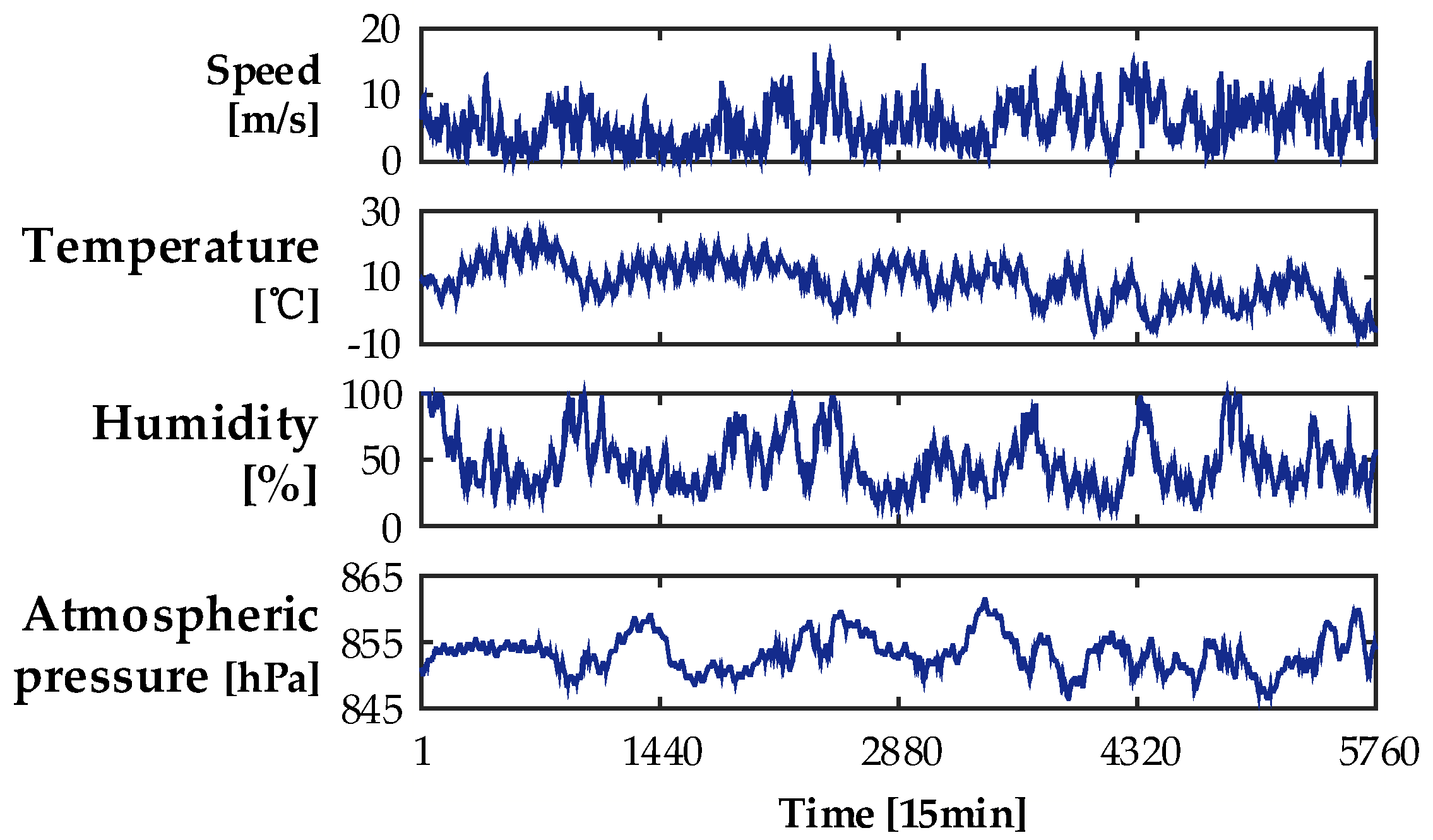
3.1. Candidate Input Variable Selection

Wind speed is significantly affected by weather factors. Therefore, temperature, humidity, and atmospheric pressure are selected as the candidate input variables. In addition, because there is a strong autocorrelation between historical and forecasted wind speeds, historical wind speed is also selected as a candidate input variable. Therefore, temperature, humidity, atmospheric pressure and historical wind speed are selected as the model input variables. The functional relationship between the original input and the output when forecasting the wind speed at any time is:

$$\mathit{y}=\mathit{f}(\mathit{spee}{\mathit{d}}^{-}, \mathit{T}\mathit{e}\mathit{m}, \mathit{H}\mathit{u}\mathit{m}\mathit{,} \mathit{Pre})$$

(5)

where $\mathit{spee}{\mathit{d}}^{-}$, $\mathit{Tem}$, $\mathit{Hum}$, and $\mathit{Pre}$ represent the wind speed, temperature, humidity, and atmospheric pressure at each current or previous time, respectively, and $\mathit{y}$ represents the forecast wind speed.

A KELM-based short-term wind speed forecasting model can be constructed by using the wind speed, temperature, humidity, and atmospheric pressure of the current and previous period as the input variables of the KELM and the wind speed of the next period as the output variable of the KELM.

3.2. KELM Modelling and GA Optimization

After the input variables have been selected from candidate input variables such as the historical wind speed, temperature, humidity, and atmospheric pressure using the RF method, the functional relationship between the input and the output of the model becomes

$$\mathit{y}=\mathit{f}({\mathit{x}}^{\prime })$$

(6)

where ${\mathit{x}}^{\prime }$ represents the optimal feature set obtained through input variable selection using the RF method.

After the model input variables have been determined, an input variable matrix containing $x^{\prime }$ and an output variable matrix containing $\mathit{y}$ can be generated. The input and output matrices are uniformly divided into training and validation sets. Then, a KELM-based model is constructed and trained. In addition, a GA is employed to optimize the regularization coefficient $C$ and the kernel function $\sigma$. The optimal KELM-based model obtained is used for forecasting. Finally, the wind speed forecast using each decomposed series is obtained.

3.3. Forecasting Results Evaluation

The final forecast value of the original wind speed is obtained by adding all the forecasts based on the decomposed series. $E_{\mathrm{MAPE}}$, the mean absolute error (MAE) $E_{\mathrm{MAE}}$, and the root mean squared error (RMSE) $E_{\mathrm{RMSE}}$ are used to evaluate the forecast obtained from the model. $E_{\mathrm{MAE}}$ and $E_{\mathrm{RMSE}}$ are calculated as follows:

$$E_{\mathrm{MAE}}=\frac{1}{k}{\displaystyle \sum _{i=1}^k|\widehat{\mathit{y}}(i)-\mathit{y}(i)|}$$

(7)

$$E_{\mathrm{RMSE}}=\sqrt{\frac{1}{k}{\displaystyle \sum _{i=1}^n{(\widehat{\mathit{y}}(i)-\mathit{y}(i))}^2}}$$

(8)

4. Case Study

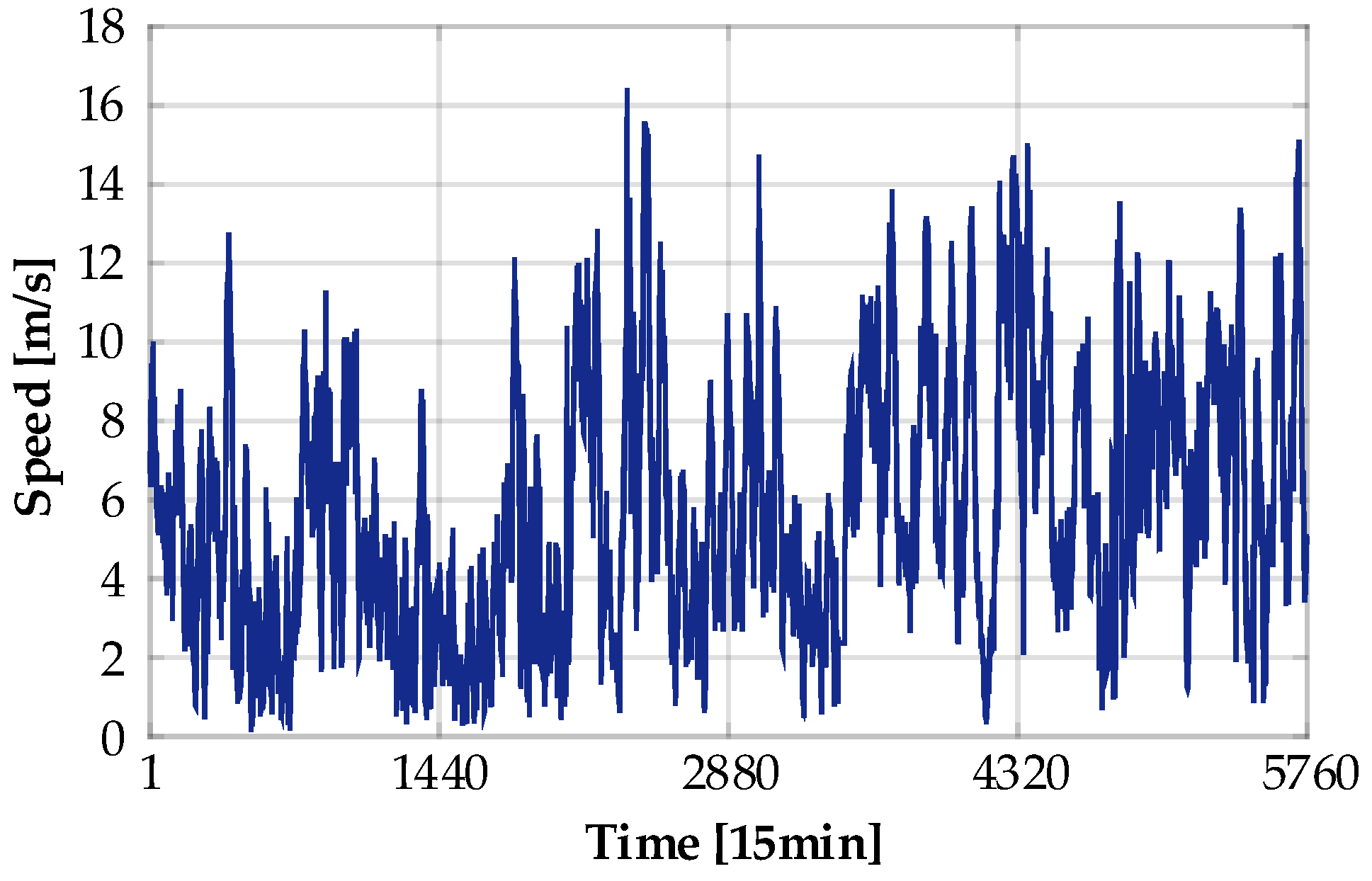
4.1. Data Source and Parameter Initialization

In this paper, a wind farm located in Hebei Province, China was used to validate the proposed method. The wind speed datasets with 15-min intervals from September to October in 2015 were collected. Figure 3 shows the wind speed with sample size of 5760, Figure 4 shows the original data of wind speed, temperature, humidity and atmospheric pressure.

In Figure 3, the maximum, minimum and average wind speeds are 16.43 m/s, 0.12 m/s and 5.76 m/s, clearly showing the large variations in wind speed. From Figure 4, it can be seen that temperature, humidity and atmospheric pressure have similar fluctuations with wind speed data sometimes and it can be inferred that they may have some relationship with wind speed. Here, 75% of the original data are used to construct the KELM-based model, and the remaining 25% are used as the test set to validate the model.

A WT is performed to decompose the original wind speed series, and the 9th-order Daubechies wavelet with three decomposition layers is adopted for WT. The original wind speed series are decomposed into one approximate series A3, and three detail series, D1, D2 and D3. Figure 5 shows the results of WT.

As shown in Figure 5, the approximation series A3 is a low-frequency signal, and very close to the original wind speed series; the detail series D1, D2 and D3 has a relatively high frequency and a relatively small amplitude, resulting in a relatively large forecasting error. So, the approximate series A3 is used to construct the forecasting model, the detail series D1, D2 and D3 are regarded as noise and neglected, and the forecast based on the approximate series A3 is used as the final result.

4.2. Candidate Input Variable Selection

In this study, the model is used to make forecasts for the next hour at time intervals of 15 min. Therefore, when selecting candidate input variables, data from the 2-h period preceding (and including) the current time are selected as the candidate input variables (i.e., the temperature, humidity, atmospheric pressure, and historical wind speed with leading periods of 1–8 × 15 min) are selected as the candidate input variables.

Table 1. Dimensions of the original input and output variables.

Variable	Matrix	Meaning	Dimension	Total Dimension
Input	$\mathit{spee}{\mathit{d}}^{-}$	$\mathit{spee}{\mathit{d}}_{t-7},\mathit{spee}{\mathit{d}}_{t-6},\dots ,\mathit{spee}{\mathit{d}}_{t-1},\mathit{spee}{\mathit{d}}_t$	8	32
	$\mathit{Tem}$	$\mathit{Te}{\mathit{m}}_{t-7},\mathit{Te}{\mathit{m}}_{t-6},\dots ,\mathit{Te}{\mathit{m}}_{t-1},\mathit{Te}{\mathit{m}}_t$	8
	$\mathit{Hum}$	$\mathit{Hu}{\mathit{m}}_{t-7}, \mathit{Hu}{\mathit{m}}_{t-6},\dots ,\mathit{Hu}{\mathit{m}}_{t-1},\mathit{Hu}{\mathit{m}}_t$	8
	$\mathit{Pre}$	$\mathit{Pr}{\mathit{e}}_{t-7},\mathit{Pr}{\mathit{e}}_{t-6},\dots ,\mathit{Pr}{\mathit{e}}_{t-1},\mathit{Pr}{\mathit{e}}_t$	8
Output	$\mathit{y}$	$\mathit{spee}{\mathit{d}}_{t+1},\mathit{spee}{\mathit{d}}_{t+2},\mathit{spee}{\mathit{d}}_{t+3},\mathit{spee}{\mathit{d}}_{t+4}$	4	4

lists the dimensions of the original input and output variables according to Equation (5).

In Table 1, $t$, $t+1$, $t+2$, $t-1$, and $t-2$ represent the current time, one lagging period (the time 15 min after the current time), two lagging periods (the time 30 min after the current time), one leading period (the time 15 min before the current time), and two leading periods (the time 30 min before the current time), respectively. As shown in Table 1, the total dimension of the candidate input variable matrices is 32, and the dimension of the original output variable matrix is 4. Because of the high dimension of the candidate input variable matrices, using all these candidate input variables directly as model inputs inevitably leads to a long training time and a poor learning result.

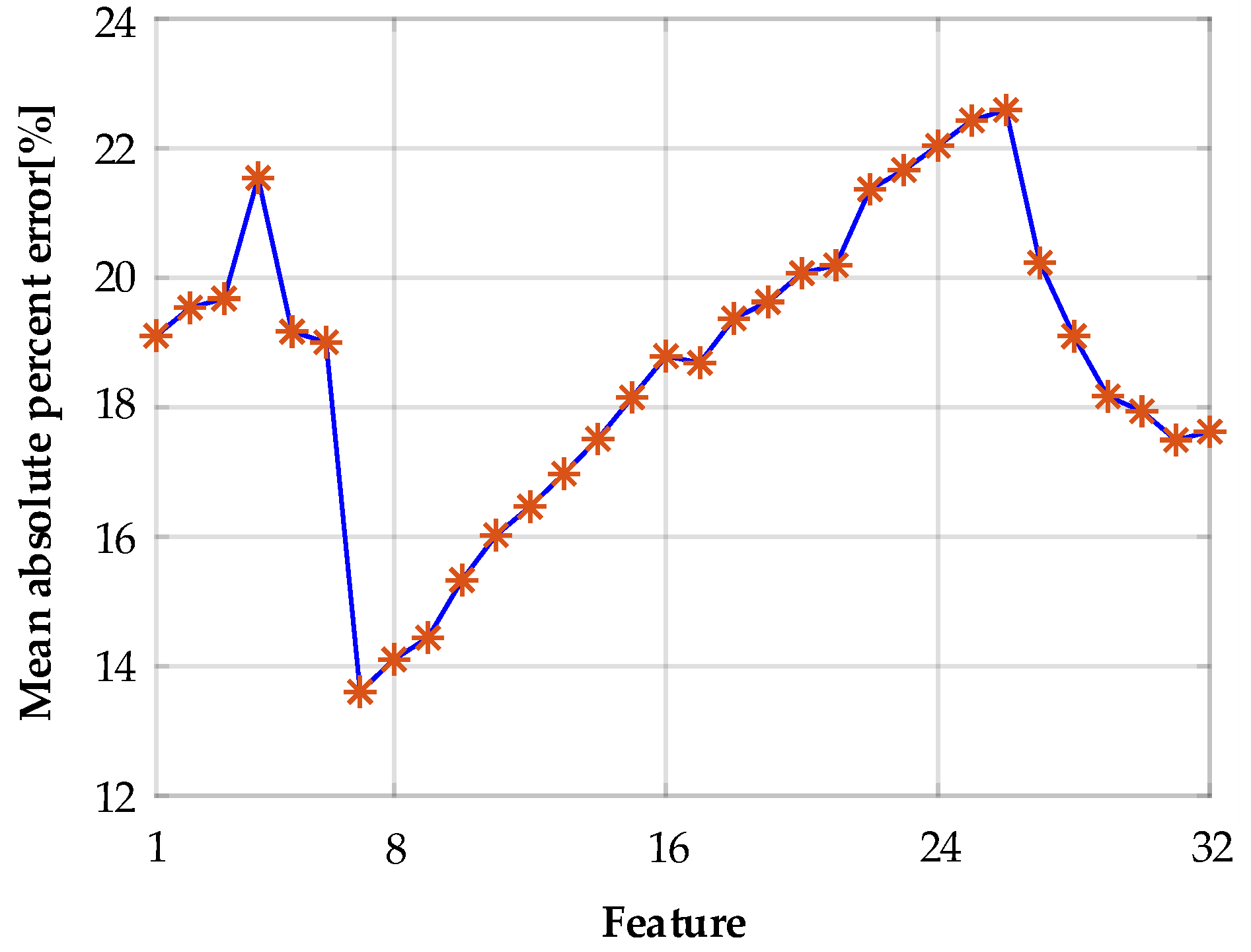
4.3. Feature Selection Based on the RF Method

The RF method is used to select a subset of features (i.e., input variables) for the model, i.e., the correlation between each feature (the wind speed $\mathit{spee}{\mathit{d}}^{-}$, the temperature $\mathit{Tem}$, the humidity $\mathit{Hum}$, and the atmospheric pressure $\mathit{Pre}$), and the forecast wind speed $\mathit{y}$ is determined by calculating $\overline{\mathit{MDA}}$ based primarily on Equation (3). Because the forecast target is the wind speed for the next 1 h period ($\mathit{spee}{\mathit{d}}_{t+1},\mathit{spee}{\mathit{d}}_{t+2},\mathit{spee}{\mathit{d}}_{t+3},\mathit{spee}{\mathit{d}}_{t+4}$), $\mathit{spee}{\mathit{d}}_{t+4}$ is used as a modelling example. The correlation between each independent variable (the historical wind speed $\mathit{spee}{\mathit{d}}^{-}$, the temperature $\mathit{Tem}$, the humidity $\mathit{Hum}$, and the atmospheric pressure $\mathit{Pre}$) and $\mathit{spee}{\mathit{d}}_{t+4}$ is calculated. Figure 6 and Figure 7 show the results for $\overline{\mathit{MDA}}$.

As shown in Figure 6, the historical wind speeds for the periods 4–11 × 15 min before the current period are highly positively correlated with $\mathit{spee}{\mathit{d}}_{t+4}$, while the correlations between them gradually decrease as the interval between the period corresponding to the historical wind speed and the current period increases. The historical wind speeds $\mathit{spee}{\mathit{d}}_t,\mathit{spee}{\mathit{d}}_{t-1}$ with periods of 4 and 5 × 15 min, respectively, are the most strongly correlated with $\mathit{spee}{\mathit{d}}_{t+4}$. As shown in Figure 7, the correlations between the temperature, humidity, and atmospheric pressure of the leading periods 4–11 × 15 min and $\mathit{spee}{\mathit{d}}_{t+4}$ are more complex. The humidity and $\mathit{spee}{\mathit{d}}_{t+4}$ correlation decreases as the leading period increases. In contrast, there is a “U”-shaped correlation between the historical temperature, the atmospheric pressure and $\mathit{spee}{\mathit{d}}_{t+4}$. The correlation between each of $\mathit{Hu}{\mathit{m}}_t,\mathit{Hu}{\mathit{m}}_{t-1}$ (the historical humidity data with leading periods of 4 and 5 × 15 min, respectively), $\mathit{Pr}{\mathit{e}}_t,\mathit{Pr}{\mathit{e}}_{t-1},\mathit{Pr}{\mathit{e}}_{t-7}$ (the historical atmospheric pressure data with leading periods of 4, 5, and 11 × 15 min, respectively) and $\mathit{spee}{\mathit{d}}_{t+4}$ is relatively significant, whereas the correlations between temperature and $\mathit{spee}{\mathit{d}}_{t+4}$ are insignificant.

Prior to the removal of feature dimensions, the optimal $E_{\mathrm{MAPE}}$ corresponding to all the candidate input variables was 17.62%. The calculation was performed in accordance with the flowchart shown in Figure 1. Each candidate input vector underwent 31 iterations. In each iteration, the feature corresponding to the smallest $\overline{\mathit{MDA}}$ was removed. Figure 8 shows the optimal $E_{\mathrm{MAPE}}$ corresponding to each iteration.

In Figure 8, the feature dimension corresponding to the smallest $\overline{\mathit{MDA}}$ is removed in each iteration. As shown in Figure 8, in each iteration, overall, $E_{\mathrm{MAPE}}$ first increases, then decreases and then increases again as features are continually removed. The initial increase in $E_{\mathrm{MAPE}}$ is a result of the decrease in the dimensionality of the data. Following the initial increase, $E_{\mathrm{MAPE}}$ continues to decrease over a long period. This decrease mainly occurs because the removal of uncorrelated and redundant features improves the model’s forecasting performance. After reaching its minimum value of 13.61%, $E_{\mathrm{MAPE}}$ begins increasing again, which occurs because the removal of useful features reduces the model’s forecasting performance.

$\mathit{B}\mathit{e}\mathit{s}\mathit{t}\_\mathit{r}\mathit{f}\mathit{S}\mathit{e}\mathit{t} = [\mathit{spee}{\mathit{d}}_{t-1},\mathit{spee}{\mathit{d}}_t, \mathit{Hu}{\mathit{m}}_{t-1},\mathit{Hu}{\mathit{m}}_t, \mathit{Pr}{\mathit{e}}_{t-7},\mathit{Pr}{\mathit{e}}_{t-1},\mathit{Pr}{\mathit{e}}_t]$ is the optimal feature subset corresponding to the smallest value of $E_{\mathrm{MAPE}}$ throughout the iteration process. This feature subset includes $\mathit{spee}{\mathit{d}}_t,\mathit{spee}{\mathit{d}}_{t-1}$ (historical wind speed data for the leading periods of 4 and 5 × 15 min, respectively), $\mathit{Hu}{\mathit{m}}_t,\mathit{Hu}{\mathit{m}}_{t-1}$ (humidity data for the leading periods of 4 and 5 × 15 min, respectively) and $\mathit{Pr}{\mathit{e}}_t,\mathit{Pr}{\mathit{e}}_{t-1},\mathit{Pr}{\mathit{e}}_{t-7}$ (atmospheric pressure data for the leading periods of 4, 5 and 11 × 15 min, respectively).

4.4. KELM-Based Modelling and Parameter Optimization

According to Equation (6), ${\mathit{x}}^{\prime }=\mathit{B}\mathit{e}\mathit{s}\mathit{t}\mathit{\_}\mathit{r}\mathit{f}\mathit{S}\mathit{e}\mathit{t} = [\mathit{spee}{\mathit{d}}_{t-1},\mathit{spee}{\mathit{d}}_t, \mathit{Hu}{\mathit{m}}_{t-1},\mathit{Hu}{\mathit{m}}_t, \mathit{Pr}{\mathit{e}}_{t-7},\mathit{Pr}{\mathit{e}}_{t-1},\mathit{Pr}{\mathit{e}}_t]$ is the optimal input variable set.

Table 2. Dimensions of the input and output variables after the selection of the input variables.

Variable	Matrix	Meaning	Dimension	Total Dimension
Input	$\mathit{spee}{\mathit{d}}^{-}$	$\mathit{spee}{\mathit{d}}_{t-1},\mathit{spee}{\mathit{d}}_t$	2	7
	$\mathit{Tem}$	-	0
	$\mathit{Hum}$	$\mathit{Hu}{\mathit{m}}_{t-1},\mathit{Hu}{\mathit{m}}_t$	2
	$\mathit{Pre}$	$\mathit{Pr}{\mathit{e}}_{t-7},\mathit{Pr}{\mathit{e}}_{t-1},\mathit{Pr}{\mathit{e}}_t$	3
Output	$\mathit{y}$	$\mathit{spee}{\mathit{d}}_{t+1},\mathit{spee}{\mathit{d}}_{t+2},\mathit{spee}{\mathit{d}}_{t+3},\mathit{spee}{\mathit{d}}_{t+4}$	4	4

lists the numbers of input and output variables of KELM.

As shown in Table 2, after processing the candidate input variables using the RF method, the dimension decreases from 32 to 7; most of the data (historical wind speed, humidity, and atmospheric pressure) have been removed. In addition, because the temperature dimension feature is insufficiently representative and redundant, it is completely removed.

Based on the selected input shown in Table 2, the KELM is trained and validated. Moreover, a GA is employed to optimize the kernel function of the KELM. After optimization, the values of $C$ and $\sigma$ are 382.5611 and 33.2767, respectively.

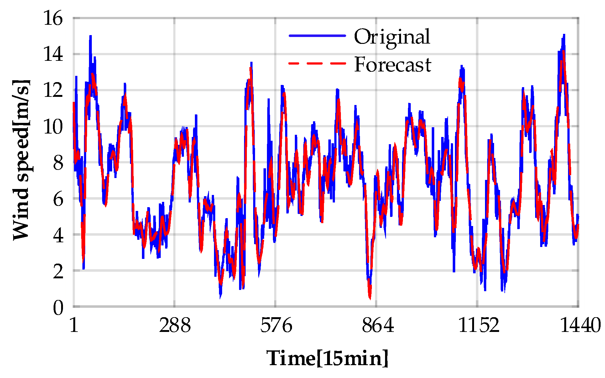
4.5. Forecasting Results and Model Comparisons

An optimal KELM-based model is obtained after GA optimization. The optimal KELM-based model is used to forecast based on the test set. Thus, forecasted wind speeds are obtained. Figure 9 shows the results.

As shown in Figure 9, the forecast values closely match the original values, which demonstrates that the model has relatively high forecasting accuracy. To examine the effectiveness of the RF method for selecting input variables, the WT-RF-KELM-GA model is compared with persistence model, RBF, NN (a feed-forward back propagation network), SVM and ELM.

Table 3. Main configuration details of each model. RBF: radial basis function; NN: neural networks; SVM: support vector machines; ELM: extreme learning machine.

Model	Configuration Details
RBF	Transfer function: Gaussian, spread of RBF: 1.
NN	Sizes of hidden layers: 5, transfer function: tansig. Parameters by GA: initial weights and thresholds.
SVM	Transfer function: Gaussian RBF. Parameters by GA: width of kernel, penalty coefficient.
ELM	Number of hidden neurons: 20, transfer function: sigmoidal. Parameters by GA: weights of input layer, bias of hidden layer.

lists the main configuration details of each model,

Table 4. Comparison of the evaluation indices of the models. MAE: mean absolute error; RMSE: root mean squared error; WT: wavelet transform.

Model	MAE (m/s)	MAPE (%)	RMSE (m/s)
Persistence	1.1782	21.83	1.1693
WT-RBF	1.3169	22.05	1.7152
WT-RF-RBF	1.0568	19.76	1.3803
WT-NN-GA	1.4018	23.36	1.6628
WT-RF-NN-GA	0.7373	13.80	0.9776
WT-SVM-GA	1.1319	21.09	1.5676
WT-RF-SVM-GA	0.7598	13.55	1.0289
WT-ELM-GA	1.2156	21.98	1.5857
WT-RF-ELM-GA	0.7688	13.83	1.0350
WT-KELM-GA	1.1694	21.54	1.5303
WT-RF-KELM-GA	0.7047	12.54	0.9518

lists the relevant evaluation indices for each model.

As shown in Table 4, after selecting the input variables using the RF method, the forecasting performance of each model increases significantly, which indicates the effectiveness of the input variables selected by the RF method. A comparison of the WT-RF-KELM-GA and WT-KELM-GA models shows that after selecting the input variables using the RF method, each evaluation index decreases by approximately 40% ($E_{\mathrm{MAE}}$: 39.7%; $E_{\mathrm{MAPE}}$: 41.8%; $E_{\mathrm{RMSE}}$: 37.8%). A comparison of the ELM, SVM, NN and RBF-based models shows that after input variable selection using the RF method, the forecasting accuracy of each model increases substantially. Therefore, the RF method effectively improves the forecasting ability of ML-based models such as the KELM, ELM, SVM, NN and RBF-based models tested here by selecting the optimal input variables. The results show the effectiveness of the input variables selected using the RF method.

5. Conclusions

This study proposed an RF-based input variable selection method that selects the optimal set of input variables to improve the forecasting accuracy of short-term wind speed forecasting models. By removing the uncorrelated and redundant features, the RF method extracts the most strongly correlated feature set from different candidate input variables for varying-length periods preceding the current period, decreases the dimensionality of the input variables, and uses the fewest features to represent the original information. It also simplifies the structure of the wind speed forecasting model and reduces its training time. The results of a case study and a comparison of several models show that the short-term wind speed forecasting model using the input variables selected by the RF method has a high learning rate, better forecasting accuracy and a higher generalization ability than other models while also requiring fewer computational resources.

The following conclusions can be drawn from this study: (1) The RF method ranks the importance of candidate input variables and then removes some of them. Extracting the most correlated features ensures that the input variables used for model input are effective, thus improving the accuracy of the wind speed forecasting model; (2) Using the RF method to select input variables for ML algorithms can effectively address the sensitivity of ML algorithms to input variables and improve the forecasting accuracy and generalization ability of ML algorithms.

References

1. Kavasseri, R.G.; Seetharaman, K. Day-ahead wind speed forecasting using f-arima models. Renew. Energy 2009, 34, 1388–1393. [Google Scholar] [CrossRef]
2. Liu, H.; Tian, H.; Li, Y. Comparison of two new ARIMA-ANN and ARIMA-Kalman hybrid methods for wind speed prediction. Appl. Energy 2012, 98, 415–424. [Google Scholar] [CrossRef]
3. Filik, T. Improved Spatio-temporal linear models for very short-term wind speed forecasting. Energies 2016, 9, 168. [Google Scholar] [CrossRef]
4. Zhang, C.; Wei, H.; Zhao, X.; Liu, T.; Zhang, K. A Gaussian process regression based hybrid approach for short-term wind speed prediction. Energy Convers. Manag. 2016, 126, 1084–1092. [Google Scholar] [CrossRef]
5. Jiang, P.; Wang, Z.; Zhang, K.; Yang, W. An innovative hybrid model based on data pre-processing and modified optimization algorithm and its application in wind speed forecasting. Energies 2017, 10, 954. [Google Scholar] [CrossRef]
6. Meng, A.; Ge, J.; Yin, H.; Chen, S. Wind speed forecasting based on wavelet packet decomposition and artificial neural networks trained by crisscross optimization algorithm. Energy Convers. Manag. 2016, 114, 75–88. [Google Scholar] [CrossRef]
7. Wang, Z.; Wang, C.; Wu, J. Wind energy potential assessment and forecasting research based on the data pre-processing technique and swarm intelligent optimization algorithms. Sustainability 2016, 8, 1191. [Google Scholar] [CrossRef]
8. Liu, D.; Niu, D.; Wang, H.; Fan, L. Short-term wind speed forecasting using wavelet transform and support vector machines optimized by genetic algorithm. Renew. Energy 2014, 62, 592–597. [Google Scholar] [CrossRef]
9. Kong, X.; Liu, X.; Shi, R.; Lee, K.Y. Wind speed prediction using reduced support vector machines with feature selection. Neurocomputing 2015, 169, 449–456. [Google Scholar] [CrossRef]
10. Santamaria-Bonfil, G.; Reyes-Ballesteros, A.; Gershenson, C. Wind speed forecasting for wind farms: A method based on support vector regression. Renew. Energy 2016, 85, 790–809. [Google Scholar] [CrossRef]
11. Huang, G.B.; Zhu, Q.Y.; Siew, C.K. Extreme learning machine: Theory and applications. Neurocomputing 2006, 70, 489–501. [Google Scholar] [CrossRef]
12. Salcedo-Sanz, S.; Pastor-Sánchez, A.; Prieto, L.; Blanco-Aguilera, A.; García-Herrera, R. Feature selection in wind speed prediction systems based on a hybrid coral reefs optimization - Extreme learning machine approach. Energy Convers. Manag. 2014, 87, 10–18. [Google Scholar] [CrossRef]
13. Zhang, C.; Zhou, J.; Li, C.; Fu, W.; Peng, T. A compound structure of elm based on feature selection and parameter optimization using hybrid backtracking search algorithm for wind speed forecasting. Energy Convers. Manag. 2017, 143, 360–376. [Google Scholar] [CrossRef]
14. Liu, D.; Wang, J.; Wang, H. Short-term wind speed forecasting based on spectral clustering and optimised echo state networks. Renew. Energy 2015, 78, 599–608. [Google Scholar] [CrossRef]
15. Huang, G.B.; Zhou, H.; Ding, X.; Zhang, R. Extreme learning machine for regression and multiclass classification. IEEE Trans. Syst. Man Cybern. Part B 2012, 42, 513. [Google Scholar] [CrossRef] [PubMed]
16. Wong, P.K.; Wong, K.I.; Chi, M.V.; Cheung, C.S. Modeling and optimization of biodiesel engine performance using kernel-based extreme learning machine and cuckoo search. Renew. Energy 2015, 74, 640–647. [Google Scholar] [CrossRef]
17. You, C.X.; Huang, J.Q.; Lu, F. Recursive reduced kernel based extreme learning machine for aero-engine fault pattern recognition. Neurocomputing 2016, 214, 1038–1045. [Google Scholar] [CrossRef]
18. Lu, F.; Jiang, C.; Huang, J.; Wang, Y.; You, C. A novel data hierarchical fusion method for gas turbine engine performance fault diagnosis. Energies 2016, 9, 828. [Google Scholar] [CrossRef]
19. Hu, M.; Hu, Z.; Yue, J.; Zhang, M.; Hu, M. A Novel Multi-Objective Optimal Approach for Wind Power Interval Prediction. Energies 2017, 10, 419. [Google Scholar] [CrossRef]
20. Lin, L.; Wang, F.; Xie, X. Random forests-based extreme learning machine ensemble for multi-regime time series prediction. Expert Syst. Appl. 2017, 83, 164–176. [Google Scholar] [CrossRef]
21. Zhang, Y.; Li, C.; Li, L. Electricity price forecasting by a hybrid model, combining wavelet transform, ARMA and kernel-based extreme learning machine methods. Appl. Energy 2017, 190, 291–305. [Google Scholar]
22. Breiman, L. Random Forests. Mach. Learn. 2001, 45, 5–32. [Google Scholar] [CrossRef]
23. Masetic, Z.; Subasi, A. Congestive heart failure detection using random forest classifier. Comput. Methods Program Biomed. 2016, 130, 54–64. [Google Scholar] [CrossRef] [PubMed]
24. Elyan, E.; Gaber, M.M. A genetic algorithm approach to optimising random forests applied to class engineered data. Inf. Sci. 2017, 384, 220–234. [Google Scholar] [CrossRef]
25. Ibrahim, I.A.; Khatib, T. A novel hybrid model for hourly global solar radiation prediction using random forests technique and firefly algorithm. Energy Convers. Manag. 2017, 138, 413–425. [Google Scholar] [CrossRef]
26. Wei, Z.S.; Han, K.; Yang, J.Y.; Shen, H.B.; Yu, D.J. Protein-protein interaction sites prediction by ensembling SVM and sample-weighted random forests. Neurocomputing 2016, 193, 201–212. [Google Scholar] [CrossRef]
Figure 1. Flowchart for random forests (RF)-based input variable selection. MAPE: mean absolute percent error; MDA: mean decrease in accuracy; kMAPE: MAPE in the current k-fold process.
Energies 10 01522 g001
Figure 2. Flowchart of the WT-RF-KELM-GA model.
Energies 10 01522 g002
Figure 3. Actual wind speed data in September and October of 2015.
Energies 10 01522 g003
Figure 4. Original data of wind speed, temperature, humidity and atmospheric pressure.
Energies 10 01522 g004
Figure 5. Original wind speed series and its decomposed series.
Energies 10 01522 g005
Figure 6. Calculated MDA values with respect to the historical wind speed. Note: Features 1–8 represent the historical wind speeds of the periods from 4–11 × 15 min before the current period, respectively.
Energies 10 01522 g006
Figure 7. Calculated MDAs with respect to the temperature, humidity, and atmospheric pressure. Notes: Features 1–8 represent the temperatures of the periods 4–11 × 15 min before the current period, respectively; features 9–16 represent the humidities of the periods 4–11 × 15 min before the current period, respectively; and features 17–24 represent the atmospheric pressures of the periods 4–11 × 15 min before the current period, respectively.
Energies 10 01522 g007
Figure 8. Relationship between prediction accuracy and number of features.
Energies 10 01522 g008
Figure 9. Wind speed forecast from the WT-RF-KELM-GA model.
Energies 10 01522 g009