Article

Lobatto-Milstein Numerical Method in Application of Uncertainty Investment of Solar Power Projects

1
Department of Mathematics, Harbin Institute of Technology, Harbin 150001, China
2
Department of Mathematics, Faculty of Science, Menoufia University, Menoufia 32511, Egypt
*
Authors to whom correspondence should be addressed.
Energies 2017, 10(1), 43; https://doi.org/10.3390/en10010043
Submission received: 5 August 2016 / Revised: 6 December 2016 / Accepted: 21 December 2016 / Published: 3 January 2017

Abstract

:
Recently, there has been a growing interest in the production of electricity from renewable energy sources (RES). The RES investment is characterized by uncertainty, which is long-term, costly and depends on feed-in tariff and support schemes. In this paper, we address the real option valuation (ROV) of a solar power plant investment. The real option framework is investigated. This framework considers the renewable certificate price and, further, the cost of delay between establishing and operating the solar power plant. The optimal time of launching the project and assessing the value of the deferred option are discussed. The new three-stage numerical methods are constructed, the Lobatto3C-Milstein (L3CM) methods. The numerical methods are integrated with the concept of Black–Scholes option pricing theory and applied in option valuation for solar energy investment with uncertainty. The numerical results of the L3CM, finite difference and Monte Carlo methods are compared to show the efficiency of our methods. Our dataset refers to the Arab Republic of Egypt.

1. Introduction

A great deal of effort is being put into researching and developing renewable energy (RE) technologies. RE can be generated from wind, solar, biomass, sunlight, tides and flowing water. The primary reason for this effort stems from the environmental impact of using fossil fuels, such as nitrogen and sulfur oxides (NOx and SOx), as well as oil spills, similar to the recent major spill in the Gulf of Mexico [1]. In addition, the rising demand for electricity is considered as one of the main reasons that also make RE development to serve to increase energy security by reducing reliability on foreign imports of fossil fuels.
Despite the delay with respect to some countries in the world, we can see the U.S., as well as several other regions, such as Western Europe, East Asia and North Africa, having a massive increase in the construction and operation of renewable power production sites. Particularly, we mean the production of electricity from renewable energy sources (RES). In the IEO2016 [2], long-term global prospects continue to improve for generating electricity from RES. RES are the fastest-growing source of energy for electricity generation, with annual increases averaging 2.9% from 2012 to 2040.
One of the RES is solar energy, which can be converted into electricity using photovoltaic (PV) technology [3,4]. Solar is the world’s fastest-growing form of RES, with net solar generation increasing by an average of 8.3%/year. Solar energy shared 859 billion kWh (15%) of the 5.9 trillion kWh of new renewable generation added over the projection period (see [5]).
The main drivers for fast-growing solar have not only been the economic efficiency and technology breakthroughs in renewable power production, but also the favorable government support due to environmental concerns. We can see that currently, such government interest in the support and incentives to private investors, but private investors are driven by profit maximization. There are two major groups of schemes that can pave the way for a wider spread: (1) the scheme of tariff-based capacity (a payment for kWh of energy generated); (2) the scheme of the quota system (the government obliges heavy industries to use a percentage of their electricity consumption from RES). Wiser et al. [6] addressed some of the government support schemes, which are typically in the form of subsidies and incentives that are front-loaded in the construction and early operating years in the U.S. Furthermore, Fagiani et al. [7] discussed the dilemma that arises from certain support schemes, such as the market risk. Regardless of the market risk factor leading to making the optimal use of RES, which implies limiting the cost to society, but the market risk simultaneously deters investors, thus this provides for less RE and a higher price.
In general, the policy instruments aim to keep investors’ risks within reasonable limits. In addition, the policies have a strong effect on the price and quantity risks faced by an investor. Therefore, we note that the drivers and investors usually feel major concern in this investment because of uncertain returns. Daim et al. [8] discussed identifying future adoption, products and technologies for residential and industrial consumers in the form of a graphical technology road map for wind energy. Sorsimo et al. [9]. presented the polices used by European nations to stimulate offshore wind development and discuss the impact of similar policies in the U.S. Furthermore, the performance of ‘market-based’ British renewable obligation and German `feed-in tariff’ systems of RE procurement systems are analyzed by Toke [10].
The RE is an uncertain investment, such that it is long term, costly and depends on a feed-in tariff system. The valuation for RE investment must consider the irreversibility and flexibility enjoyed by decision makers (i.e., the option to delay investment), in addition to the uncertainty. A.Dixit et al. [11] addressed the subject of traditional valuation techniques based on discounted cash flows inferior to real option analysis under these circumstances. Here, we follow the real option approach (ROA) to address the real option valuation (ROV) of an investment in solar energy (SE) projects and the optimal time to invest under a number of different payment settings [12,13]. Fernandes et al. [14] presented a review of the current state of the art in the application of ROA to investment in non-renewables and RES. Abadie et al. [15] provides a literature review of the real option valuation for the operation of a wind farm. According to [14,15], this particular literature in the RE sector is still limited. Therefore, attempts to fill this gap would be welcome.
In this work, we consider the ROV of private potential investment in RE under the energy and environmental policies, as well as the analysis and assessment of the impact of uncertainty sources. In other words, the ROV has a crucial dimension (the option to delay an irreversible investment in RE) under the policies and support schemes, which are provided by drivers; as such, it should be embodied in the total value of RE. A real options framework is modeled for use in RE investment using stochastic differential equation (SDEs).
Following this approach, Abadie et al. [15] addressed the value of an operating wind farm and the real option to investment in it under different support schemes. The model considers up to three sources of uncertainty: the electricity price, the wind load and the renewable obligation certificate (ROC) price. They resorted to a trinomial lattice combined with Monte Carlo simulation, when the analytical solutions are lacking. The authors considered the data referring to the U.K. Gazheli et al. [16] developed a real option model in order to take into account the uncertainty and irreversibility of the farmer deciding to lease agricultural land to a company installing a PV power plant. The uncertainty in the agricultural commodity price in addition to the irreversible science that it is a 20-year commitment from the farmer are considered. Subsidies introduced by the government to increase the investments in the RE sector are discussed. The model is applied to a province in Italy.
Stochastic differential equations (SDEs) are using to model problems in many fields of science [17]. In practice, numerical solutions are becoming increasingly important, because the analytic solutions are usually not available for SDEs. The well-known Euler–Maruyama (EM) method for SDEs was presented with a strong convergence order of 0 . 5 in [18]. In order to improve the fundamental analysis of numerical approximations, various implicit numerical methods using split-step techniques have been derived based on the Euler method. In 2002, Higham et al. [19] derived the split-step backward Euler (SSBE) method. In addition, the split-step theta (SSθ) methods, which generalize the SSBE method when θ = 1 , were discussed in [20,21]. Although, these numerical methods are A-stable for linear SDEs, these methods have a strong convergence order of 0.5. Using the additional term of the Itô–Taylor expansion, the Milstein method was presented with a strong convergence order of 1.0 [18]. Based on the Milstein method, Wang et al. [22] presented the drifting split-step backward Milstein (DSSBM) method. Guo et al. [23] constructed the modified split-step composite θ-Milstein (MSSCTM) methods. In 2015, Voss et al. [24] combined the predictor-corrector method with a Milstein method to investigate the split-step Adams–Moulton–Milstein (SSAMM) method. In 2016, the modified split-step theta Milstein (DSSθM) methods were presented by Tian et al. [25]. Although, these methods improved the convergence order to be 1.0, unfortunately, we can see that the mean-square (MS) stability conditions of these split-step methods have some restrictions for the parameters and step-size h; furthermore, these methods are not A-stable. As far as the authors know, no implicit split-step numerical methods have a strong convergence order of 1.0 and are A-stable for SDEs.
Numerical methods are needed for real option valuation in cases where analytic solutions are either unavailable or not easily comparable. Approximation of the stochastic process for an underlying asset can be applied to real option valuation. There are several candidate models for the stochastic evaluation of the underlying asset (see [26]). An overview of two numerical methods is available in the context of the Black–Scholes–Merton method [27,28]. Brennan et al. [29] considered finite difference methods (FDM). Boyle [30] gave the simulation of the stochastic process using the Monte Carlo (MC) method. The comparative study of FDM and the MC method for pricing European options was considered in [31]. In addition, the methods are typically tailored to fit into a specific problem at hand (see [32,33]).
It is well known that, when the real option can be modeled using a partial differential equation, then FDM are sometimes applied. Despite the large number of research discussed using FDM for ROV, the FDM have become uncommon in use today (particularly amongst practitioners) due to the required mathematical sophistication; these also cannot readily be used for high-dimensional problems [33]. Although the MC method has also developed, is increasing and is especially applied to high-dimensional problems, its convergence to the correct values is still slow, which leads to a significant increase in run-time [34]. Therefore, recently, there has been increasing interest in deriving new numerical methods, which can possibly avoid the shortcomings in the aforementioned methods. In this work, the new classes of split-step numerical methods are constructed, which are A-stable, with convergence with order 1.0. Using Lobatto3C (The Lobatto3C methods are algebraically stable, B-stable and L-stable. Therefore, the Lobatto3C methods are considered excellent for stiff ordinary differential equation (ODE) problems [35].) methods in collusion with the Milstein method, the Lobatto3C-Milstein (L3CM) methods are derived. The new numerical methods L3CM methods are applied to valuing the real options, and the results are compared with those of FDM and MC methods.
In this paper, a real option framework is modeled for use in RE investment. The real option framework considers the volatility in RE price during the project lifetime and the development lag between launching the project and starting the production (since the net production revenue cannot be started instantaneously, a time lag has to be allowed between the decision to establish the RE plant, and the actual production is the cost of delay (if the cash flows are evenly distributed over time and the exclusive rights last n years (20 years), the annual cost of delay can be written as: 1 n = 1 20 = 5 % a year; though, this cost of delay rises each year, to 1 19 in Year 2, 1 18 in Year 3, and so on, making the cost of delaying the exercise larger over time)). The real option framework differs from the previous work, since the new numerical methods, L3CM, are integrated with option theory and the four economic elements, cost, value, risk and flexibility, to value a real option. We examine the new L3CM methods with two other commonly-used methods, the FDM and MC methods, in an options valuation for investment with uncertainty in a case study.
The paper is organized as follows. In Section 2, we show the development in the RE sector. In addition, the investment in generating electricity using solar energy is discussed. The situation of the RE sector in Egypt is provided in Section 3. In Section 4, the L3CM methods are derived to apply in a real option framework. A real option framework is designed for use in RE investment in Section 5. In Section 6, a case study of solar thermal energy in Egypt is introduced. Furthermore, a comparison between the L3CM, FDM and MC methods is presented to explain the efficiency of the new numerical methods.

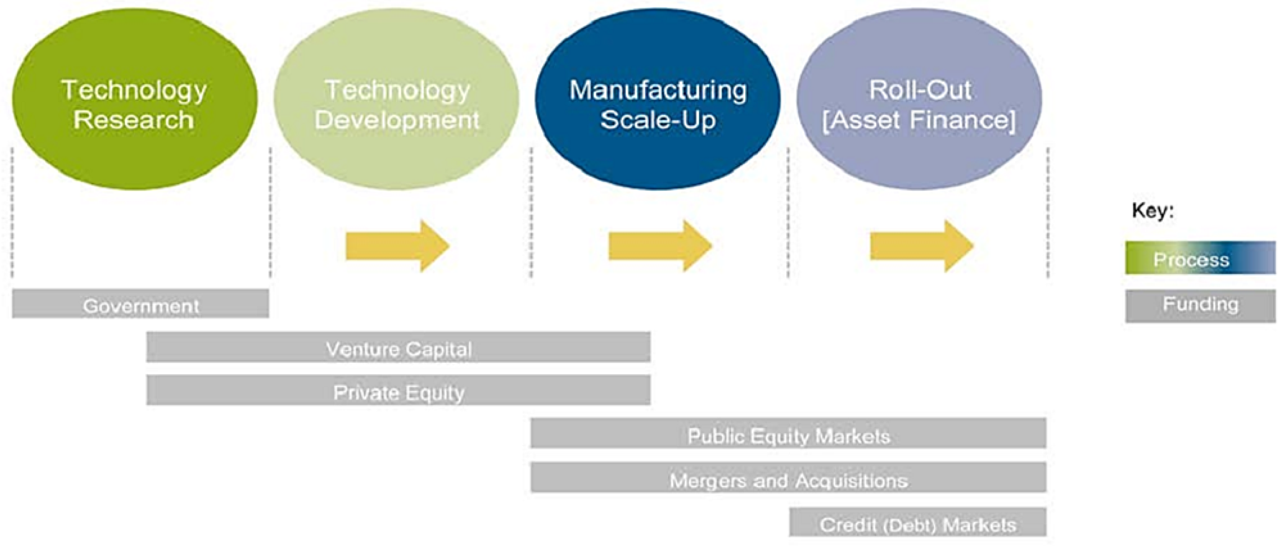
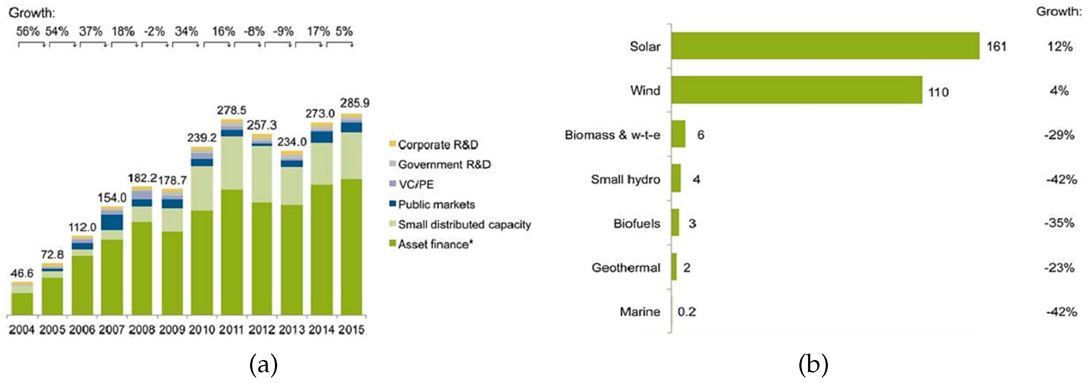
2. Renewable Energy Investment

Other concerns, like the rising demand of electricity and the risks of climate change, increase the importance of RES. In fact, RES are becoming ever more relevant in the generation of electricity. RES account for a rising share of the world’s total electricity supply, and they are the fastest growing source of electricity generation in the IEO 2016 [5] (see Figure 1). Total generation from RES increases by 2.9%/year, and the renewable share of world electricity generation grew from 22% in 2012 to 29% in 2040. The generation of electricity from solar is increasing by an average of 8.3%/year. Of the 5.9 trillion kWh of new renewable generation added over the projection period, solar energy accounts for 859 billion kWh.
A great deal of effort is being put into researching and developing renewable energy technologies. Bloomberg New Energy Finance tracks deals across the financing continuum, from R&D funding and venture capital for technology and early-stage companies, through to the asset fiance of utility-scale generation projects [36] (see Figure 2).
RE set new records in 2015. Investments reached nearly $286 billion, six-times more than in 2004. For the first time, more than half of all added power generation capacity came from RES. All of this happened in a year for which the prices of fossil fuel commodities-oil, coal and gas plummeted. So far, the drivers of investment in RE, including climate change policies and improving cost-competitiveness, have been more than sufficient to enable RE to keep growing its share of world electricity generation. Figure 3a shows that investment in RE rose 5% to $285.9 billion, taking it above the previous record of $278.5 billion reached in 2011, and that investment in RE has been running at more than $200 billion per year for six years now. The stand-out contribution to the rise in investment from the new record came from China, which lifted its outlays by 17% to $102.9 billion, some 36% of the global total. Investment also increased in the U.S., up 19% at $44.1 billion; in the Middle East and Africa, up 58% at $12.5 billion; and in India, up 22% at $10.2 billion.
Investment in solar has achieved the highest growth in 2015 among RES. Solar saw a 12% increase to $161 billion and wind a 4% boost to $109.6 billion. Biomass and waste-to-energy suffered a 42% fall to $6 billion; small hydro projects of less than 50 MW a 29% decline to $3.9 billion; biofuels a 35% drop to $3.1 billion; geothermal a 23% setback to $2 billion; and marine (wave and tidal) a 42% slip to just $215 million. Figure 3b shows the sector split for global investment.
In order to pave the way for a wider spread of investing in renewable energy, a number of public support schemes have been considered. These schemes can be divided into two major groups:
  • Regulatory price-based mechanisms (a payment for kWh of energy produced)
  • Regulatory quantity-based mechanisms (the government sets a desired level of RES, and “green” generators receive tradable certificates according to their production)
Fagiani et al. [7] point out that a dilemma arises here: market risk provides an incentive to make efficient use of resources, thus limiting the cost to society, but it simultaneously deters investors, thus potentially resulting in less RE and higher prices (as they include a higher risk premium). Regarding the support schemes, the literature has argued, especially in recent times, that a key driver of RE investment is keeping investors’ risks within reasonable limits. Three particular risk factors can stem from the policy instruments themselves:
  • The type of instrument (e.g., feed-in tariffs, tradable green certificates)
  • Constantly changing support schemes
  • The design details of the particular instrument
Policy characteristics strongly affect the price risk and the quantity risk faced by an investor. However, their scope in mitigating other sources of technical risk [37,38] and financial risk [39] is more limited. Uncertain returns on these investments are generally considered a major cause for concern for developers and investors alike.
It was stated earlier that, when valuing renewable energy projects, there is uncertainty stemming from the long-term, costly, dependency on a feed-in tariff system and random behavior of prices associated with the energy source itself. When considering solar as an RES, one of the sources of uncertainty is future solar power, as well as future electricity prices. When a storage system is considered, the uncertainty remains the same; although the storage system is in place to make the energy source more predictable, there is still uncertainty in how much solar power we will see at a given hour, as well as uncertainty in the price of electricity at a given hour. We can use real options in this setting to determine the optimal time of launching the project and assess the value of real options.

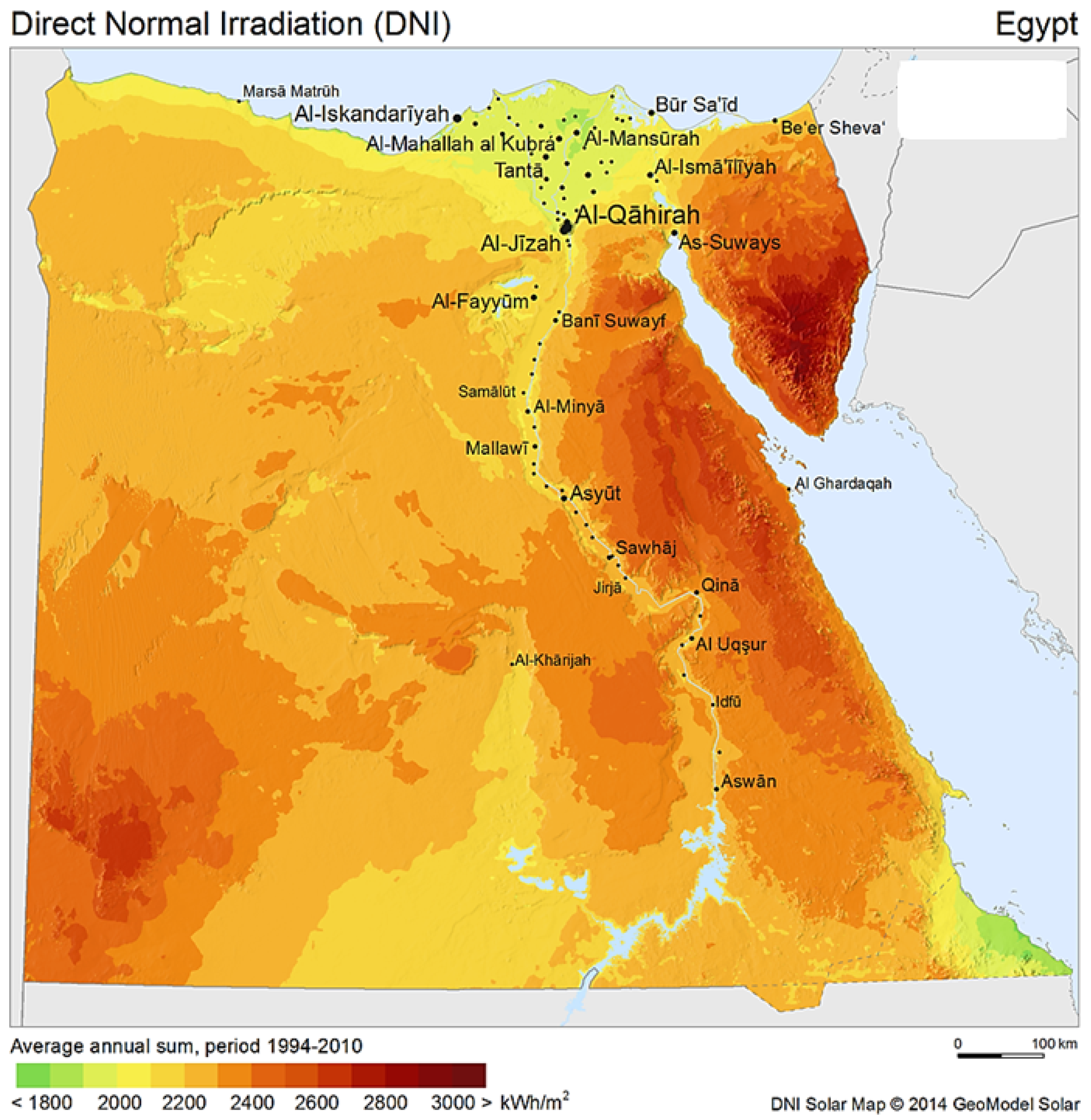
3. Renewable Energy Sector in Egypt

In this section, an overview of the RE sector in Egypt is provided. Furthermore, we show the support schemes, which are introduced by the government to increase investment opportunities in generating electricity using Solar power. In 2008, the government announced the strategic plan to reach 20% of the total electricity generated from RE by 2020 vs. 9.1% in 2013. The country enjoys a total annual global solar irradiance of up to 2.6 TWh/m 2 and a total annual sunshine duration of up to 4000 h yearly [40]. The World Bank acknowledged Egypt’s solar power advantage. It explains that there are many best areas for solar energy. Figure 4 shows the potential of solar energy in Egypt.
Fossil fuels have shared 91% of the electricity generation, in addition to 9% from RES. Of the 9% RE generation, there is 7.7% hydro-power, 1.2% wind and 0.1% solar [41]. In recent years, the Egyptian Electricity Holding Company (EEHC) has faced a gap on the power supply side, which caused recurring power cuts from 2012 to 2015. This gap will increase if the lack of investment in energy generation, both conventional and renewable, continues.
The Egyptian government has adopted an ambitious plan to reach 20% of the total electricity generated from RE by 2020, including 2% solar. The target is expected to be met by reaching the solar energy target of 3500 MW installed capacities up to 2027 [41] vs. the total capacity of 140 MW in 2014 [42]. The Egyptian government has introduced the following policies to foster the increasing of the RE energy contribution:
  • Public competitive bidding:
    Issuing tenders internationally requesting the private sector to supply power from RE projects.
  • Third party access (TPA):
    Investors are allowed to build and operate RE power plants to satisfy their electricity needs or to sell electricity to other consumers though the national grid.
  • Feed-in tariff (FIT):
    In September 2014, the government passed the key Feed-In Tariff Law (the feed-in tariff enacted by decree 1947/2014 [43,44]), triggering wide interest from international developers and investors. The main parameters of the feed-in tariffs are:
    • Solar power stations: The value of the tariff is divided into five scales according to the production capacity of the station, and the value of the tariff will be fixed during the contract period, which reaches 25 years.
    • Land allocation: Through the use of the craft scheme for a period of time equal to the contract period. Furthermore, the land will be given just 2% of the total power generated revenue from the plant. In addition, the customs will be 2% of the total items cost.
    • Electricity: That produced through renewable energy stations has priority access to the electricity grid.
    • Government support and guarantee: For power stations that exceed 500 kW, include low-interest credit facilities.
  • Net metering:
    In January 2013, EgyptERAadopted a net-metering policy that allows small-scale renewable energy projects to feed electricity to the grid. Generated surplus electricity will be discounted from the balance through the net-metering process.
  • Quota system:
    Heavy industries will be obliged to use a percentage of their electricity consumption from RE sources.
One of the challenges facing the Egyptian government to implement the RE strategy is that solar power plant investment is irreversible and uncertain. The solar energy projects are long-term, costly and depend on a feed-in tariff system. The real option framework, which takes into account investment irreversibility, uncertainty and flexibility in RE investment, was addressed in [11,16,45]. In the following, we derive new classes of numerical methods, the L3CM methods for SDEs. We discuss the applicability of the L3CM methods to approximate a stochastic process arising from real options analysis for the underlying asset in assessing the uncertainty investment.

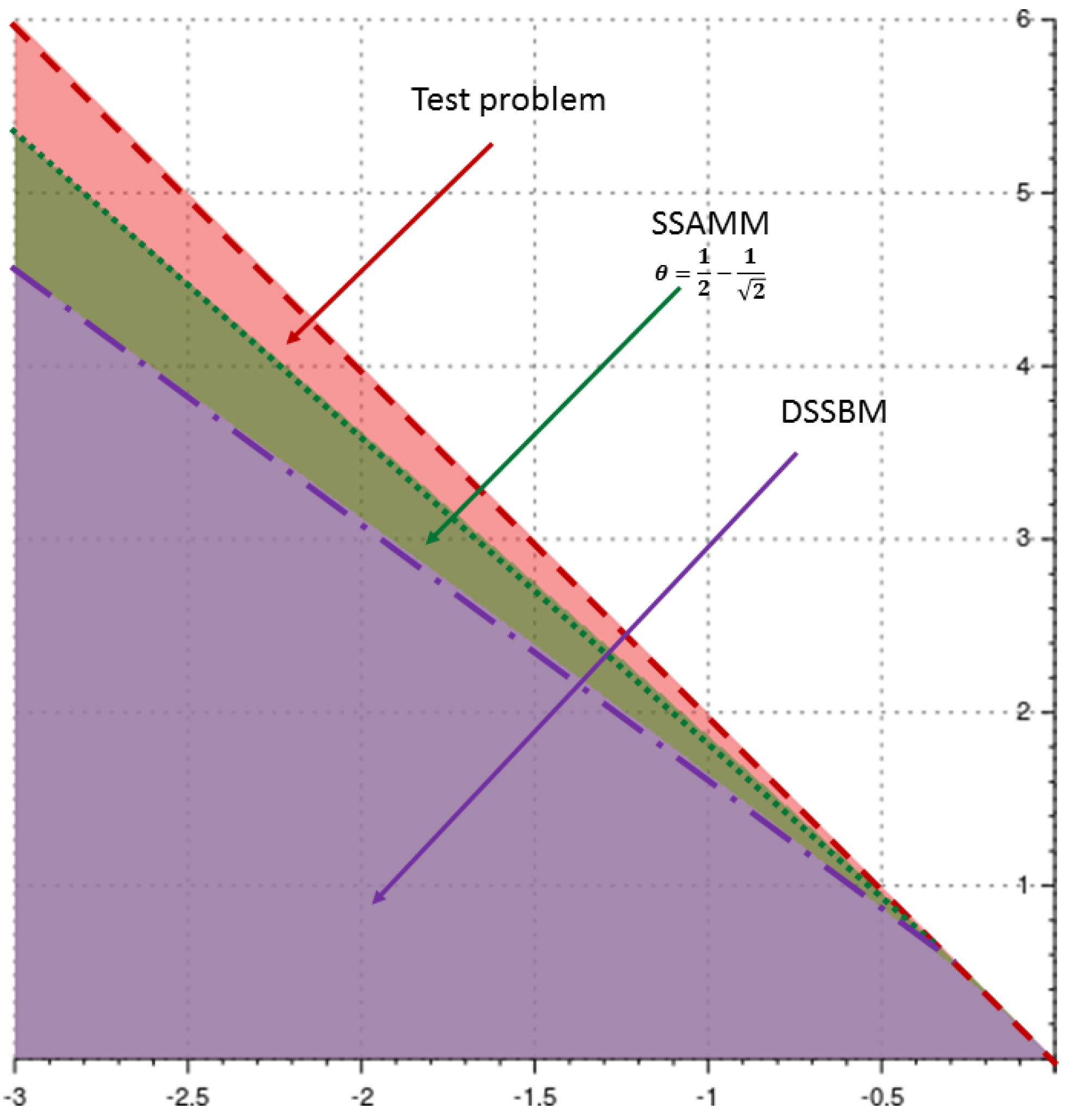
4. The Lobatto3C-Milstein Method for SDEs

Numerical methods are needed for real option valuation in cases where analytic solutions are either unavailable or not easily compatible. In this work, we construct L3CM as a new numerical method, which can be used to approximate the stochastic process for the underlying asset in real option valuation. We consider the Itô SDEs of the form:
d y ( t ) = f ( y ( t ) ) d t + g ( y ( t ) ) d W ( t ) y ( t 0 ) = y 0 t [ t 0 , T ]
where f ( y ( t ) ) is the drift coefficient, g ( y ( t ) ) is the diffusion coefficient and Wiener process W ( t ) is defined on a given probability space ( Ω , F , P ) with a filtration { F t } t 0 satisfying the usual conditions, whose increment Δ W ( t ) = W ( t + Δ t ) W ( t ) is a Gaussian random variable N ( 0 , Δ t ) .
Recently, there have been several attempts to construct numerical methods based on split-step techniques, to improve the fundamental analysis containing the convergence and stability of numerical solutions for SDEs. It is well known that there are many A-stable split-step numerical methods with a convergence order of 0.5 for scalar linear SDEs, such as the SSBE and SSθ methods. The split-step numerical methods with a convergence order of 1.0 are constructed for SDEs, for example the DSSBM method and SSAMM method. Unfortunately, we can see that the MS stability conditions of these methods for linear SDEs have some restrictions for the parameters and step-size h. Furthermore, Figure 5 shows that these methods are not A-stable.
In the following, in order to improve the numerical stability properties, the Lobatto3C-Milstein (L3CM) methods are derived for SDEs (1). The Lobatto3C note that, the Lobatto3C methods are L-stable (strong stability) and have been used successfully in solving stiff initial value ODE systems [35]) methods have the following form (the basic information about the Lobatto3C methods is presented in Appendix A):
Y n i = y n + h j = 1 s a i j f ( t n + c j h , Y n j ) i = 1 , 2 , . . . , s
y n + 1 = y n + h j = 1 s b j f ( t n + c j h , Y n j )
Now, using the Lobatto3C Formula (2) and (3) in collusion with the Milstein method, we derive the L3CM methods for SDEs (1) as follows:
Y ˜ n i = y n + h j = 1 s a i j f ( Y ˜ n j ) , i = 1 , 2 , . . . , s
y ^ n = y n + h j = 1 s b j f ( Y ˜ n j )
y n + 1 = y ^ n + g ( y ^ n ) Δ W n + 1 2 g ( y ^ n ) g ( y ^ n ) ( Δ W n ) 2 h
where y n is an approximation to X ( t n ) , s 2 is the stage value, the coefficients a i j , b j characterize the L3CM methods, with increments Δ W n : = W ( t n + 1 ) W ( t n ) being independent N ( 0 , h ) -distributed Gaussian random variables and y ( 0 ) = y 0 . Moreover, y n is { F t n } -measurable at the mesh-point t n . It is well known that the two implicit equations need to be solved for Y ˜ n i , i = 1 , . . . , s and y ^ n .
Eissa et al. [46] provided that the L3C2Mmethod (i.e., s = 2 in (4) and (5)) converges strongly with order 1.0 under the Lipschitz condition and the linear growth condition. Furthermore, the mean-square (MS) stability of the L3C2M method is investigated for SDEs with both real and complex parameters. It is shown that the L3C2M method preserves the MS-stability of the exact solutions under no restriction on the step-size in the mean-square sense. In addition, the method is A-stable. In the following, the new L3C2M method (4) to (6) will be applied in the geometric Brownian motion (GBM), which is used to model ROV (note that this geometric Brownian motion (GBM) is a special case of SDEs (1)).

5. The Real Option Framework

The valuation of real option plays an important role in the real option planning. The framework for the real option provides a special viewpoint in valuing investment with uncertainty. There are many different methods that can be applied to an ROV; these methods can be categorized into analytical and numerical methods. They can be further divided into subsections, as represented in Figure 6. Schulmerich [47] gave an overview, in-depth discussion and mathematical descriptions of some specific methods. The ROV process can be divided into five steps as follows [48]:
  • Finding uncertainty investment opportunity.
  • The probability distribution of the uncertainties is approximated.
  • Know and analyze available real options.
  • Real option valuation.
  • Develop real options mind-set: by comparing the value of the options and the cost to obtain options, a set of strategies and decisions can be reached. Meanwhile, the mind-set regarding flexibility that is available and different is established.
In this section, we consider the solar plant power as an uncertainty investment opportunity. We develop a model to assess the value of a deferred option. At any stage of the project, the model can inform a strategic option to defer the project. Based on the particular characteristics of the real option in RE investment, a deferred option of the solar power plant is considered, where the cash flows are uncertain. We assume that the revenues will start the operation time of the solar power plant (i.e., we consider the cost of delay (the time lag between the decision to establish and the actual production)).
In this real option framework, we distinguish the numerical methods of the ROV. We examine the applicability of the L3C2M method of ROV and compare the results with that of the FDM and MC methods. The L3C2M method is integrated with option theory and the four economic elements, cost, value, risk and flexibility, to value the real option. The real option framework considers the volatility in solar energy price during the project lifetime, and the development lags between launch of the project and start if the production. The decision maker is facing an uncertain utility stream for investment. The valuation of real options helps the decision maker to evaluate the investment opportunity.

5.1. Framework Application

With the solar energy investment, the solar energy is the underlying asset. The value of the asset is based on two variables, the estimation of the installed capacity (MW) of the solar energy power plant and the pricing system. To value a solar energy investment as a real option, we need to make assumptions about a number of variables as follows
  • Availability of the solar energy source:
    At the outset, since this is not known with certainty, the availability of renewables has to be estimated. The investor can estimate the installed capacity (MW) of the solar energy plant and produced energy (kWh) by environmental assessment studies.
  • Estimated cost of establishing the solar energy plant:
    The estimated development cost is the exercise price of the option. The cost of establishing the solar energy plant can be estimated by feasibility studies for the projects.
  • Time to expiration of the option:
    The life of an RE option can be defined as a contract period; that period will be the lifetime of the option. For example, the contract in the sector of RE is a long-term contract of approximately 20 to 25 years.
  • Variance in the value of the cash flows:
    The variance in the value of the cash flows is determined by two factors, variability in the pricing system of the RE and variability in the estimate of the availability of the RE. In the more realistic case where the average of the RE resources and the RE price can change over time, the option becomes more difficult to value.
  • Cost of delay:
    Since the net production revenue cannot be started instantaneously, a time lag has to be allowed between the decision to establish the solar energy plant, and the actual production is the cost of delay (If the cash flows are evenly distributed over time and the exclusive rights last n years (20 years), the annual cost of delay can be written as: 1 n = 1 20 = 5 % a year. Though, this cost of delay rises each year, to 1 19 in Year 2, 1 18 in Year 3, and so on, making the cost of delaying the exercise larger over time.).

5.2. Stochastic Model

In this model, the L3C2M numerical method is examined. GBM is used to model the ROV. Suppose that we are seeking a valuation of a project with a finite lifetime t [ 0 , T ] . The cash flows S from the investment are stochastic with a standard deviation σ and risk-free interest rate r. Hence, the evolution of cash flows over time is described as:
d S ( t ) = r S ( t ) d t + σ S ( t ) d W ( t ) t [ 0 , T ]
In the following, we derive a valuation for the investment case study problem (7) using the L3C2M numerical method. The SDEs (7) describes the paths of cash flows for the lifetime of solar power plant t [ 0 , T ] . The path values of S ( t ) can be calculated iteratively by the L3C2M method, which is introduced in the previous section. The future steps depend on the type of real option.

The Deferred Option

If we assume that a project requires an initial up-front investment of I (initial cost) and that the present value of expected cash inflows computed right at time T is S ( T ) , the value of the defer option at time T is denoted by V ( S , T ) as follows:
V ( S , T ) = e r T E [ max ( S ( T ) I , 0 ) ]
The value of the real option can be determined by calculating the expected value in (8) for a given npaths, as an approximation to the expected value. The value of S ( t ) can be determined using the L3C2M method for each path. Finally, we compare the value of real options (8) with the value of real options, which are computed by the FDM and MC method to show the efficiency of our method L3C2M.

6. A Case Study: 140-MW Solar Power Plant in Kuraymat, Egypt

In this section, we present numerical solutions for an actual case study of the solar power plant project in Egypt and analyze the numerical results. We test the evaluation model for the deferred option using the L3C2M numerical method. We demonstrate the efficiency of numerical method on the real options framework by comparing with FDM and MC methods.
Our data below are for the solar combined cycle power plant in Kuraymat, Egypt, the estimates of key parameters. They are relevant for computing revenues and initial cost over the useful lifetime. Through detailed information published in the annual report of New and Renewable Energy Authority (NREA) 2012/2013 [42], we could get and estimate the following information about the project:
  • The installed capacity is C = 140 MW, including the solar share of 20 MW (think of the total area of the integrated solar field being about 644,000 m 2 and the total solar collectors is about 1920 solar collectors containing 53,760 mirrors) (NREA annual report 2012/2013 [42]).
  • The total cost is about I = 340 $ million, and the development lag is four years (NREA annual report 2012/2013 [42]).
  • The lifetime of the project T = 25 years (the feed-in tariff enacted by decree 1947/2014 [43,44]).
  • The tariff applied to the electricity generated from solar was P = 0 . 1434 $/kWh (the feed-in tariff enacted by decree 1947/2014 [43,44]).
  • The risk-free interest rate considered is r = 8 . 75 %, which corresponds to the 10-year Egypt government debt in September 2014 (source: Egypt Central Bank [49]).
In the following, we will estimate the discount cash-flow and the variance of the purchase price of electricity from solar power plants.

6.1. Estimate Discount Cash Flows

The feed-in tariff is generally claimed to be the most effective method for promoting RE. Let P denote the fixed tariff applied to the electricity generated from the solar power plant. According to [43,44], the feed-in tariff was enacted in October 2014 and provides for a sophisticated pricing system, differentiating between solar projects, as well as project installed capacity. The keys of the pricing system are indicated; those that are relevant to international investors are:
  • 500 kW up to 20 MW: $0.136
  • 20 MW up to 50 MW: $0.1434
The capacity of the project is C = 140 MW, including the solar share of 20 MW. Therefore, the feed-in tariff is considered to be P = 0 . 1434 $/kWh. Using the total produced energy (GWh) in a given year in Table 1 [42,50], the average of producing energy (kWh/year) is estimated to be S y = 305 × 10 6 kWh/year.
The discount cash flow C F , in U.S. million dollars, of the investment under this scheme, which considers development lag, is [51]:
C F = S 0 = 0 . 1434 × 305 × 10 6 × 25 ( 1 . 9 ) 2 = 302 . 8878

6.2. Estimate the Volatility

In July 2014, the Egyptian government issued its decree 1257/2014, which determines the increase of the electricity future price gradually over five years from 2014 to 2019 [52]. This decision was made within the Egyptian government plan to reduce the energy support. In October 2014, the Egyptian government issued the feed-in tariff enacted by decree 1947/2014 [43,44], which determines the purchase price of electrical energy supplied to the Egyptian company to transport electricity, from the plants producing the electricity from RES. Furthermore, we reconsider this price after two years from the date of publication of the decree, commensurate with the change in the selling price of electricity for the user.
Using electricity selling prices stated in the decree 1257/2014 [52] and following [15], we can derive the regression model whose residuals allows us to compute the volatility:
σ = 0 . 1045
In the following Table 2, we summarized all of the data sources for the case study.

6.3. Valuation of the Deferred Option
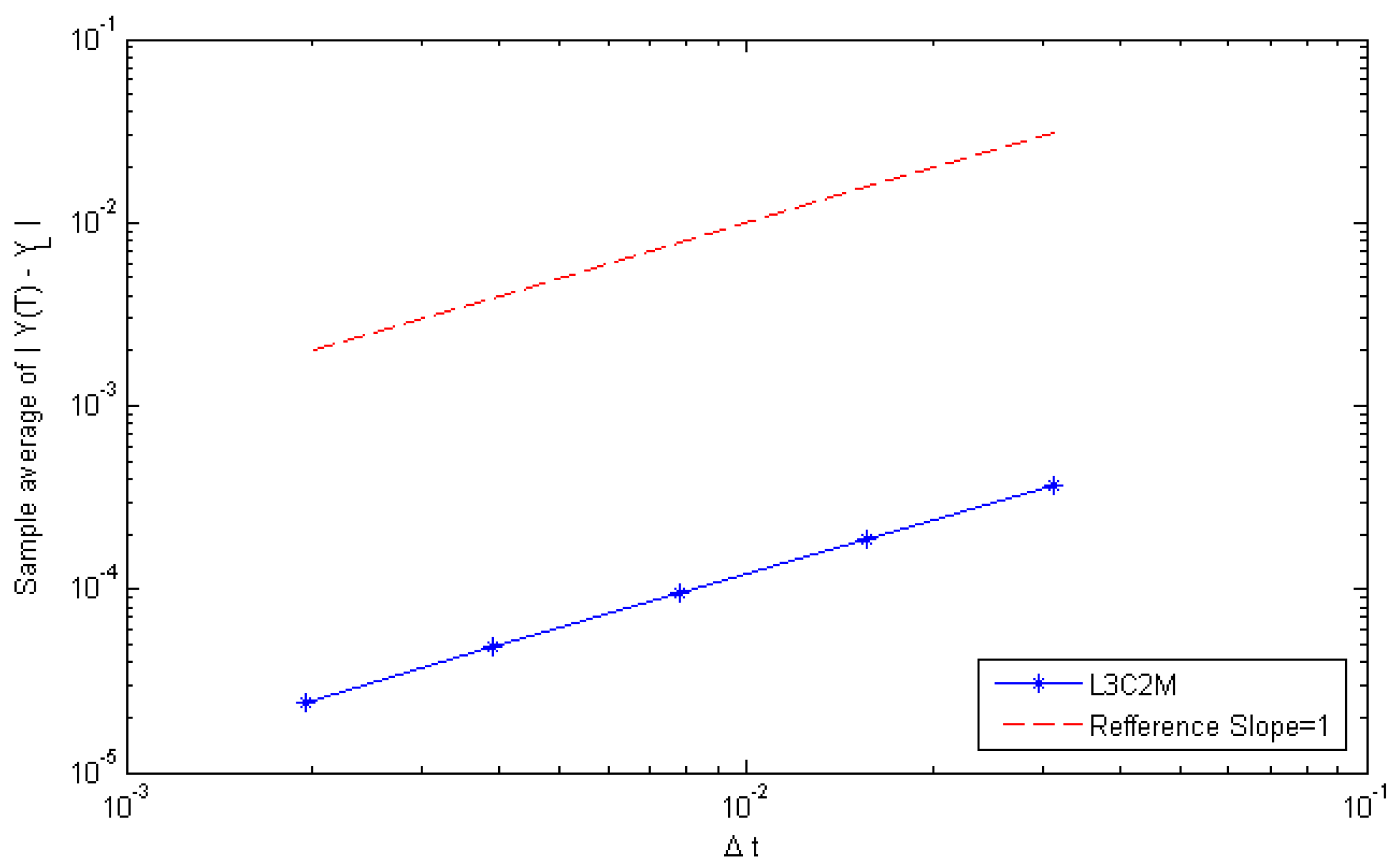
We consider the inputs in Table 2 to discuss the deferred option model as follows. We use the closed-form solution to benchmark the numerical results. A close resemblance to the pricing of a European call option (In finance, a European option can be exercised only at the expiration time of the option, while an American option can be exercised at any point of time during the option lifetime. Given the price of underlying security P and the strike price S, the payoff for a call option is defined as max ( P S , 0 ) and for a put option as max ( S P , 0 ) .) with the Black–Scholes equation [27]. Plugging the given parameters into the closed-form Black–Scholes equation yields
V e x a c t = 264 . 7410

6.3.1. L3C2M Method

We derive a numerical solution with the L3C2M method for the investment option. In addition to the parameters listed in the Table 2, we have additional parameter θ = 0 . 8 , h = 0 . 145 , such that the sample size is N = T / h , and we compute 5000 different discredited Brownian paths over the lifetime ( M = 5000 ). We get from (8):
V L 3 C 2 M = 264 . 7611
If we compare the value of the method with the exact solution, we find that the value of the method is very close to the exact solution. Moreover, note that the investment is valuated naturally in the whole domain with both methods. Comparing the option values, we note that the error in both methods is approximately the same and decreases rapidly with the length of the time steps. Figure 7 shows the mean-square error at time T versus the step-size h analyzed in the log-log diagram.

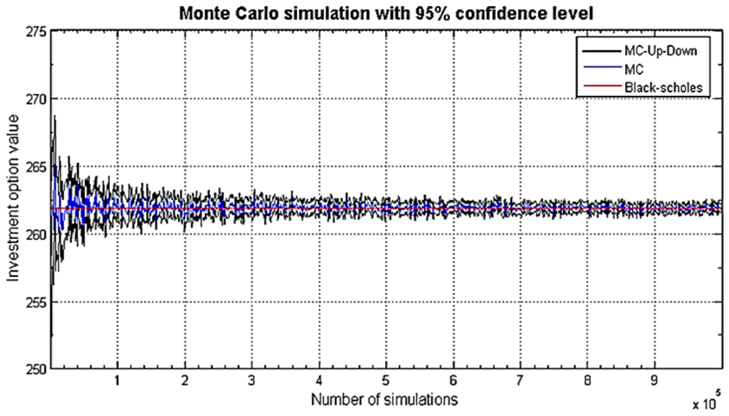
6.3.2. Monte Carlo Simulation

Following [9], we run the MC simulation with the parameters given in Table 2. Using a sample size of n m a x = 1 . 5 × 10 6 and the 95% confidence level, the simulation yields the value of the investment option:
V M C = 264 . 8050 ± 0 . 3161
We note that the value is reasonably close to the exact value. To investigate the convergence properties, we run the simulation with smaller sample sizes, descending evenly to n m i n = 5 × 10 4 . The results of the simulation are presented in Figure 8 along with the 95% confidence level.

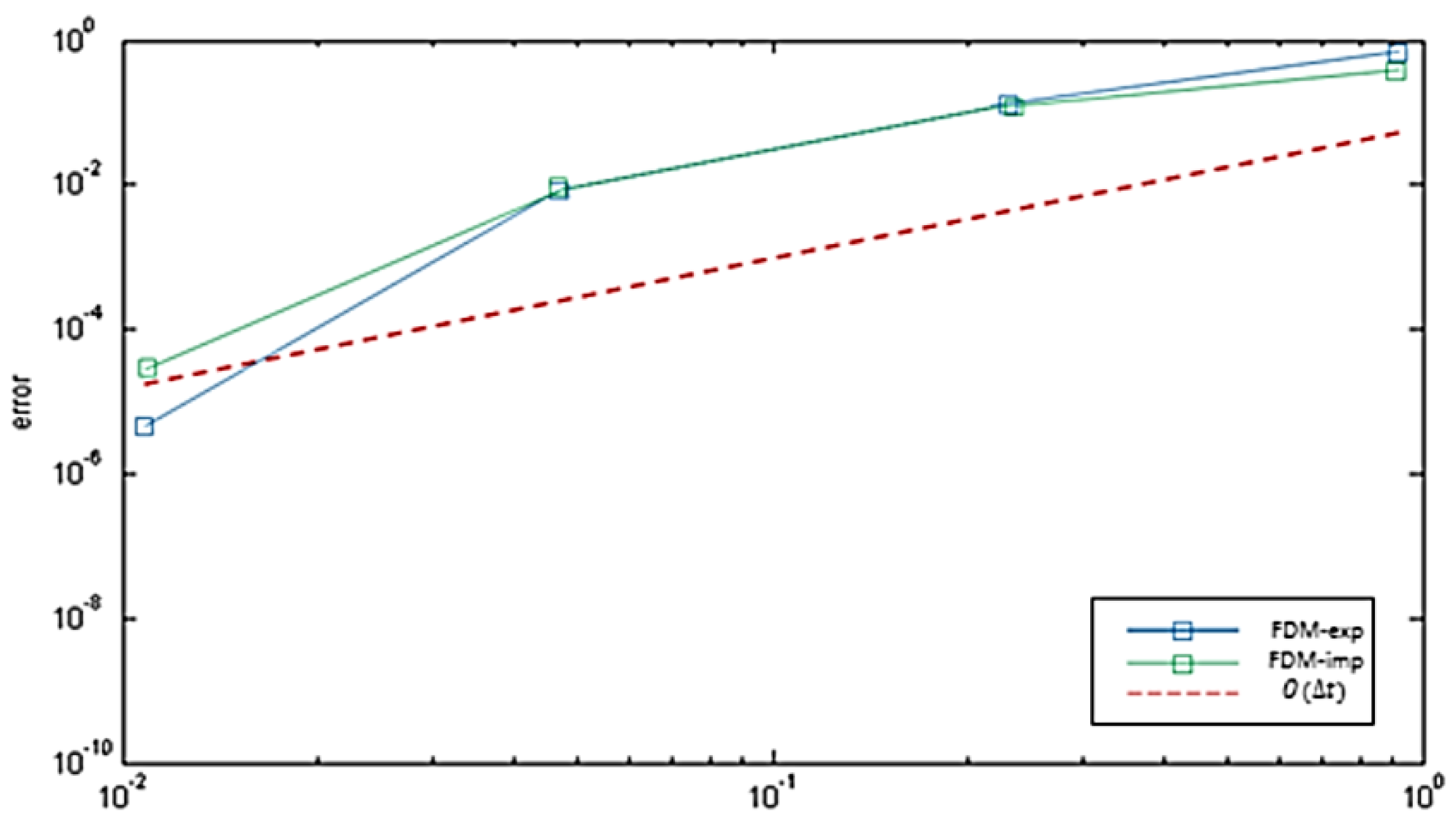
6.3.3. Finite Difference Method

Finally, following [9], we solve the investment option case with FDM. We derive a numerical solution with the explicit and implicit interpolation scheme. In addition to the parameters listed in the Table 2, we have to set additional parameters for the grid. Limiting the domain to X = 900 with N = 250 nodes and using M = 10 5 time steps, we obtain:
V F D M , e x p = 264 . 7458 V F D M , i m p = 264 . 7362
Comparing the values to the exact solution, we note that the values are very close to the exact solution with both methods. Moreover, we note that the investment is valuated naturally in the whole domain with FDM, which is not possible for example with the MC method due to path independence. The corresponding error plot of the values in log-log scale is given in Figure 9.

6.4. Discussion of the Results

Using the accuracy of the numerical solution as the only metric is problematic since increasing the number of iterations by one step does not equal increasing the grid size by one node. The comparison of the numerical methods for the investment case with respect to fixed absolute error and wall-clock time in seconds is presented in Table 3.
From Table 3, we conclude that: In general, each of the three numerical methods has values that are very close to the exact solution. Although the MC method works very well for pricing European options, approximates every arbitrary exotic option, is flexible in handling varying and even higher dimensional financial problems, the convergence of the MC method is very slow and takes a long run-time compared to other methods. FDM converges faster than the MC method and is more accurate; they are fairly robust and good for pricing options where there are the possibilities of early exercise, but FDM has become uncommonly used today, particularly amongst practitioners, due to the required mathematical sophistication; these too cannot readily be used for high-dimensional problems and also are very complicated in implementation. Finally, we can see that the L3C2M method outperforms all of the other methods in efficiency, converges faster than other methods and is considered simple in implementation compared to other methods of the case study with the given parameters.

7. Conclusions

In this paper, we address the real option valuation of an uncertainty investment in a solar power plant project and the optimal time to invest under the support program of Egypt: a feed-in tariff, electricity price and transitory subsidy. Three sources of uncertainty are considered: the electricity price, the level of solar generation and feed-in tariff. We construct a new general numerical method, the Lobatto3C-Milstein (L3CM) method, to use in the stochastic process of real option valuation, when the analytic solutions are lacking. Our real option framework differs from the previous work since; the new numerical L3CM method is integrated with option theory and the four economic elements, cost, value, risk and flexibility, to value a real option. We examine the L3CM method with two commonly-used methods, finite difference methods (FDM) and the Monte Carlo (MC) method, in an option valuation for investment with uncertainty in a case study.

Acknowledgments

The authors thanks the anonymous referees for careful reading and many helpful suggestions to improve the presentation of this paper. This research was partly financed by NSFC Grants 71350005 and 91646106. Additionally, this work is supported by the Higher Education Commission of Egypt.

Author Contributions

Mahmoud A. Eissa carried out the numerical method for SDEs, the numerical solution of the valuation problems and was relatively more involved in MATLAB. Boping Tian dealt more with the conception, theoretical issues and analysis of the results. All authors read and approved the final manuscript.

Conflicts of Interest

The authors declare that they have no competing interests.

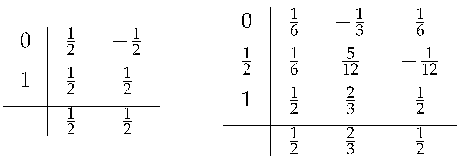
Appendix A. Background of Lobatto3C Methods

The fundamental analysis containing the convergence and stability for numerical methods for differential equations is provided in [35,53,54,55]. The families of RKmethods based on Lobatto quadrature formulas are one of several classes of fully-implicit RK methods possessing good stability properties for ODEs. The number 3 is usually found in the literature associated with Lobatto methods. Ehle [56] introduced the Lobatto 3A, 3B and 3C classes. The general definition of the Lobatto3C methods are due to [57,58]. For more information about the fundamental properties of Lobatto methods, we recommend [35,53].
The classes of s-stage Lobatto methods are given in [35]:
Y n i = y n + h j = 1 s a i j f ( t n + c j h , Y n j ) i = 1 , 2 , . . . , s
y n + 1 = y n + h j = 1 s b j f ( t n + c j h , Y n j )
where the stage value s satisfies s 2 and the coefficients a i j , b j and c j characterize the Lobatto methods. The s intermediate values Y n j for j = 1 , . . . , s are called the internal stages and can be considered as approximations to the solution at t n + c j h . The main numerical approximation at t n + 1 = t n + h is given by y n + 1 . Lobatto methods are characterized by c 1 = 0 and c s = 1 . For a fixed value of s, the various families of Lobatto methods share the same coefficients b j and c j . In addition, the coefficients a i j vary depending on the classes of Lobatto methods. For the Lobatto3C class, the a i j is defined as:
a i 1 = b 1 i = 1 , . . . , s
and determined the remaining a i j by C ( s 1 ) . The coefficients of the Lobatto3C methods can be displayed by the Butcher tableau in Figure A1.
Figure A1. The Lobatto3C methods of order two (left) and order four (right).
Energies 10 00043 g010
The stability properties of the numerical methods for deterministic ODEs are reported in [35]. In the following, we present the well-known results for Lobatto methods in a way that helps to motivate the SDEs analysis.
Proposition A1.
(See [35]) The s-stage Lobatto3C methods (A1) and (A2) applied to the scalar test equation:
d X ( t ) = λ X ( t ) d t t > 0 X ( 0 ) = X 0 0
where λ C is a constant, yields:
y n + 1 = R ( λ , h ) y n
with:
R ( Z ) = 1 + Z b T ( I Z A ) 1 1
where b T = ( b 1 , . . . , b s ) A = ( a i j ) i , j = 1 s 1 = ( 1 , . . . , 1 ) T and I is the identity matrix. R ( Z ) is called the stability function of the numerical method, which can be written for implicit methods as a rational function with numerator and denominatorof degree s as follows:
R ( Z ) = P ( Z ) Q ( Z ) d e g P = k d e g Q = j
Let S L be the stability domain for the Lobatto3C methods (A1) and (A2), then the method with stability function (A7) is A-stable if and only if | R ( i y ) | 1 for all real y, and R ( Z ) is analytic for R e Z < 0 . In addition, using the definition of the method coefficients (A3) and (Proposition 3.8 in [35]), we find that the method also is L-stable. Furthermore, the Lobatto3C methods are characterized by non-stiff order ( 2 s 2 ) , being not symmetric, algebraically stable and B-stable, and the stability function R ( z ) is given by ( s 2 , s ) Padé approximation to e z . Therefore, the the Lobatto3C methods (A1) and (A2) are described as excellent methods for stiff problems.

References

  1. World Wildlife Fund (WWF). The Energy Report—100% Renewable Energy by 2050; WWF: Gland, Switzerland, 2011. [Google Scholar]
  2. International Energy Outlook (IEO). 2016. Available online: http://www.eia.gov/forecasts/ieo/ (accessed on 5 August 2016).
  3. Andersson, B.A.; Azar, C.; Holmberg, J.; Karlsson, S. Material constraints for thin-film solar cells. Energy 1998, 23, 407–411. [Google Scholar] [CrossRef]
  4. Parida, B.; Iniyan, S.; Goic, R. A review of solar photovoltaic technologies. Renew. Sustain. Energy Rev. 2011, 15, 1625–1636. [Google Scholar] [CrossRef]
  5. EIA (2016) Updated Capital Cost Estimates for Electricity Generation Plants. Available online: www.eia.gov/forecasts/ieo/pdf/0484(2016).pdf (accessed on 5 August 2016).
  6. Wiser, R.; Bolinger, M.; Barbose, G. Using the federal production tax credit to build a durable market for wind power in the United States. Electr. J. 2007, 20, 77–88. [Google Scholar] [CrossRef]
  7. Fagiani, R.; Barquín, J.; Hakvoort, R. Risk-based assessment of the cost-efficiency and the effectivity of renewable energy support schemes: Certificate markets versus feed-in tariffs. Energy Policy 2013, 55, 648–661. [Google Scholar] [CrossRef]
  8. Daim, T.U.; Amer, M.; Brenden, R. Technology roadmapping for wind energy: Case of the Pacific Northwest. J. Clean. Prod. 2012, 20, 27–37. [Google Scholar] [CrossRef]
  9. Sorsimo, A. Numerical Methods in Real Option Analysis. Master’s Thesis, Aalto University, Helsinki, Finland, 2015. [Google Scholar]
  10. Toke, D. Renewable financial support systems and cost-effectiveness. J. Clean. Prod. 2007, 15, 280–287. [Google Scholar] [CrossRef]
  11. Dixit, A.K.; Pindyck, R.S. Investment under Uncertainty; Princeton University Press: Princeton, NJ, USA, 1994. [Google Scholar]
  12. Graham, J.R.; Harvey, C.R. The theory and practice of corporate finance: Evidence from the field. J. Financ. Econ. 2001, 60, 187–243. [Google Scholar] [CrossRef]
  13. Graham, J.; Harvey, C. How do CFOs make capital budgeting and capital structure decisions? J. Appl. Corp. Financ. 2002, 15, 8–23. [Google Scholar] [CrossRef]
  14. Fernandes, B.; Cunha, J.; Ferreira, P. The use of real options approach in energy sector investments. Renew. Sustain. Energy Rev. 2011, 15, 4491–4497. [Google Scholar] [CrossRef] [Green Version]
  15. Abadie, L.M.; Chamorro, J.M. Valuation of wind energy projects: A real options approach. Energies 2014, 7, 3218–3255. [Google Scholar] [CrossRef]
  16. Gazheli, A.; Di Corato, L. Land-use change and solar energy production: A real option approach. Agric. Financ. Rev. 2013, 73, 507–525. [Google Scholar] [CrossRef]
  17. Kloeden, P.E.; Platen, E. Numerical Solution of Stochastic Differential Equations; Springer: Berlin, Germany, 1999. [Google Scholar]
  18. Kloeden, P.E.; Platen, E. Higher-order implicit strong numerical schemes for stochastic differential equations. J. Stat. Phys. 1992, 66, 283–314. [Google Scholar] [CrossRef]
  19. Higham, D.J.; Mao, X.; Stuart, A.M. Strong convergence of Euler-type methods for nonlinear stochastic differential equations. SIAM J. Numer. Anal. 2002, 40, 1041–1063. [Google Scholar] [CrossRef]
  20. Ding, X.; Ma, Q.; Zhang, L. Convergence and stability of the split-step θ-method for stochastic differential equations. Comput. Math. Appl. 2010, 60, 1310–1321. [Google Scholar] [CrossRef]
  21. Huang, C. Exponential mean square stability of numerical methods for systems of stochastic differential equations. J. Comput. Appl. Math. 2012, 236, 4016–4026. [Google Scholar] [CrossRef]
  22. Wang, P.; Liu, Z. Split-step backward balanced Milstein methods for stiff stochastic systems. Appl. Numer. Math. 2009, 59, 1198–1213. [Google Scholar] [CrossRef]
  23. Guo, Q.; Li, H.; Zhu, Y. The improved split-step θ methods for stochastic differential equation. Math. Methods Appl. Sci. 2014, 37, 2245–2256. [Google Scholar] [CrossRef]
  24. Voss, D.A.; Khaliq, A.Q. Split-step Adams-Moulton Milstein methods for systems of stiff stochastic differential equations. Int. J. Comput. Math. 2015, 92, 995–1011. [Google Scholar] [CrossRef]
  25. Tian, B.; Eissa, M.A.; Zhang, S. Two families of theta milstein methods in a real options framework. In Proceedings of the 5th Annual International Conference on Computational Mathematics, Computational Geometry and Statistics (CMCGS 2016), Singapore, 18–19 January 2016.
  26. Copeland, T.E.; Weston, J.F.; Shastri, K. Financial Theory and Corporate Policy, 4th ed.; Pearson Addison Wesley: New York, NY, USA, 2005. [Google Scholar]
  27. Black, F.; Scholes, M. The pricing of options and corporate liabilities. J. Political Econ. 1973, 81, 637–654. [Google Scholar] [CrossRef]
  28. Merton, R.C. Theory of rational option pricing. Bell J. Econ. Manag. Sci. 1973, 4, 141–183. [Google Scholar] [CrossRef]
  29. Brennan, M.J.; Schwartz, E.S. Finite difference methods and jump processes arising in the pricing of contingent claims: A synthesis. J. Financ. Quant. Anal. 1978, 13, 461–474. [Google Scholar] [CrossRef]
  30. Boyle, P.P. Options: A monte carlo approach. J. Financ. Econ. 1977, 4, 323–338. [Google Scholar] [CrossRef]
  31. Fadugba, S.; Nwozo, C.; Babalola, T. The comparative study of finite difference method and Monte Carlo method for pricing European option. Math. Theory Model. 2012, 2, 60–66. [Google Scholar]
  32. Pringles, R.; Olsina, F.; Garcés, F. Real option valuation of power transmission investments by stochastic simulation. Energy Econ. 2015, 47, 215–226. [Google Scholar] [CrossRef]
  33. Thompson, M.; Barr, D. Cut-off grade: A real options analysis. Resour. Policy 2014, 42, 83–92. [Google Scholar] [CrossRef]
  34. Sauer, T. Numerical Analysis; Pearson: Boston, MA, USA, 2005. [Google Scholar]
  35. Hairer, E.; Wanner, G. Solving Ordinary Differential Equations II: Stiff and Differential-Algebraic Problems; Springer: Berlin, Germany, 1996. [Google Scholar]
  36. Global Trends in Renewable Energy Investment 2016, Frankfurt School UNEP Collaborating Centre for Climate and Sustainable Energy Finance. 2016. Available online: http://fs-unep-centre.org/publications/global-trends-renewable-energy-investment-2016 (accessed on 5 August 2016).
  37. Hirth, L. The market value of variable renewables: The effect of solar wind power variability on their relative price. Energy Econ. 2013, 38, 218–236. [Google Scholar] [CrossRef]
  38. Scorah, H.; Sopinka, A.; van Kooten, G.C. The economics of storage, transmission and drought: Integrating variable wind power into spatially separated electricity grids. Energy Econ. 2012, 34, 536–541. [Google Scholar] [CrossRef]
  39. Gross, R.; Blyth, W.; Heptonstall, P. Risks, revenues and investment in electricity generation: Why policy needs to look beyond costs. Energy Econ. 2010, 32, 796–804. [Google Scholar] [CrossRef]
  40. Egypt in Transition: Infrastructure and Development, British Expertise. Available online: http://www.britishexpertise.org/bx/upload/Events/Egyptintransition_Spring2015_LR.pdf (accessed on 5 August 2016).
  41. Egyptian Electricity Holding Company (EEHC). Annual Report for FY 2012/2013; EEHC: Cairo, Egypt, 2013. [Google Scholar]
  42. New and Renewable Energy Authority (NREA). Annual Report 2012/2013. Available online: http://nrea.gov.eg/annual%20report/Annual_Report_2012_2013_eng.pdf (accessed on 5 August 2016).
  43. Amereller, Investing in Renewable Energy in Egypt. January 2015. Available online: http://amereller.de/fileadmin/PDFs/ALC_Investing-in-Renewable-Energies-Jan-2015.pdf (accessed on 5 August 2016).
  44. New and Renewable Energy Authority (NREA). Available online: http://nrea.gov.eg/beta/Investors/Legislation (accessed on 5 August 2016).
  45. Min, K.J.; Lou, C.; Wang, C.H. An exit and entry study of renewable power producers: A real options approach. Eng. Econ. 2012, 57, 55–75. [Google Scholar] [CrossRef]
  46. Eissa, M.A.; Xiao, Y.; Yang, Z.Y. Lobatto3C-Milstein methods for stiff stochastic differential equations. Appl. Numer. Math. 2016. under review. [Google Scholar]
  47. Schulmerich, M. Real Options Valuation: The Importance of Interest Rate Modelling in Theory and Practice; Springer Science & Business Media: Berlin, Germany, 2010. [Google Scholar]
  48. Wang, T. Analysis of Real Options in Hydropower Construction Projects—A Case Study in China. Ph.D. Thesis, Massachusetts Institute of Technology, Cambridge, MA, USA, 2003. [Google Scholar]
  49. The Central Bank of Egypt. Available online: http://www.tradingeconomics.com/egypt/interest-rate (accessed on 5 August 2016).
  50. New and Renewable Energy Authority (NREA), Annual Report 2009/2010. Available online: http://nrea.gov.eg/annual%20report/annual2010En.pdf (accessed on 5 August 2016).
  51. Stern, N. Real Option; New York University: New York, NY, USA, 2007. [Google Scholar]
  52. Egypt’s Information Portal. Available online: http://www.eip.gov.eg/Documents/StudiesDetails.aspx?id=2142 (accessed on 5 August 2016).
  53. Hairer, E.; Nrsett, S.P.; Wanner, G. Solving Ordinary Differential Equations I: Nonstiff Problems; Springer: Berlin, Germany, 1993. [Google Scholar]
  54. Ramadan, M.; ElDanaf, T.S.; Eissa, M.A. System of ordinary differential equations solving using cellular neural networks. J. Adv. Math. Appl. 2014, 3, 182–194. [Google Scholar] [CrossRef]
  55. Ramadan, M.; ElDanaf, T.S.; Eissa, M.A. Approximate solutions of partial differential equations using cellular neural networks. Int. J. Sci. Eng. Investig. 2015, 4, 14–21. [Google Scholar]
  56. Ehle, B.L. On Pade Approximations to the Exponential Function and a-Stable Methods for the Numerical Solution of Initial Value Problems. Ph.D. Thesis, University of Waterloo, Waterloo, ON, Canada, 1969. [Google Scholar]
  57. Axelsson, O. A note on a class of strongly A-stable methods. BIT Numer. Math. 1972, 12, 1–4. [Google Scholar] [CrossRef]
  58. Chipman, F. A-stable Runge-Kutta processes. BIT Numer. Math. 1971, 11, 384–388. [Google Scholar] [CrossRef]
Figure 1. World net electricity generation from renewable power by fuel for trillion kWh [36].
Energies 10 00043 g001
Figure 2. Bloomberg New Energy Finance tracks [36].
Energies 10 00043 g002
Figure 3. Real MS-stability regions: (a) new global investment in RE by asset class; (b) new global investment in RE by sector, 2015, and growth in 2014; $BN [36].
Energies 10 00043 g003
Figure 4. Potential of solar and wind energy in Egypt (source: Solar GIS http://solargis.info).
Energies 10 00043 g004
Figure 5. Real MS-stability regions of drifting split-step backward Milstein (DSSBM), split-step Adams–Moulton–Milstein (SSAMM) and the test problem.
Energies 10 00043 g005
Figure 6. Classification of real option valuation (ROV) methods.
Energies 10 00043 g006
Figure 7. The MS error for the L3C2Mmethod.
Energies 10 00043 g007
Figure 8. The value of the investment option (blue) and the 95% confidence level with an MC simulation in comparison to the analytical solution (red).
Energies 10 00043 g008
Figure 9. Absolute error for the explicit and implicit finite difference methods (FDM).
Energies 10 00043 g009
Table 1. The total produced energy (GWh) per year.
2010/20112011/20122012/2013Average
206479230305
Table 2. Parameters used in the investment option case. NREA, New and Renewable Energy Authority.
ParameterSymbolValueUnitSource
Current CFfrom investment S 0 302.8878$US millionSection 6.1
Fixed investment costI340$US millionNREA annual report 2012/2013 [42]
Time to investT25YearsFeed-in tariff decree 1947/2014 [43,44]
S.d. of cash flowsσ0.1045 Section 6.2
Risk-free discount rater0.0875 Egypt Central Bank [49]
Table 3. Comparison of the numerical methods.
MCFDM-ExpFDM-ImpL3C2M
Inputs 100 × 10 6 (80, 9000)(80, 9000)(5000, 172)
Value (V)264.8050264.7458264.7362264.7611
Clock time48.25730.77470.60020.0695
Error V N u m . V e x a c t V e x a c t 0.000241650.000018040.000018040.0000132

