
Bioenergy from Low-Intensity Agricultural Systems: An Energy Efficiency Analysis


Abstract
:1. Introduction
2. Materials and Methods
2.1. Energy Efficiency Indicators
2.2. Comparison of the High-Intensity Industrialized and Low-Intensity Eco-Agricultural Systems
2.3. Estimating the Potential Energy Efficiency of High-Intensity Industrialized and Low-Intensity Eco-Agricultural System
2.4. Data, Conversion Factors and Assumptions
2.4.1. Data
2.4.2. Conversion Factors
2.4.3. Other Assumptions
- For alternative tractor power options
- While the energy consumed by four wheel drive > 50 HP tractors for all farm operations was obtained from detailed data provided from tractor test runs by Grisso et al. [39], for other smaller tractor implementations (two wheel drive 20–49 HP, single axle riding type 10–19 HP, ordinary single axle < 9HP), energy for ploughing was assumed to be essentially the same and/or not significantly different from those for all the other seven farm operations undertaken (assuming the required detachable implements needed to achieve the other tasks are available). This assumption was made due to lack of data for fuel consumption for all other operations (aside ploughing) by the smaller tractor implementations. As with animal labour, the assumption and resulting estimates were regarded as conservative because ploughing is the most tedious of all the farm operations. Based on the data obtained, two wheel drive 20–49 HP tractor, single axle riding type 10–19 HP tractor, ordinary single axle < 9HP tractor consume 22.5–28.0 L of diesel, 5.0–6.3 L of diesel and 16.7–25.1 L of gasoline per hectare during ploughing operations respectively. Based on the assumption, they are expected to consume approximately 180.0–224.0 L of diesel, 40.0–50.4 L of diesel, and 133.6–200.8 L of gasoline for all farm operations per hectare annually [39,55,57,58].
- For alternative tillage options
- It was assumed that there were zero energy requirements for natural, rain-fed irrigation. The zero energy consumption for rain-fed irrigation was however substituted with various amounts of energy (mostly electricity) used for powering artificial irrigation options: surface—0.2–6.5 GJ·ha−1, sprinkler—3.9–10.4 GJ·ha−1, drip—3.1–9.5 GJ·ha−1 [60,61]. Note that water is assumed to be pumped directly from surface and ground water. Energy for storage in tanks is not included.
- While the substitution of other agronomic factors was assumed not to result in significant change in maize yield, artificial irrigation was assumed to cause an increase as shown in Table 2.
- Energy for production of N, P and K fertilizers was zero if obtained from animal manure and biogas digestate. This is because they are freely delivered to the field from farm or bio-refinery plant. Only energy for transport and manure spreading was considered as fertilization costs.
- For biogas digestate, energy for lime (CaO) production and application was also zero because it is freely delivered to the field with the biogas digestate.
3. Results
4. Discussion
5. Conclusions
Supplementary Materials
Acknowledgments
Author Contributions
Conflicts of Interest
References
- Fischer, G.; Schrattenholzer, L. Global bioenergy potentials through 2050. Biomass Bioenergy 2001, 20, 151–159. [Google Scholar] [CrossRef]
- Koizumi, T. Biofuel and food security in China and Japan. Renew. Sustain. Energy Rev. 2013, 21, 102–109. [Google Scholar] [CrossRef]
- Dincer, I. Environmental impacts of energy. Energy Policy 1999, 27, 845–854. [Google Scholar] [CrossRef]
- Fischer, G.; Prieler, S.; van Velthuizen, H.; Berndes, G.; Faaij, A.; Londo, M.; de Wit, M. Biofuel production potentials in Europe: Sustainable use of cultivated land and pastures, Part II: Land use scenarios. Biomass Bioenergy 2010, 34, 173–187. [Google Scholar] [CrossRef]
- Pimentel, D. Ethanol fuels: Energy balance, economics, and environmental impacts are negative. Nat. Resour. Res. 2003, 12, 127–134. [Google Scholar] [CrossRef]
- Hill, J.; Nelson, E.; Tilman, D.; Polasky, S.; Tiffany, D. Environmental, economic, and energetic costs and benefits of biodiesel and ethanol biofuels. Proc. Natl. Acad. Sci. USA 2006, 103, 1206–11210. [Google Scholar] [CrossRef] [PubMed]
- Graham-Rowe, D. Agriculture: Beyond food versus fuel. Nature 2011, 474, S6–S8. [Google Scholar] [CrossRef] [PubMed]
- Loarie, S.R.; Lobell, D.B.; Asner, G.P.; Mu, Q.; Field, C.B. Direct impacts on local climate of sugar-cane expansion in Brazil. Nat. Clim. Chang. 2011, 1, 105–109. [Google Scholar] [CrossRef]
- Lynd, L.R.; Woods, J. Perspectives: A New Hope for Africa. Nature 2011, 474, S20–S21. [Google Scholar] [CrossRef] [PubMed]
- Grayson, M. Biofuels. Nature 2011, 474, S1–S25. [Google Scholar] [CrossRef] [PubMed]
- Savage, N. Fuels options: The ideal biofuel. Nature 2011, 474, S9–S11. [Google Scholar] [CrossRef] [PubMed]
- Altieri, M.A.; Funes-Monzote, F.R.; Petersen, P. Agroecologically efficient agricultural systems for smallholder farmers: Contributions to food sovereignty. Agron. Sustain. Dev. 2012, 32, 1–13. [Google Scholar] [CrossRef]
- Arodudu, O.T.; Helming, K.; Wiggering, H.; Voinov, A. Towards a more holistic sustainability assessment framework for agro-bioenergy systems—A review. Environ. Impact Assess. Rev. 2017, 62, 61–75. [Google Scholar] [CrossRef]
- Wiens, J.; Fargione, J.; Hill, J. Biofuels and biodiversity. Ecol. Appl. 2011, 21, 1085–1095. [Google Scholar] [CrossRef] [PubMed]
- Searchinger, T.; Heimlich, R.; Houghton, R.A.; Dong, F.; Elobeid, A.; Fabiosa, J.; Tokgoz, S.; Hayes, D.; Yu, T.H. Use of U.S. Croplands for Biofuels Increases Greenhouse Gases Through Emissions from Land-Use Change. Science 2008, 319, 1238–1240. [Google Scholar] [CrossRef] [PubMed]
- Venkat, K. Comparison of Twelve Organic and Conventional Farming Systems: A Life Cycle Greenhouse Gas Emissions Perspective. J. Sustain. Agric. 2012, 36, 620–649. [Google Scholar] [CrossRef]
- Meier, M.S.; Stoessel, F.; Jungbluth, N.; Juraske, R.; Schader, C.; Stolze, M. Environmental impacts of organic and conventional agricultural products—Are the differences captured by life cycle assessment? J. Environ. Manag. 2015, 149, 193–208. [Google Scholar] [CrossRef] [PubMed]
- Smith, M. Against ecological sovereignty: Agamben, politics and globalization. Environ. Polit. 2009, 18, 99–116. [Google Scholar] [CrossRef]
- Wezel, A.; Bellon, S.; Doré, T.; Francis, C.; Vallod, D.; David, C. Agroecology as a science, a movement and a practice. A review. Agron. Sustain. Dev. 2009, 29, 503–515. [Google Scholar] [CrossRef]
- Blesh, J.; Wolf, S.A. Transitions to agroecological farming systems in the Mississippi River Basin: Toward an integrated socioecological analysis. Agric. Hum. Values 2014, 31, 621–635. [Google Scholar] [CrossRef]
- Altieri, M.A.; Nicholls, C.I.; Henao, A.; Lana, M.A. Agroecology and the design of climate change-resilient farming systems. Agron. Sustain. Dev. 2015, 35, 869–890. [Google Scholar] [CrossRef]
- Hall, C.A.S.; Balogh, S.; Murphy, D.J.R. What is the minimum EROI that a sustainable society must have? Energies 2009, 2, 25–47. [Google Scholar] [CrossRef]
- Lambert, J.G.; Hall, C.A.S.; Balogh, S.; Gupta, A.; Arnold, M. Energy, EROI and quality of life. Energy Policy 2014, 64, 153–167. [Google Scholar] [CrossRef]
- Meyer, A.K.P.; Raju, C.S.; Kucheryavskiy, S.; Holm-Nielsen, J.B. The energetic feasibility of utilising nature conservation grasses from meadows in Danish biogas production. Resour. Conserv. Recycl. 2015, 104, 265–275. [Google Scholar] [CrossRef]
- Poisson, A.; Hall, C.A.S. Time Series EROI for Canadian Oil and Gas. Energies 2013, 6, 5940–5959. [Google Scholar] [CrossRef]
- Gagnon, N.; Hall, C.A.S.; Brinker, L. A preliminary investigation of the energy return on energy invested for global oil and gas extraction. Energies 2009, 2, 490–503. [Google Scholar] [CrossRef]
- Arodudu, O.T.; Ibrahim, E.S.; Voinov, A.; van Duren, I. Exploring bioenergy potentials of built-up areas based on NEG-EROEI indicators. Ecol. Indic. 2014, 47, 67–79. [Google Scholar] [CrossRef]
- Murphy, D.J.; Hall, C.A.S. Year in review—EROI or energy return on (energy) invested. Ann. N. Y. Acad. Sci. 2010, 1185, 102–118. [Google Scholar] [CrossRef] [PubMed]
- Voinov, A.; Arodudu, O.T.; van Duren, I.; Morales, J.; Qin, L. Estimating the potential of roadside vegetation for bioenergy production. J. Clean. Prod. 2015, 102, 213–225. [Google Scholar] [CrossRef]
- Altieri, M. Small Farms as a Planetary Ecological Asset: Five Key Reasons Why We Should Support the Revitalisation of Small Farms in the Global South. Available online: http://www.agroeco.org/doc/smallfarmes-ecolasset.pdf (accessed on 8 January 2015).
- Altieri, M.A.; Nicholls, C.I. Scaling up agroecological approaches for food sovereignty in Latin America. Development 2008, 51, 472–480. [Google Scholar] [CrossRef]
- Brander, M.; Wylie, C. The use of substitution in attributional life cycle assessment. Greenh. Gas Meas. Manag. 2011, 1, 161–166. [Google Scholar] [CrossRef]
- Weidema, B.P. Has ISO 14040/44 failed its role as a standard for LCA? J. Ind. Ecol. 2014, 18, 324–326. [Google Scholar] [CrossRef]
- IIASA. Table 38- Maximum Attainable Crop Yield Ranges (t/ha Dry Weight) for High and Intermediate level Inputs in Tropical, Subtropical and Temperate Environments under Irrigated Conditions. Available online: webarchive.iiasa.ac.at/Research/LUC/GAEZ/tab/t38.htm (accessed on 19 October 2014).
- IIASA. Table 39- Average of Year 1960–1996 Simulated Maximum Attainable Crop Yield Ranges (t/ha Dry Weight) for High, Intermediate and Low Level Inputs in Tropical, Subtropical and Temperate Environments under Rain-Fed Conditions. Available online: webarchive.iiasa.ac.at/Research/LUC/GAEZ/tab/t39.htm (accessed on 19 October 2014).
- IFA. Maize/Corn: Fertilizer Best Management Practices. Crop Nutrition Wikidot: International Fertilizer Application. Available online: www.cropnutrition.wikidot.com/maize-corn (accessed on 19 October 2014).
- Patzek, T. Thermodynamics of the corn-ethanol biofuel cycle. Crit. Rev. Plant Sci. 2004, 23, 519–567. [Google Scholar] [CrossRef]
- ORNL. Conversion Factors for Bioenergy. Oak Ridge National Laboratory, U.S. Department of Energy. Available online: https://content.ces.ncsu.edu/conversion-factors-for-bioenergy (accessed on 22 December 2016).
- Grisso, R.; Perumpral, J.V.; Vaughan, D.; Roberson, G.T.; Pitman, R. Predicting Tractor Diesel Fuel Consumption; Virginia Cooperative Extension, Virginia Tech; Virginia State University: Petersburg, VA, USA, 2010; p. 10. [Google Scholar]
- Arodudu, O.T.; Voinov, A.; van Duren, I. Assessing bioenergy potentials in rural areas. Biomass Bioenergy 2013, 58, 350–364. [Google Scholar] [CrossRef]
- Graboski, M.S. Fossil Energy Use in the Manufacture of Corn Ethanol. A Report for the National Corn Growers Association; Colorado School of Mines: Golden, CO, USA, 2002; p. 113. [Google Scholar]
- Galitsky, C.; Worrel, E.; Ruth, M. Energy Efficiency Improvement and Cost Saving Opportunities for the Corn Wet Milling Industry. An Energy Star® Guide for Energy and Plant Managers; Ernest Orlando Lawrence Berkeley National Laboratory, University of California: Berkeley, CA, USA, 2003; p. 84. [Google Scholar]
- Uellendahl, H.; Wang, G.; Møller, H.B.; Jørgensen, U.; Skiadas, I.V.; Gavala, H.N.; Ahring, B.K. Energy balance and cost-benefit analysis of biogas production from perennial energy crops pretreated by wet oxidation. Water Sci. Technol. 2008, 58, 1841–1847. [Google Scholar] [CrossRef] [PubMed]
- White, P.J.; Johnson, L.A. Corn Chemistry and Technology; American Association of Cereal Chemists: St. Paul, MN, USA, 2003; p. 892. [Google Scholar]
- Bonnardeaux, J. Potential Uses for Distillers Grains. Department of Agriculture and Food, Government of Western Australia: South Perth, Australia. Available online: https://www.agric.wa.gov.au/ (accessed on 19 October 2014).
- Naylor, R.L.; Liska, A.J.; Burke, M.B.; Falcon, W.P.; Gaskell, J.C.; Rozelle, S.D.; Cassman, K.G. The Ripple Effect: Biofuels, Food Security, and the Environment. Environment 2007, 49, 30–43. [Google Scholar] [CrossRef]
- Heney, J. Talking about Money: Explaining the Finances of Machinery Ownership; Rural Infrastructure and Agro-Industries Division, Food and Agriculture Organization of the United Nations: Rome, Italy, 2009. [Google Scholar]
- Belfield, S.; Brown, C. Field Crop Manual: Maize—A Guide to Upland Production in Cambodia; New South Wales Department of Primary Industries: Orange, Australia, 2008; p. 43. [Google Scholar]
- Food and Agriculture Organization of the United Nations (FAO). Environment and Natural Resources Working Paper No. 4; FAO: Rome, Italy, 2000. [Google Scholar]
- Joshi, D.D. Livestock Rearing; Myers, M.L., Stellman, J.M., Eds.; International Labour Organization: Geneva, Switzerland, 2011. [Google Scholar]
- Naudé-Moseley, B.; Jones, P.A. Donkeys Don’t Need Roads. Available online: https://www.researchgate.net/publication/236347326_with_B_Naude-Moseley_Donkeys_don%27t_need_roads_Farmer%27s_Weekly_92046Grow_22_November_4 (accessed on 12 October 2013).
- Christians, N.E. Preemergence Weed Control Using Corn Gluten Meal. U.S. Patent 5,030,268, 9 July 1991. [Google Scholar]
- Bomford, M.; Silvernail, A.; Peterson, A.; Detenber, S. Corn Gluten Meal as Organic Herbicide: A Worthwhile Investment for Organic Growers? Agricultural Sciences Section, Kentucky Academy of Science Meeting: Morehead, KY, USA, 2006. [Google Scholar]
- Gebrezgabher, S.A.; Meuwissen, M.P.M.; Oude Lansink, A.G.J.M.; Prins, B.A.M. Economic analysis of anaerobic digestion: A case of green power biogas plant in The Netherlands. In Proceedings of the 18th International Farm Management Congress, Bloomington, IL, USA, 19–24 July 2009; pp. 231–244.
- KWS. Biogas in Practice; KWS UK Limited: Hertfordshire, UK, 2012; p. 38. [Google Scholar]
- United Nations Asia Pacific Centre for Agricultural Engineering and Machinery (UNAPCAEM), Beijing, P.R. China. Country Report: Sri Lanka; Available online: http://unapcaem.org/activities%20files/a07/country%20paper-sri%20lanka(hanoi%2004).pdf (accessed on 6 October 2013).
- National Centre for Agricultural Mechanization (NCAM). Report of the National Centre for Agricultural Mechanization on Vari Mini Multi-Purpose Tractor; NCAM: Ilorin, Nigeria, 2011; p. 10. [Google Scholar]
- Kulkarni, M. Greaves launches mini tractor. Business Standard, 15 April 2013. [Google Scholar]
- Cropwatch. Tillage Systems Descriptions. Cropwatch, University of Nebraska-Lincoln: United States, 2013; Available online: http://cropwatch.unl.edu/tillage (accessed on 12 October 2013).
- Jacobs, S. Comparison of Life Cycle Energy Consumption of Alternative Irrigation Systems. Ph.D. Thesis, University of Southern Queensland, Toowoomba, Australia, 2006. [Google Scholar]
- Jackson, T. An Appraisal of the On-Farm Water and Energy Nexus in Irrigated Agriculture. Ph.D. Thesis, Charles Sturt University, Bathurst, Australia, 2009. [Google Scholar]
- Goldenberg, S. GM Corn Being Developed for Fuel Instead of Food; The Guardian: London, UK, 2011. [Google Scholar]
- Goho, A.M. Corn Primed for Making Biofuel. MIT Technology Review: Big Sandy, TX, USA, 2008; Available online: http://www.technologyreview.com/news/409913/corn-primed-for-making-biofuel/ (accessed on 12 October 2013).


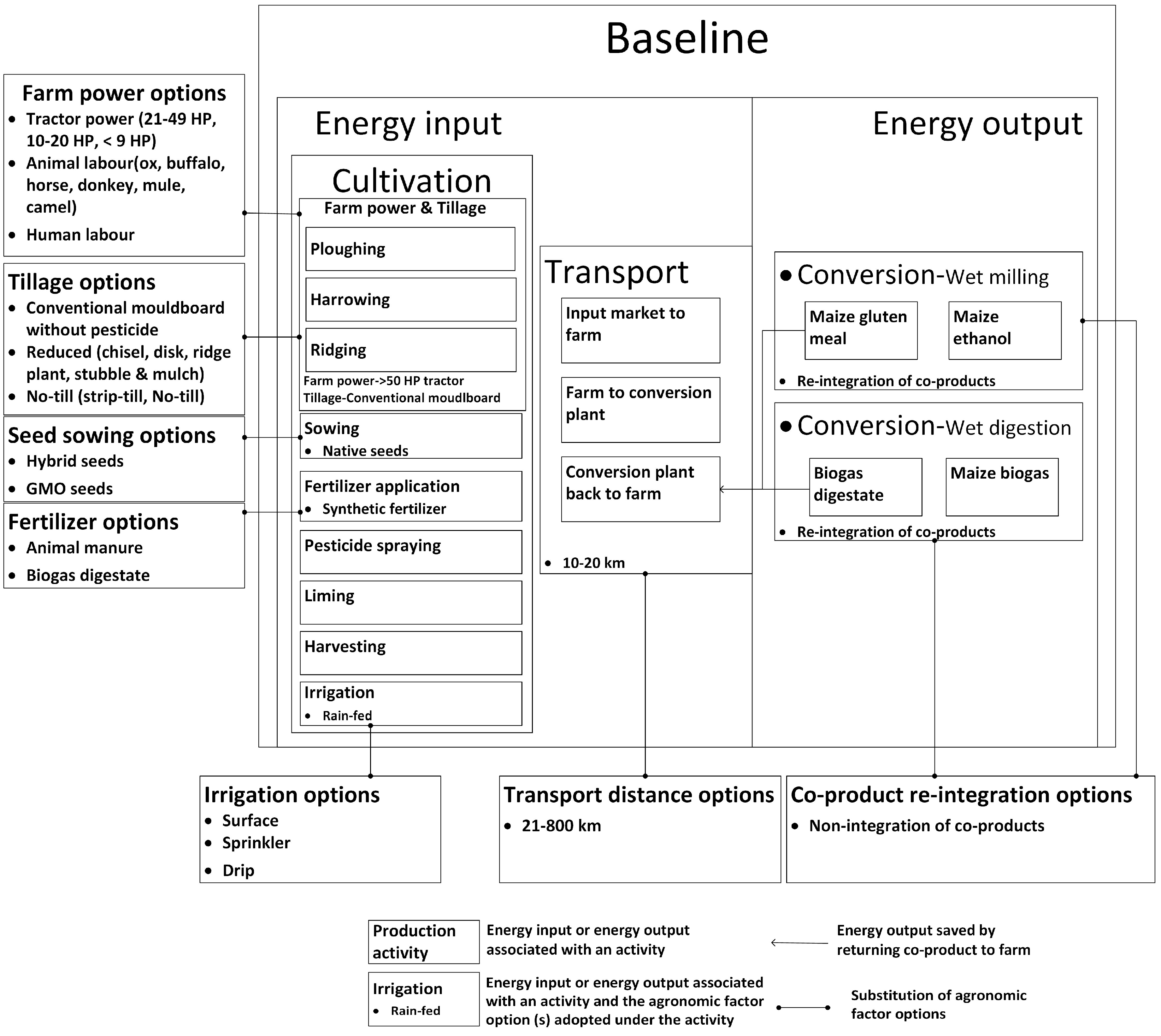
| Agronomic Factor | High-Intensity Industrialized Agriculture | Low Intensity Eco-Agricultural Systems |
|---|---|---|
| Farm power | Mostly large tractor driven (four wheel drive > 50 HP and two wheel drive 20–49 HP tractors) | Smaller tractor implementations encouraged (single axle riding type 10–19 HP and ordinary single axle < 9 HP tractors). Substitution of tractors with human and animal (mostly ox, buffalo, horse, donkey, mule and camel) labour. |
| Tillage | Conventional mouldboard tillage with and without pesticide application | Reduced tillage options (e.g., chisel, disk, ridge plant, and stubble and mulch) and no tillage options (e.g., strip-till and no-till) |
| Fertilizer | Expensive, synthetic (inorganic) fertilizers for maximum productivity and higher profit margins | Cheap, renewable (naturally available and/or organic) waste based fertilizer options such as animal manure, biogas digestates, decaying straws etc. |
| Seed-sown | Hybrid and genetically modified(GMO) seeds for maximum productivity and higher profit margins | Native seeds are encouraged |
| Irrigation | Drip and sprinkler irrigation systems for precision farming | Rain-fed and surface irrigation systems |
| Co-product reintegration | Reintegration of co-products as fertilizers and pesticides not prioritized | Reintegration of co-products as fertilizers and pesticides encouraged |
| Transport distances | 21–800 km between input market, farm and plant | 10–20 km between input market, farm and plant |
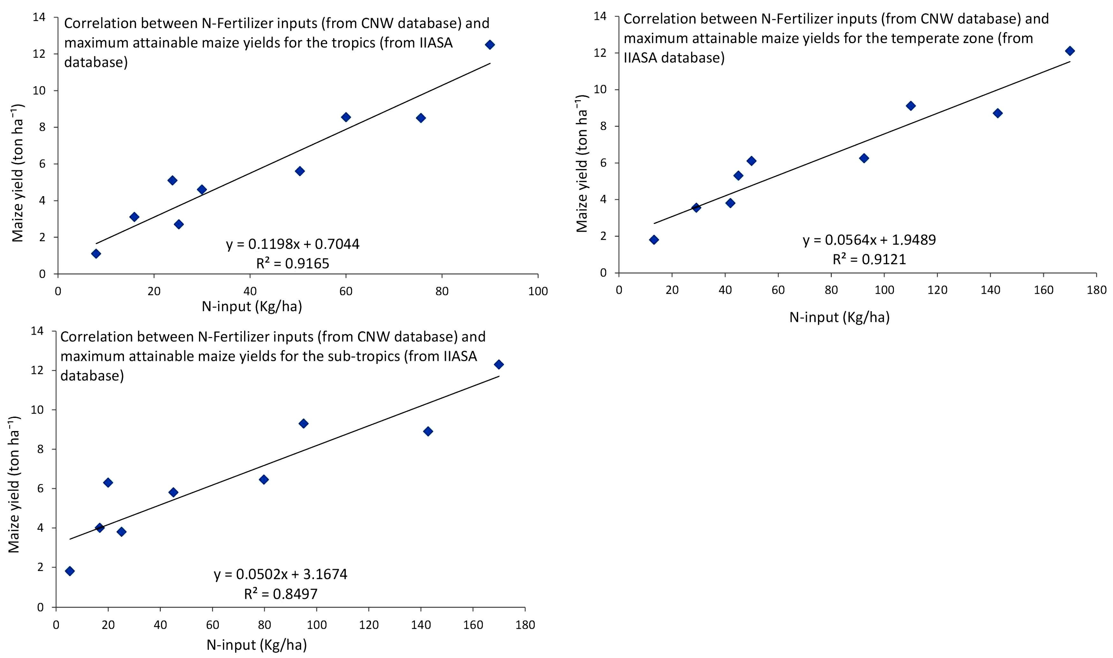
| Agro-Climatic Zones | Tropics—Brazil, Thailand, Philippines, Indonesia | Sub-Tropics—India, South Africa | Temperate—France, United States | ||||||
|---|---|---|---|---|---|---|---|---|---|
| Input Regime | Low | Intermediate | High | Low | Intermediate | High | Low | Intermediate | High |
| N-Fertilization rates (kg·ha−1) | 8.0–23.9 | 25.2–75.6 | 30.0–90.0 | 5.3–45.1 | 16.8–142.8 | 20.0–170.0 | 13.3–45.1 | 42.0–142.8 | 50.0–170.0 |
| P-Fertilization rates (kg·ha−1) | 30.0–50.0 | 45.0–80.0 | 45.0–90.0 | 45.0–60.0 | 60.0–100.0 | 100.0–300.0 | 53.0–55.0 | 56.0–62.5 | 62.5–84.0 |
| K-Fertilization rates (kg·ha−1) | 0.0–30.0 | 15.0–60.0 | 30.0–60.0 | 30.0–45.0 | 45.0–120.0 | 82.5–120.0 | 56.0–57.0 | 66.0–85.0 | 85.0–93.5 |
| Maximum attainable harvested grain yield under rain-fed irrigation (t·ha−1·a−1) | 1.1–5.1 | 2.7–8.5 | 4.6–12.5 | 1.8–5.8 | 4.0–8.9 | 6.3–12.3 | 1.8–5.3 | 3.8–8.7 | 6.1–12.1 |
| Maximum attainable harvested grain yield under artificial irrigation (t·ha−1·a−1) | - | 3.5–10.5 | 6–15.6 | - | 5.3–12.2 | 6.1–12.1 | - | 4.9–11.3 | 6.1–12.1 |
| Energy from Co-Products of Ethanol Production (Maize Gluten Meal) [37,38,52,53] | |
| Proportion of maize gluten meal per ton of maize (kg·t−1) | 36.3–57.0 |
| Energy saved by use of maize gluten meal as herbicide replacement (MJ·kg−1) | 2.1–4.7 |
| Energy saved by use of maize gluten meal as herbicide replacement (MJ·t−1) | 76.2– 267.9 |
| Energy saved by use of maize gluten meal as N-fertilizer replacement (MJ·kg−1) | 43.0–65.3 |
| Percentage of N-fertilizer in maize gluten meal (%) | 10.0 |
| Energy saved by use of maize gluten meal as N-fertilizer replacement (MJ·t−1) | 325.1–1749.4 |
| Total energy from co-products (ethanol) (MJ·t−1) | 401.3–2017.3 |
| Energy from Co-Products of Biogas Production (Biogas Digestate) [54,55] | |
| Ratio of digestate to biomass (%) | 96.0–98.0 |
| Energy for producing lime saved by use of biogas digestate (MJ·kg−1) | 0.6–1.8 |
| Energy for producing N-fertilizer saved by use of biogas digestate (MJ·kg−1) | 43.0–65.3 |
| Energy for producing P-fertilizer saved by use of biogas digestate (MJ·kg−1) | 4.8–32.0 |
| Energy for producing K-fertilizer saved by use of biogas digestate (MJ·kg−1) | 5.3–13.8 |
| Quantity of Lime in biogas digestate (kg·t−1) | 0.8 |
| Quantity of N-fertilizer in biogas digestate (kg·t−1) | 3.7–16.1 |
| Quantity of P-fertilizer in biogas digestate (kg·t−1) | 1.8–19.8 |
| Quantity of K-fertilizer in biogas digestate (kg·t−1) | 4.5–32.0 |
| Energy from co-products (Lime energy replacement) (MJ·t−1) | 0.5–1.4 |
| Energy from co-products (N-fertilizer energy replacement (MJ·t−1) | 152.7–1030.3 |
| Energy from co-products (P-fertilizer energy replacement) (MJ·t−1) | 8.3–620.9 |
| Energy from co-products (K-fertilizer energy replacement) (MJ·t−1) | 22.9–432.8 |
| Total energy from co-products (biogas) (MJ·t−1) | 184.4–2085.4 |
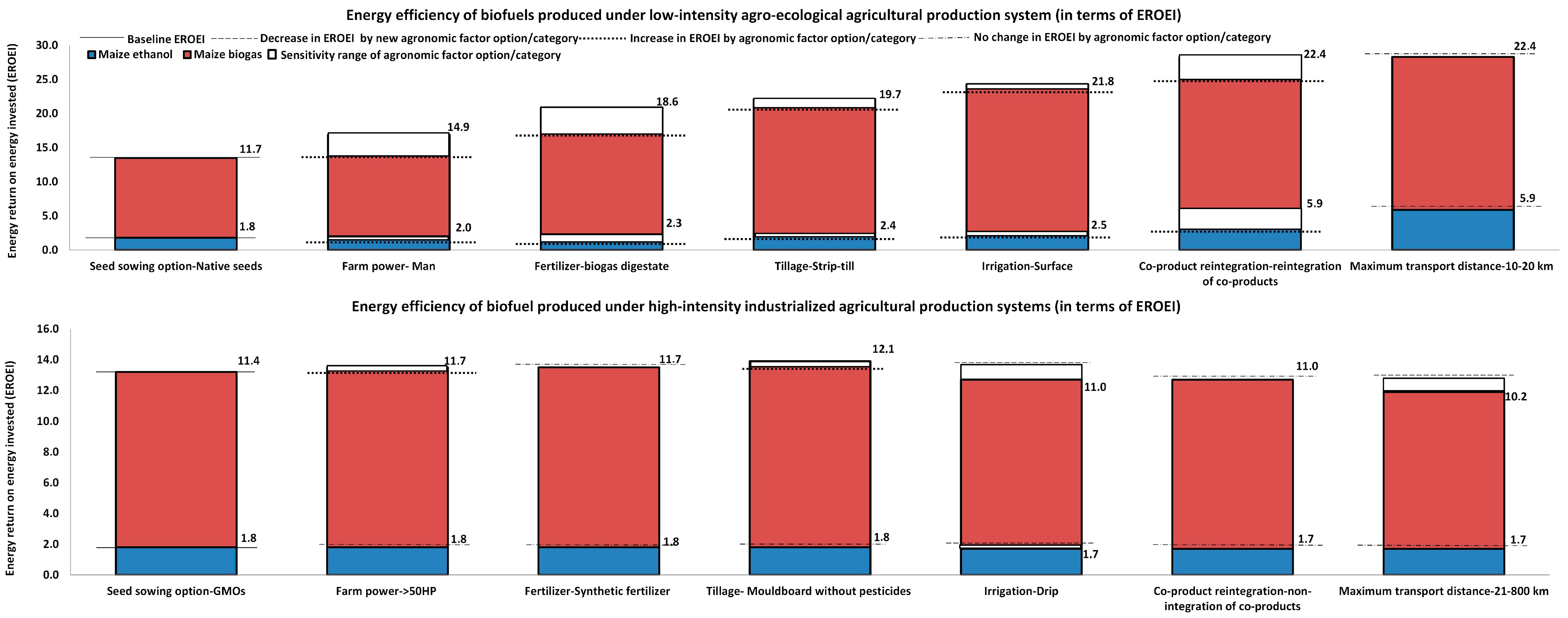
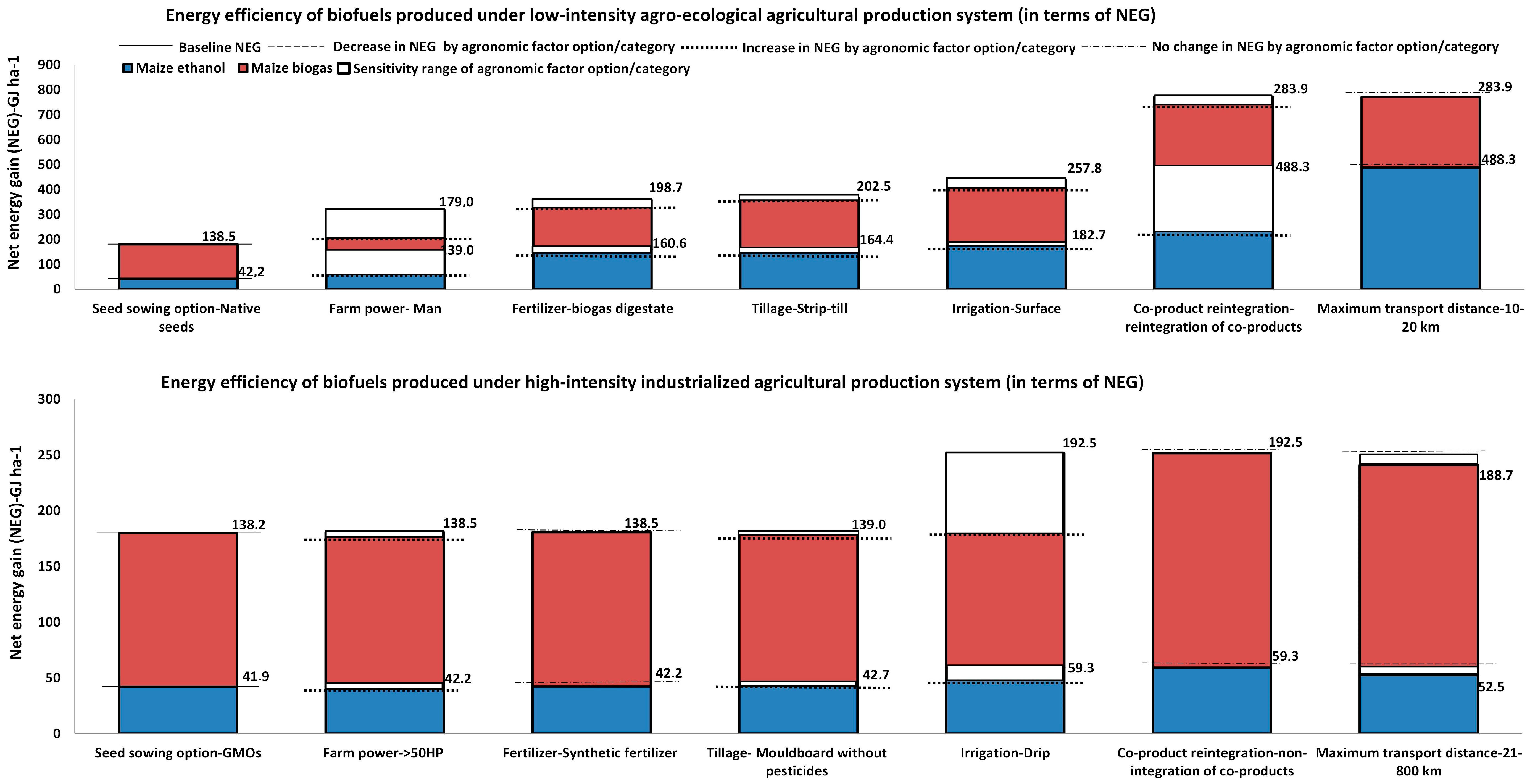
| Agronomic Factors | Effects on NEG | Effects on EROEI |
|---|---|---|
| Farm power (humans, animal and 10–20 HP tractors) | 12.5%–229.4% | 7.7%–27.4% |
| Tillage (reduced and no-till) | 4.2%–9.0% | 7.7%–9.4% |
| Fertilizer (animal manure and biogas digestate) | 3.1%–51.2% | 7.7%–31.6% |
| Irrigation (surface) | 39.9%–237.5% | 17.9%–40.0% |
| Co-product reintegration (biogas digestate, maize gluten meal) | 2.1%–724.2% | 2.5%–188.9% |
© 2016 by the authors; licensee MDPI, Basel, Switzerland. This article is an open access article distributed under the terms and conditions of the Creative Commons Attribution (CC-BY) license (http://creativecommons.org/licenses/by/4.0/).
Share and Cite
Arodudu, O.; Helming, K.; Wiggering, H.; Voinov, A. Bioenergy from Low-Intensity Agricultural Systems: An Energy Efficiency Analysis. Energies 2017, 10, 29. https://doi.org/10.3390/en10010029
Arodudu O, Helming K, Wiggering H, Voinov A. Bioenergy from Low-Intensity Agricultural Systems: An Energy Efficiency Analysis. Energies. 2017; 10(1):29. https://doi.org/10.3390/en10010029
Chicago/Turabian StyleArodudu, Oludunsin, Katharina Helming, Hubert Wiggering, and Alexey Voinov. 2017. "Bioenergy from Low-Intensity Agricultural Systems: An Energy Efficiency Analysis" Energies 10, no. 1: 29. https://doi.org/10.3390/en10010029
APA StyleArodudu, O., Helming, K., Wiggering, H., & Voinov, A. (2017). Bioenergy from Low-Intensity Agricultural Systems: An Energy Efficiency Analysis. Energies, 10(1), 29. https://doi.org/10.3390/en10010029