5.1. Full-Sample Analyses
First, we focus on Model (
5) to analyse the full-sample estimated parameters and their
p-values. This model was built to analyse and forecast the conditional quantiles of the FPC of the realized range-based bias corrected bipower variations. For simplicity,
Table 1 shows just the results associated with
; additional results for other quantiles are available on request. The standard errors are computed by means of a bootstrapping procedure using the
-pair method, which provides accurate results without assuming any particular distribution for the error term.
When τ equals 0.1, only is not significant at the 5% level. At , all the coefficients have small p-values, while for only is not significant. Finally, when , only and are highly significant. Therefore, the first important result is that the variables that significantly affect change according to the τ level. Notably, only is always significant, whereas is not significant only at . It is important to highlight that only and are significant in order to explain the high quantiles of volatility, which assume critical importance in finance. Moreover, the fact that is not significant for high values of τ is a reasonable result because the volatility is already in a ‘high’ state, and we might safely assume that the jump risk is already incorporated in it.
The fact that
and
are the most significant variables along the different quantiles’ levels is further confirmed when we compare two different models: a restricted model that has fewer explanatory variables (just
and
) against an unrestricted one that includes all the available covariates. The comparisons are made by means of the pseudo-coefficient of determination proposed by Koenker and Machado [
50], here denoted by
, and the test statistic
proposed by Koenker and Bassett [
51].
is a local goodness-of-fit measure, which ranges between 0 (when the covariates are useless to predict the response quantiles) and 1 (in the case of a perfect fit); with
, we aim to test the null hypothesis that the additional variables used in the unrestricted model do not significantly improve the goodness-of-fit with respect to the restricted model.
Table 2 shows the values of the pseudo-coefficient of determination computed for the restricted and the unrestricted models at
0.1, 0.2, 0.3, 0.4, 0.5, 0.6, 0.7, 0.8,
. We first observe that
is a positive function of
τ for both the models and then note that the differences between the restricted and the unrestricted models decrease as
τ increases, to substantially disappear at
. Therefore, the contribution of
,
and
to the goodness-of-fit of Model (
5) is largely irrelevant at
. We obtain similar conclusions from the test proposed in Koenker and Bassett [
51]: the null hypothesis of the test is not rejected at
, while at lower quantiles some of the additional variables provide sensible improvements in the model fit (see the fourth column of
Table 2).
Returning to the coefficients’ values, we note that the impact on the
conditional quantiles of
,
,
and
is positive in all cases in which the coefficients are statistically significant. Therefore, there is a positive relationship between these variables and
. With respect to the price jumps, the positive impact is a somewhat expected result, and it extends the findings in Corsi et al. [
52] about the impact of price jumps on realized volatility. However, as the coefficient of
,
, is always negative, in keeping with Black [
53], we find that an increasing market return implies greater stability and negative effects on
. We also checked on the persistence of volatility, measured by the sum of the HAR coefficients, that is,
, and noted that persistence is stronger at high levels of
τ:
,
and
. This evidence, which is coherent with the result for jumps, suggests that volatility in high regimes (upper quantiles) is more persistent as opposed to median or low regimes (lower quantiles) and that unexpected movements/shocks (including jumps) may have a larger effect on lower volatility quantiles compared to their impact on higher volatility quantiles, as they convey relevant information. While these results, recovered from a full-sample analysis, provide an interesting interpretation, they do not take into account the possible structural changes in the relationship between covariates and volatility conditional quantiles. This problem is analysed below.
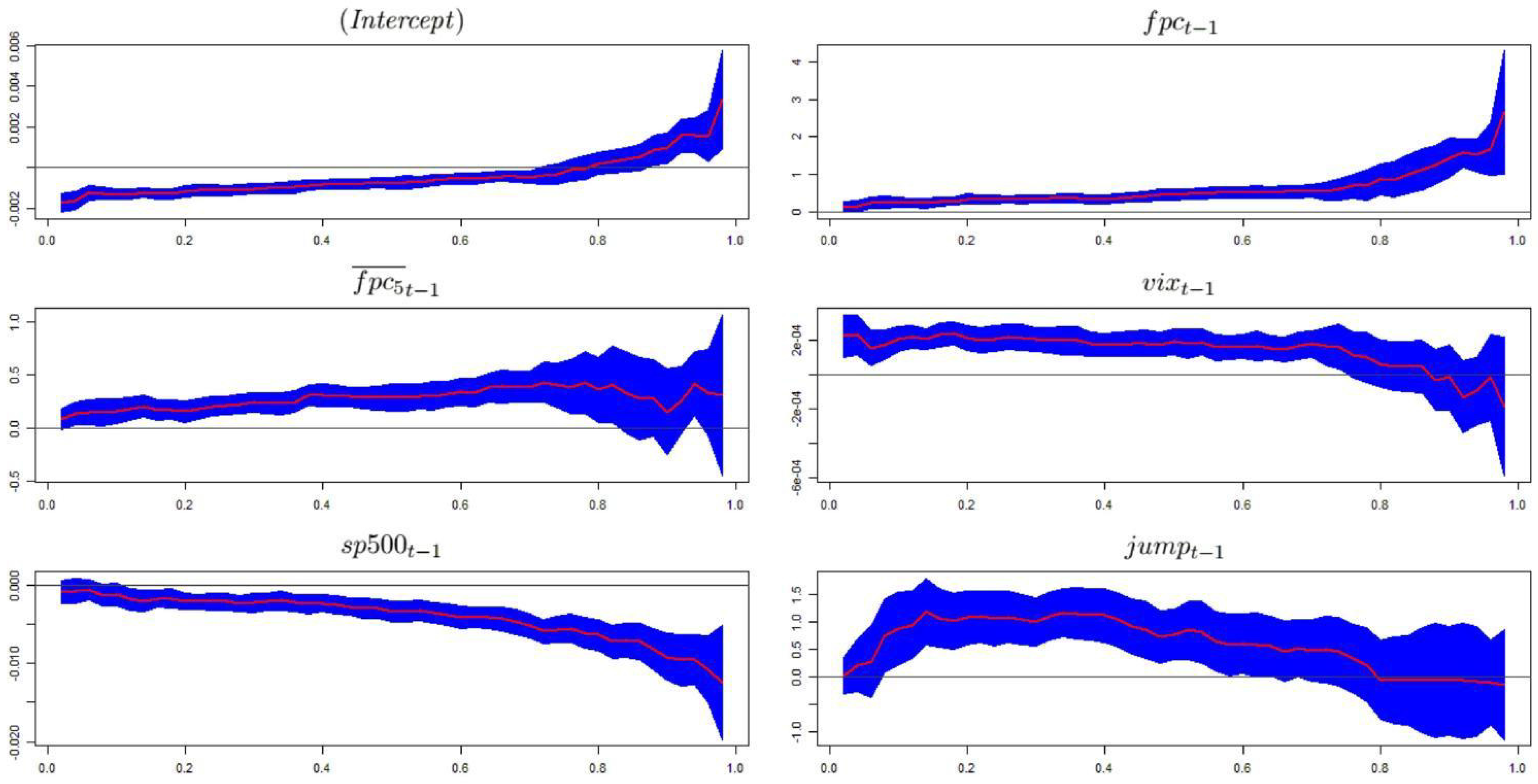
Even if the coefficients’ signs do not change over
τ, it is important to determine whether changes in
τ affect their magnitude. In other words, we want to check the so-called location-shift hypothesis, which states that the parameters in the conditional quantile equation are identical over
τ. Important information can be drawn from
Figure 1, which shows the coefficients’ plots.
The impact of
on the conditional quantiles of volatility is constant up to
, where it increases significantly. In the case of
, we observe a slightly increasing trend until
, when the uncertainty level becomes noticeable. The impact of
has a flat trend up to
, when it begins a decreasing trend, reaching negative values in a region where the regressor is not significant. However,
shows a negative effect on the volatility quantiles, and this relationship grows quickly at high values of
τ. We associate this finding with the so-called
leverage effect, as argued by Black [
53]: increases in volatility are larger when previous returns are negative than when they have the same magnitude but are positive. To verify this claim, we divided the
series into deciles and, conditional to those deciles, computed the mean of
for the various groups. As expected, the mean of
, corresponding to the values of
in the first decile, is 0.19%, whereas the mean corresponding to the last decile, in which we have the highest
values, is
%. As a consequence, the negative coefficients for
can be seen as supporting the existence of the leverage effect. Finally, in the case of
, we observe a wide band, where its impact grows at the beginning but takes negative turns from
.
To summarize, we verify that the relationships between the regressors and the response variable are not constant over τ. In particular, the impact of and grows considerably at high values of τ. Therefore, and are critical indicators in the context of extreme events where volatility can reach high levels. The coefficients of the other explanatory variables do not exhibit particular trends at low-medium levels of τ, and when τ assumes high values, they become even more volatile in a region of high uncertainty, given their wide confidence bands.
An analysis of the coefficients’ plots shown in
Figure 1 suggests that the hypothesis of equal slopes does not hold. To reach more accurate conclusions, we perform a variant of the Wald test introduced by Koenker and Bassett [
54]. The null hypothesis of the test is that the coefficient slopes are the same across quantiles. The test is performed taking into account three distant values of
τ,
, to cover a wide interval. When we compare the models estimated for
and
, the null hypothesis is rejected at the 95% confidence level for
,
and
. When we consider
and
, the null hypothesis is rejected at the 99% confidence level for
and
. We obtain the same result when we focus on
and
, so we have evidence against the location-shift hypothesis for those regressors. This finding confirms that the relationship between covariates and conditional quantiles varies across quantile values. This fundamentally relevant finding highlights that when the interest lies in specific volatility quantiles, linear models can lead to inappropriate conclusions about whether there is a relationship between covariates and volatility measures, and if there is, about the strength of the relationship.
5.2. Rolling Analysis
The U.S. subprime crisis and the European sovereign debt crisis have had noticeable effects on the financial system, with possible impacts also on the relationship between volatility and its determinants. Therefore, it is important to determine whether these events also affect the parameters of Model (
5). To this end, we perform a rolling analysis with steps of one day using a window size of 500 observations and
τ ranging from 0.05 to 0.95 with steps of 0.05. Therefore, we consider 19 levels of
τ and, for a given
τ, obtain 2133 estimates of a single coefficient. The finer grid adopted here allows us to recover a more accurate picture of the evolution of conditional quantiles. Nevertheless, the most relevant quantiles in this case are the upper quantiles, that are associated with the highest volatility levels. The estimated coefficients across time and quantiles are summarized in several figures.
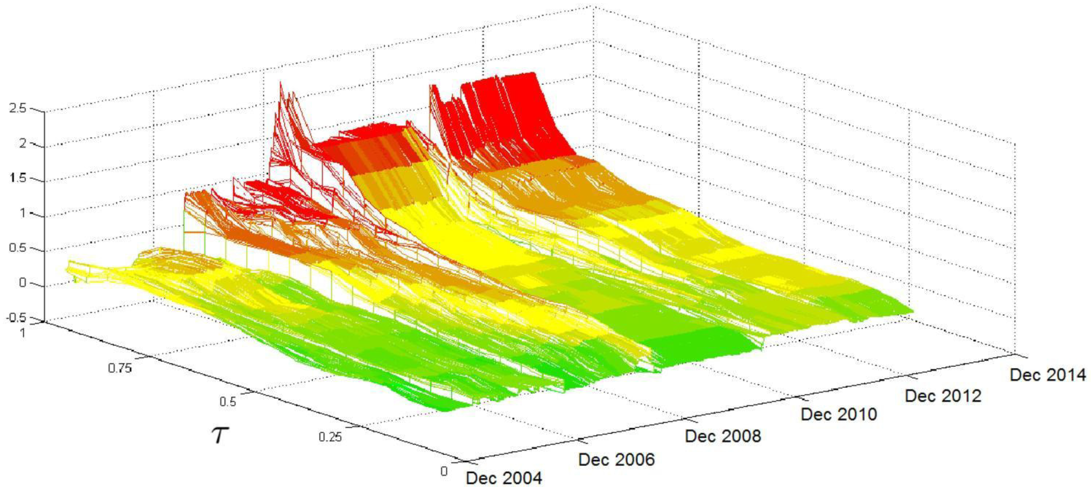
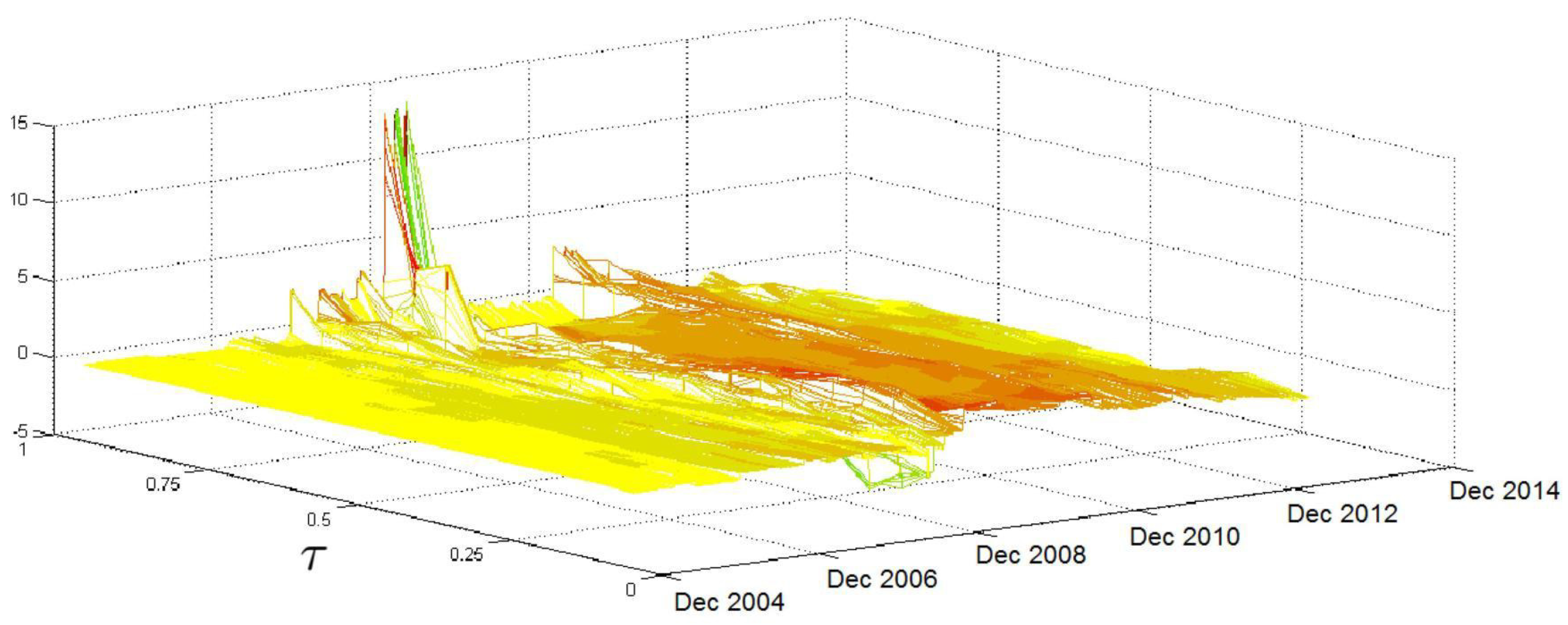
Figure 2 shows the evolution of the relationship between
and the conditional volatility quantiles over time and over
τ. The first result that arises from
Figure 2 is that the impact of
has a comparatively stable trend over time for medium-low
τ levels; some jumps are recorded, mainly in the period of the subprime crisis, but their magnitude is negligible. The picture significantly changes in the region of high
τ levels, where the surface is relatively flat and lies at low values in the beginning. However, after the second half of 2007, when the effects of the subprime crisis start to be felt, there is a clear increase in the coefficient values, which reach their peak in the months between late 2008 and the beginning of 2009. Moreover, in this period, we record the highest volatilities in the
coefficients over
τ levels. In the following months, the coefficient values decrease, but they remain at high levels until the end of the sample period.
is a highly relevant variable for explaining the entire conditional distribution of
because it is statistically significant over a large number of quantiles.
Figure 2 verifies that the relationship between
and
is affected by particular events, such as the subprime crisis, mainly at medium-high
τ levels. This finding confirms the change in the parameter across
τ values, with an increasing pattern in
τ and highlights that, during periods of market turbulence where the volatility stays at high levels, the volatility density overreacts to past movements of volatility, as the
coefficient is larger than one for upper quantiles. Therefore, after a sudden increase in volatility at, say, time
t, we have an increase in the conditional quantiles for time
and therefore an increase in the likelihood that we will observe additional volatility spikes (that is, volatility that exceeds a time-invariant threshold) at time
.
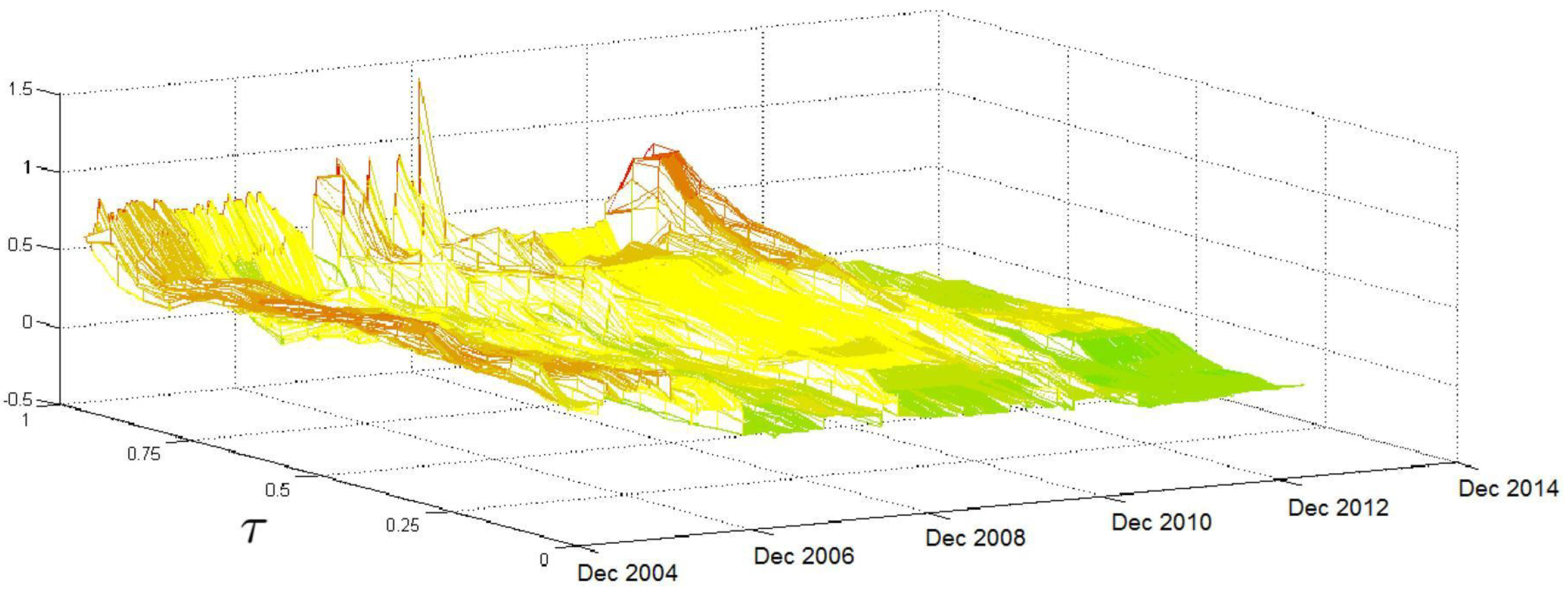
Referring to
, the HAR coefficient reported in
Figure 3 has a volatile pattern until late 2008, when it reaches its peak. After that, the surface flattens, but another jump is recorded in mid-2011, mainly in the region of high
τ values. Therefore, the relationship between the
quantiles and
, which reflects the perspectives of investors who have medium time horizons, is volatile over time, mainly in the region of high
τ values. Again, this result can be associated with crises that affect the persistence and the probability that extreme volatilities will occur.
Figure 4 shows two periods in which the
coefficient has high values: between the end of 2008 and early 2010 and a shorter period from the end of 2011 to the first half of 2012. While, in the first period, the impact of
significantly increases for all
τ levels; in the second period, the increase in the coefficient affects just the surface region in which
τ takes high values. Unlike the HAR coefficients described above, the
coefficient does not have a clear and stable increasing trend over
τ. In addition, the relationship between the
conditional quantiles and
is highly sensitive to the subprime crisis when pessimism among financial operators, reflected in the implied volatility of the S&P 500 index options, was acute. This result is again somewhat expected because we focus on U.S.-based data, and the subprime crisis had a high impact on the U.S. equity market. Our results are evidence that the perception of market risk has a great impact on the evolution of market volatility (as proxied by
), particularly during financial turmoil. The impact is not so clear-cut during the European sovereign crisis, which had less effect on the U.S. equity market.
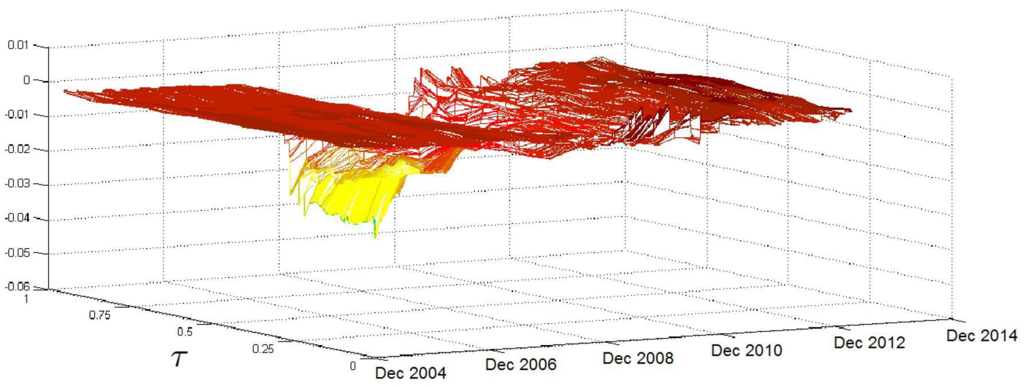
Figure 5 shows how the impact of
evolves over time and over
τ. The surface given is almost always flat, the exception being the months between late 2008 and the end of 2010, when the effects of the subprime crisis were particularly acute; during this time, the coefficient values decrease as
τ grows, mainly for values of
τ above the median. The lagged value of the S&P 500 index return affects the entire conditional distribution of
and is statistically significant in almost all the quantiles considered. Moreover,
Figure 5 shows that the effect is negative and particularly pronounced during the subprime crisis when negative returns exacerbated market risk, increasing the upper quantiles’ volatility and increasing the likelihood of large and extreme volatility events.
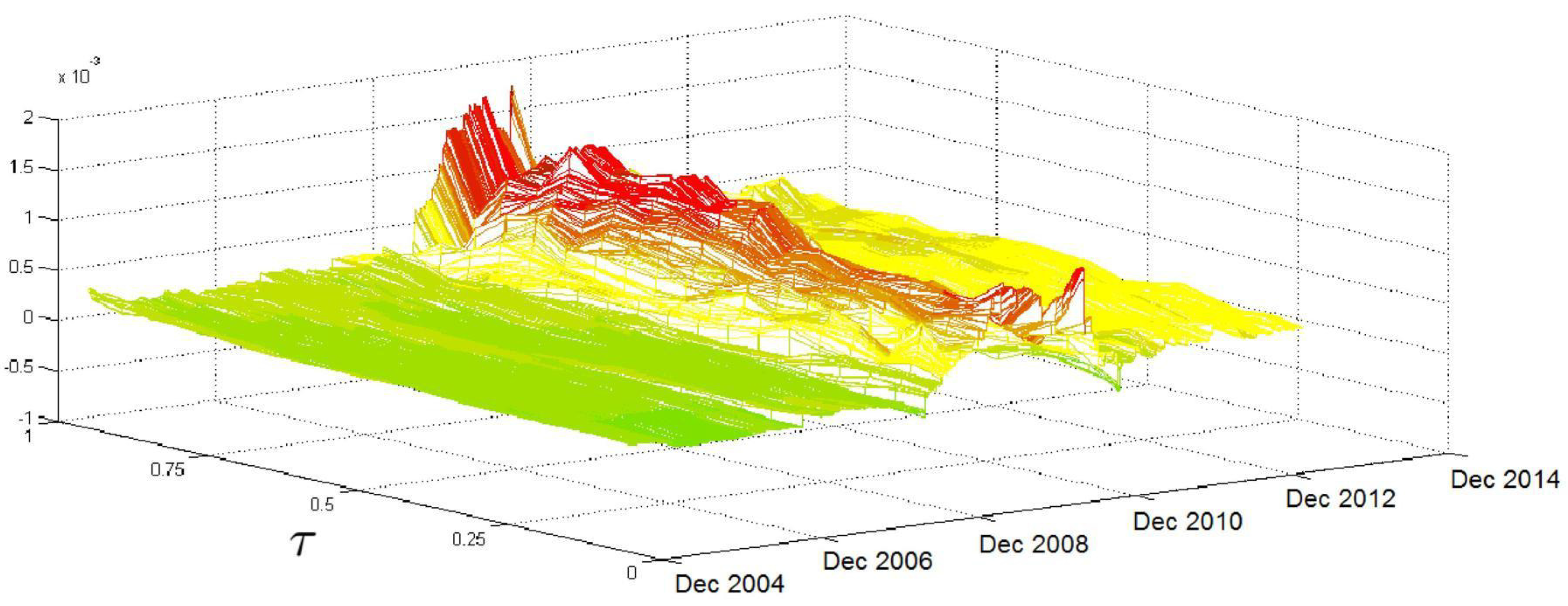
Finally,
Figure 6 shows the surface associated with the jump component. At the beginning of the sample, the
coefficient takes on small values over the
τ levels; however, it starts to grow in 2007, reaching high peaks at high
τ levels during the subprime crisis. Although the coefficient reaches considerable values in this region, their statistical significance is limited. After the second half of 2009, the surface flattens out again until the end of the sample, with the exception of some peaks of moderate size that were recorded in 2011 during the sovereign debt crises.
To summarize, using the rolling analysis, we show that two special and extreme market events (the U.S. subprime crisis and the European sovereign debt crisis) affected the relationships between the realized volatility quantiles and a set of covariates. Our results show that coefficients can reasonably vary, with a potential and relevant impact on the forecasts of both the mean (or median) volatility and the volatility distribution (starting from the quantiles). The effects differ across quantiles and change with respect to the volatility upper tails, as compared to the median and the lower tail. Therefore, when volatility quantiles are modeled, the impacts of covariates might differ over time and over quantiles, being crucial during certain market phases. This result further supports the need for quantile-specific estimations when there is an interest in single volatility quantiles.
5.3. Evaluation of the Predictive Power
We evaluate the volatility density forecasts using the tests of Berkowitz [
32], Amisano and Giacomini [
33] and Diebold and Mariano [
34]. We carry out the three tests by estimating a larger number of
conditional quantiles with respect to those analysed in
Section 5.2. This allows recovering more precise volatility distribution functions. In particular, we consider 49 values of
τ, ranging from 0.02 to 0.98, with steps of 0.02. Given the findings of the previous subsection, we must use a rolling procedure to build density forecasts. However, we modify the rolling scheme previously adopted to keep a balance between the reliability of the estimated coefficients and computational times. In particular, we recover the forecasts based on conditional quantiles estimated from subsamples of 100 observations, and we roll over the sample every 10 days. Within each 10-day window, we use fixed coefficients but produce one step-ahead forecasts updating the conditioning information set.
With regard to the Berkowitz test, in the case of Model (
5), we checked that
is normally distributed, as the likelihood ratio test
equals 5.26 and the null hypothesis of the Berkowitz test, that is,
with no autocorrelation, is not rejected at the 5% significance level, thus validating the forecast goodness of Model (
5). To determine whether the predictive power of our approach is affected by the U.S. subprime and the European sovereign debt crises, the series
is divided into two parts of equal length: the first referring to a period of relative calm, from the beginning of 2003 to the first half of 2007, and the second referring to a period of market turmoil that was due to the two crises between the second half of 2007 and the first half of 2013. In the first part,
equals 2.34, and in the second it equals 5.39. Nevertheless, the null hypothesis of the Berkowitz test is not rejected at the 5% level in both cases. Therefore, the conditional quantile model and the approach that we adopt to recover the conditional density forecasts are appropriate even during financial turbulence. An analysis of the results reveals that, as in the analysis of the full sample,
,
and
are not significant to explain the volatility quantiles at high values of
τ in many of the subsamples. Therefore, we must determine whether this result affects the output of the Berkowitz test using a restricted model in which the regressors are only
and
.
equals 2.60, a smaller value than in the previous cases. The last findings reported above suggest that the inclusion of non-significant explanatory variables penalizes the predictive power of Model (
5). The restricted model gives the lowest value of
, but the predictive power could be improved by selecting only those variables that are significant for each value of
τ and for each subsample to forecast the conditional distribution of the volatility. Thus, the structure of Model (
5) would change over time and over
τ. However, this approach is not applied in the present work because it would require using only the significant variables in 49 models, one for each specific value of
τ, while it should be considered across all the rolling subsamples.
So far, we have focused on an absolute assessment of our approach. Now, we compare it with a competing model that is fully parametric. We recover the predictive conditional distribution of the realized range volatility using a HARX model in which the mean dynamic is driven by a linear combination of the explanatory variables
and
(the HAR terms) and the exogenous variables
,
and
(the X in the model’s acronym). In addition, to capture the volatility-of-volatility effect argued by Corsi et al. [
31], a GJR-GARCH term [
30] is introduced to the innovation (we name the model HARX-GJR). The error term is also assumed to follow a normal-inverse Gaussian (
) distribution with a mean of 0 and a variance of 1. Thus, the conditional variance is allowed to change over time, and the distribution of the error is flexible in relation to features like fat tails and skewness. We start by using the Berkowitz test to evaluate the density forecast performance of the HARX-GJR model. The likelihood ratio test
equals 113.88, a high value that suggests a clear rejection of the null hypothesis. We also determined whether the HARX-GJR model works better when we use the logarithm of the volatility as a response variable, following the evidence in Corsi et al. [
52], and found that the likelihood ratio test
provides a much lower value (20.27). Even so, the test signals a rejection of the null hypothesis with a low
p-value. As a first finding, our approach provides more flexibility than the parametric HARX-GJR model does and is better in terms of the Berkowitz test.
To provide more accurate results, we move to a comparison of our approach to the HARX-GJR using the Amisano and Giacomini [
33] and the Diebold and Mariano [
34] tests. With regard to the Amisano and Giacomini [
33] test, we use four weights to compute the quantity given in Equation (
12):
,
,
and
. The associated likelihood ratio tests are denoted by
,
,
and
, respectively. Overall, our approach provides better results than the HARX-GJR because
is always positive; in fact,
,
,
and
. Given that the critical values at the 5% level are equal to
and 1.96 (we are dealing with a two-sided test), the null hypothesis of equal performance is rejected only when we give a higher weight to the right tail of the volatility conditional distribution.
Similar results are obtained when we consider the single quantile loss function and the Diebold and Mariano [
34] test statistic. Our approach provides lower losses because
is negative for all the
τ levels we considered (
). However, the differences are statistically significant only at
, given that
(0.0839),
(0.0831) and
(0.0072).
To summarize, the results demonstrate the good performance of our approach, in particular when we focus on the right tail of the FPC (a kind of market risk factor) distribution. We note that the right tail assumes critical importance in our framework, as it represents periods of extreme risks. Our findings indicate another relevant contribution of this study, as the quantile regression approach that we propose can be used to recover density forecasts for a realized volatility measure. These forecasts improve on those of a traditional approach because of the inclusion of quantile-specific coefficients. This feature of our approach might become particularly relevant in all empirical applications where predictive volatility density is required.
5.4. Single-Asset Results
The results in
Section 5.1,
Section 5.2 and
Section 5.3 were based on a summary of the 16 asset volatility movements, which was itself based on the FPC. Now, we search for confirmation of the main findings of Model (
5) by running Model (6) at the single-asset level for all 16 assets. For simplicity, only the results associated with
are shown (additional tables and figures relating to the single-asset estimates are available on request).
Table 3 provides the estimated parameters and their
p-values. We first focus on the relationships between
and
, for
. When
τ equals 0.1,
is not significant at the 5% level to explain the conditional volatility quantiles of eight assets:
,
,
,
,
,
,
and
. At
,
is not significant only for
, whereas, at
,
is not significant for
and
. Compared with the other regressors and in line with the results obtained for the FPC,
is one of the most significant explanatory variables at high levels of
τ, so it assumes critical importance in the context of extreme events. The
coefficient takes a negative value only for
at
, but here it is not statistically significant. In all the other cases, it is always positive. Moreover, the magnitude of the impact that
has on
is a positive function of
τ, for all 16 assets.
The differences among the assets increase as
τ grows, and at
the financial companies (
,
,
and
) record the highest coefficient values, highlighting the crucial importance of the extreme events in the financial system.
, the homologous regressor included in Model (
5), has a weaker impact on the conditional volatility quantiles than
does only for the financial companies
(
),
(
) and
(
). Therefore, the relationships between the conditional volatility quantiles and the lagged value of the response variable are stronger for the FPC than for the single assets.
is not significant (significance level of 0.05) at
for
,
and
, as the
p-values of its coefficient indicate. At
it is not significant only for
, whereas when
τ equals 0.9 it is not significant for
,
and
. The
coefficient is always positive and, with the exception of
and
, it is a positive function of
τ. Moreover, the differences among the
coefficient values are more marked at high
τ levels for all 16 assets. As for the comparison with the results obtained from Model (
5), at
,
has a stronger impact on the conditional volatility quantiles with respect to
for most of the 16 assets. When
τ equals 0.9, it is pointless to compare the coefficients’ values because
is not statistically significant at that level. Therefore, when we take into account the explanatory variables
and
, we record stronger relationships for Model (6) than for Model (5).
The p-values of the coefficient are less than 0.05 at for all 16 assets. When τ equals 0.9, is significant in the cases of , , , and . Unlike the coefficients previously mentioned, that of does not have a particular trend over τ; it takes positive values for all 16 assets, therefore, as in the context of the FPC, it has a positive impact on the conditional volatility quantiles. In addition, at , the coefficient of is larger in Model (5) than it is in Model (6) for all 16 companies. Therefore, has a more marked impact on the conditional volatility quantiles of the FPC. The comparisons made at are useless given the high p-values of the coefficients of interest.
is always significant () for the 16 assets, with the exception of , and at . Its coefficient is always negative, as expected, so has a negative impact on the conditional volatilities’ quantiles. In addition, the magnitude of the impact is a negative function of τ for all the assets, and those relationships become more marked at high τ levels. With the exception of one case ( at ), the impact of at is more pronounced for the conditional volatility quantiles of the FPC than it is when the assets are considered individually, as comparing the absolute values of the related coefficients shows.
At , is significant, at the 5% level, for , and . It is significant only for and at , whereas it is never significant when τ equals 0.9. ’s coefficient takes both negative and positive values and, with the exception of a few assets, it does not have a particular trend over τ. Comparing these results with those obtained for the conditional quantiles, we find that, with the exception of () and (), the lagged value of the component associated with jumps has more impact in Model (5) than in Model (6) at . It is pointless to compare the coefficients at given their high p-values.
To summarize, the explanatory variables , , and are sufficient to explain the conditional volatility quantiles of the 16 assets in most of the cases studied. Their coefficients tend to take the same sign for the 16 assets: positive in the cases of , and and negative in the case of . Moreover, the coefficients of , and have a clear trend over τ, providing evidence against the location-shift hypothesis, which assumes homogeneous impacts of the regressors across quantiles. However, is significant in only a few cases. Furthermore, with the exception of , we find that, in most of the studied cases, the relationships between the explanatory variables and the conditional volatility quantiles are more pronounced in the context of the FPC than when the assets are individually considered. This result shows that the FPC captures a kind of systematic effect, where the relationship between macro-level covariates, such as the VIX and the S&P 500 index, and volatility quantiles is clearer. At the single-asset level, the impact of covariates is more heterogeneous than for the FPC, perhaps suggesting the need for company- (or sector-) specific covariates.
The last point of our analysis refers to the assessment of the predictive power of Model (6), which we apply for each of the 16 assets. As in the case of the model for the FPC, we use the tests Berkowitz [
32], Amisano and Giacomini [
33] and Diebold and Mariano [
34] proposed. With regard to the Berkowitz test,
Table 4 provides the values of the likelihood ratio defined by Equation (
11) and the results generated by Model (6), showing that the null hypothesis of the test, that is,
with no autocorrelation, is not rejected for 10 assets:
,
,
,
,
,
,
,
,
and
. The results from the other six cases stem from the fact that some variables, mainly
, are not significant in many subsamples for several
τ levels. As indicated in
Section 5.3, which focused on the FPC, the predictive power of our approach could be improved by selecting for each subsample and each
τ only the regressors that are significant in order to explain the individually evaluated conditional quantiles. Thus, the structure of Model (6) would change over time. Now, we compare our approach with the HARX-GJR model. The results that arise from using the HARX-GJR model are given in
Table 4. As in the FPC context, the likelihood ratio test (11), denoted by
, takes high values for all 16 assets, suggesting that the null hypothesis is rejected with low
p-values.
Table 5 reports the results of the Amisano and Giacomini [
33] test and shows that overall our model provides better results: the test statistic values (
13) are in most cases positive, and the null hypothesis of equal performance is almost always rejected at the 5% level. Similar results are obtained for the Diebold and Mariano [
34] test, as we can see from
Table 6.
The sign of the test statistic (15) is always negative, suggesting that our approach implies a lower loss. Moreover, the performances are in most cases statistically different, given that the null hypothesis is often rejected at the 5% level. Therefore, the three tests provide clear evidence of the better performance of our method with respect to the benchmark and also in the case of single-asset realized volatilities.
To conclude, we found similar results for Models (5) and (6). In particular, for both models, the lagged value of the response variable and the lagged value of the S&P 500 return were fundamental explanatory variables at high τ levels, which are the most critical. In contrast, the lagged value of the jump component is significant in a few cases. We determined that the relationships between four explanatory variables (, , and ) and the conditional volatility quantiles are almost always stronger in Model (5) than in Model (6). However, in the case of , the relationships are stronger in Model (6) than in Model (5). Finally, even in the single-asset analysis, the goodness of the predicted power of our approach is validated using the three tests.


