Modelling the Effects of Oil Prices on Global Fertilizer Prices and Volatility

Abstract

The main purpose of this paper is to evaluate the effect of crude oil price on global fertilizer prices in both the mean and volatility. The endogenous structural breakpoint unit root test, ARDL model, and alternative volatility models, including GARCH, EGARCH, and GJR models, are used to investigate the relationship between crude oil price and six global fertilizer prices. The empirical results from ARDL show that most fertilizer prices are significantly affected by the crude oil price while the volatility of global fertilizer prices and crude oil price from March to December 2008 are higher than in other periods.

Introduction

The world population in 2000 was more than 6 billion, and is expected to reach 8 billion in 2025, based on projections by United Nation Population Division. The increase in global population, combined with economic development, will place increasing demand on agricultural food products, especially grains, rice, soybeans, and sugarcane. The derived demand for energy crops has been increased significantly due to the development of bio-fuel. Such development can lead to food shortages and increasing international food prices, which will encourage farmers to expand planted acreage. This predicament has increased the derived demand for global fertilizers and increased fertilizer prices.

Fertilizers are combinations of nutrients that enable plants to grow. The essential elements of fertilizers are nitrogen, phosphorus, and potassium. Urea fertilizer is the major fertilizer that provides the element of nitrogen, and is produced through converting atmospheric nitrogen using natural gas. Ammonia and phosphoric acid (hereafter ACID) are also produced using energy. Thus, prices for urea, ammonia, and ACID will be affected by crude oil prices. Monoammonium phosphate (hereafter MAP) and muriate of potash (hereafter MOP) are two other important fertilizers that are sources of phosphorus and potassium. As most of the world’s phosphate for fertilizer is mined, and hence is non-renewable, over the last decade the prices of phosphate and potash fertilizers have risen more steeply than the price of nitrogen-based urea.

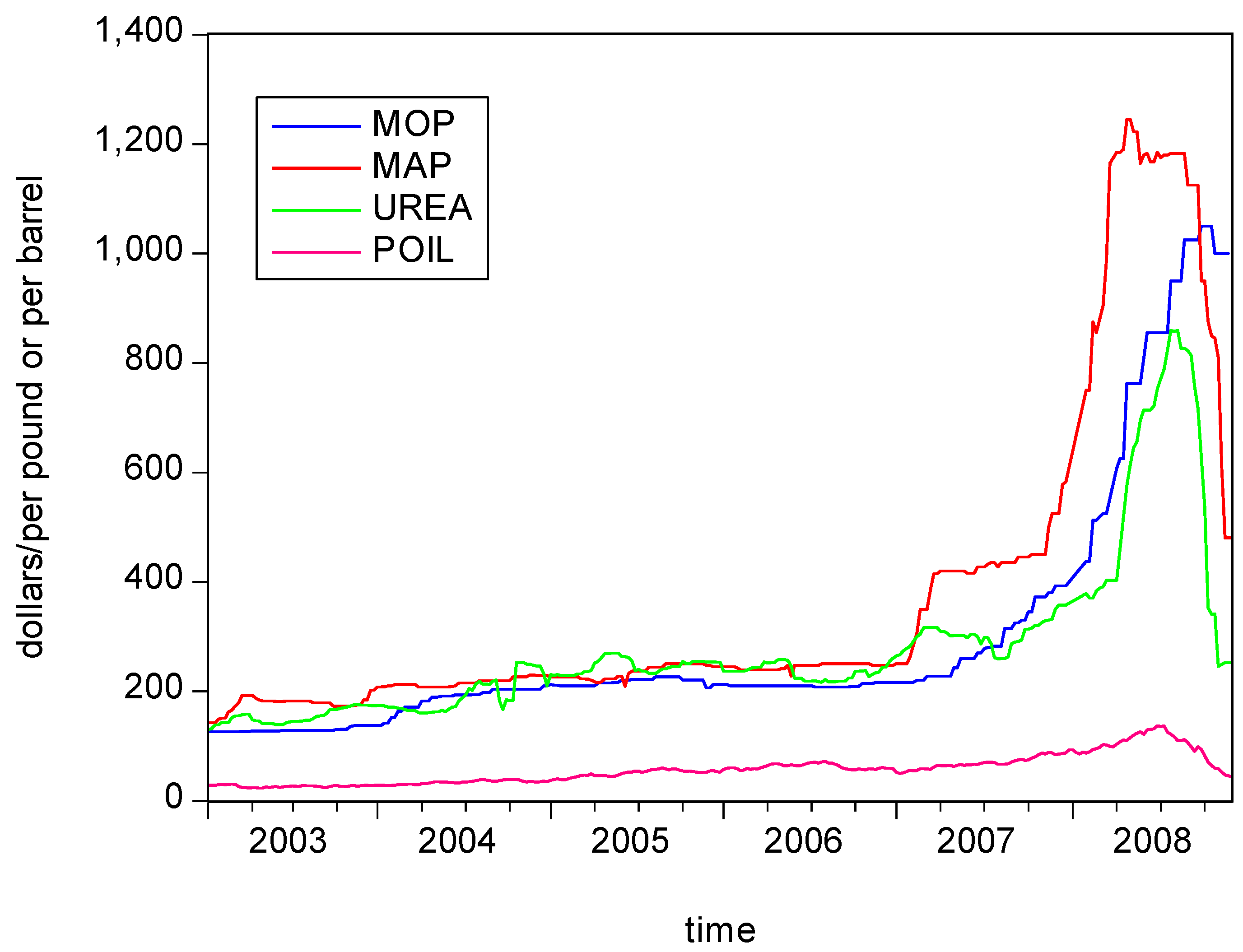
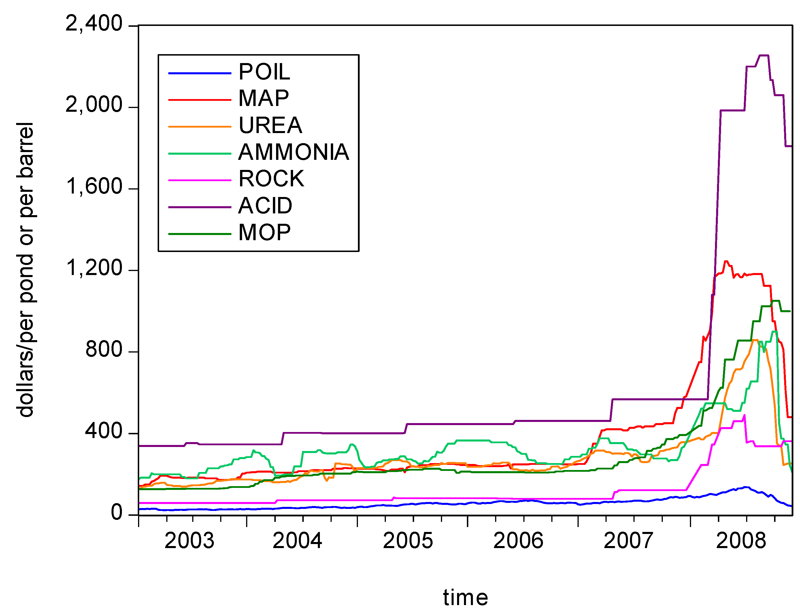
Figure 1 shows the trends in six fertilizer prices and Dubai crude oil price during the period 2003-2008. It is clear that most of these prices changed dramatically in 2007 and 2008. Figure 2 shows the trends in the prices of the main fertilizers, including MAP, MOP and urea, and Dubai crude oil weekly prices, from 2003-2008. This figure shows that fertilizers and Dubai crude oil price exhibit positive trends. Moreover, MAP and MOP prices had upsurge in early 2008. These figures show there is a clear positive relationship between global fertilizer prices and crude oil price. Therefore, the main purpose of this paper is to investigate the relationship between crude oil price and global fertilizer prices, in both the mean and volatility. As volatility invokes financial risk, such empirical results should provide useful information regarding the risks associated with variations in global fertilizer prices due to variations in oil price, with significant implications for optimal energy use, global agricultural production, and financial integration.

The remainder of the paper is organized as follows. Section 2 introduces the data, the empirical models are discussed in Section 3, and the empirical results are analyzed in Section 4. Some concluding remarks related to the energy policy implications of the volatility of global fertilizer prices are given in the final section.

2. Data

The source of the data is divided into two parts. The weekly global fertilizer supply prices are obtained from the Fertilizer Market Bulletin (hereafter FMB) weekly fertilizer report, while the weekly Dubai crude oil prices are obtained from the database in the Bureau of Energy during the period 2003-2008.

Table 1. Descriptive Statistics of Seven Price Series

Statistics	MAP (US$ /metric ton)	Urea (US$ /metric ton)	Ammonia (US$ /metric ton)	Acid (US$ /metric ton)	Rock (US$ /metric ton)	MOP (US$ /metric ton)	Poil (Price of Oil. US$/Bale)
Sample	254	254	254	254	254	254	254
Mean	258.07	225.80	280.72	428.30	78.46	206.18	48.29
Medium	237	234.50	278.25	445.00	79.50	210.00	51.56
Maximum	582.5	357.5	357.5	566.25	121.5	392.5	88.32
Minimum	142.5	50.5	176	338.5	58	126	22.97
Std. Dev.	89.39	55.51	53.89	70.01	18.97	57.95	17.23

gives the descriptive statistics of six fertilizer prices, including MAP, urea, ammonia, ACID, phosphate rock (hereafter ROCK), and MOP, and Dubai crude oil prices. The MAP prices show a steady upward trend, but have a sharp price spike in February 2008, as shown in Figure 1. The prices of urea and ammonia vary considerably, with steady increases over time. The ACID, ROCK, and MOP supply prices do not fluctuate significantly, but generally have upward trends. The trend in crude oil prices is relatively stable.

3. Model Specifications

Both the autoregressive distributed lag (ARDL) model and the generalized autoregressive conditional heteroskedasticity (GARCH) model will be used to evaluate the effects of oil and global fertilizer prices, and to model the volatility in global fertilizer and crude oil prices. Before estimating the ARDL and GARCH models, the Lee and Strazicich (2003) approach will be used to capture the structural breakpoint in fertilizer prices, which should enable identification of alternative time periods for the volatility in fertilizer prices.

3.1 Minimum LM unit root test with two endogenous breaks

Most traditional empirical studies use regression methods to estimate relationships among variables under the assumption of stationarity. However, spurious regression results may arise when some or all of the variables are non-stationary. The Dickey-Fuller (1979, 1981) test, Augmented Dickey-Fuller (ADF) test (1984), and Phillips-Perron test (1988) are widely-used unit root tests, but they are based on data generation processes with no structural breaks. Ignoring possible structural breaks can lead to non-rejection of the null hypothesis of non-stationarity, so that the effects of structural breaks may be attributed to the existence of a unit root. Nelson and Plosser (1982) used the Dickey-Fuller unit root test to examine U.S. macroeconomic time series, and found that widespread non-stationarity.

In order to tackle the problem of structural breaks, Perron (1989) proposed a unit root test with a structural breakpoint, which used an exogenous structural break to re-examine Nelson and Plosser’s (1982) data. The empirical results showed that most macroeconomic time series do not have unit roots, and the data features displayed by variables with a structural change are similar to those displayed by variables with unit roots. Thus, it is important to test for structural changes, otherwise an incorrect outcome of the unit root test is likely.

Banerjee et al. (1992) and Zivot and Andrews (1992) modified the unit root test with a known breakpoint to a unit root test with an unknown breakpoint. Lumsdaine and Papell (1997) and Lee and Strazicich (2003) transformed the unit root test with an unknown breakpoint into a unit root test with two unknown breakpoints. However, Lee and Strazicich (2003) establish minimum LM unit root test with two unknown structural change points to compensate for the shortcomings of the test. Both the null and alternative hypotheses are specified for series with two endogenous structural breakpoints.

3.2 Autoregressive Distributed Lag Model

Fertilizer can be divided into organic fertilizer and chemical fertilizer, with the latter being a high user of energy. For instance, nitrogen fertilizer production relies mainly on coal and natural gas, so that a causal relationship might be deemed to exist between crude oil and fertilizers prices. Such a relationship may be determined by a Granger Causality test and the autoregressive distributed lag (hereafter ARDL) model. The ARDL model, in which the data determine the short-run dynamics, would seem to be one of the most widely used models for estimating time series energy demand relationships (Jones, 1993; Benten and Engsted, 2001; Jones,1993; Benten and Engsted,2001; Dimitropoulos et al., 2005; Hunt et al., 2005; Hunt and Ninomiya, 2003; Chen et al.,2010).

Hendry(2005) indicates that the ARDL model merges dynamics and interdependence with different illustrations grounded by linear relationships. In this model, the price of a specific fertilizer is interpreted by the lags of itself price and crude oil prices. A general ARDL model for the global fertilizer price can be shown as bellow:

$$Fertilizer{P}_t={\alpha }_0+{\displaystyle \sum _{i=1}^p{\alpha }_{i}Fertilizer{P}_{t-i}+{\displaystyle \sum _{j=1}^q{\beta }_{j}Oil{P}_{t-j}}+}{u}_t$$

(1)

where $Fertilizer{P}_t$ is the global fertilizer price at time t, and $Oil{P}_t$ is the price of crude oil at time t.

The coefficient ${\beta }_j$ means the effect of the j-period lagged crude oil price on the fertilizer price, which implies that the fertilizer price can be predicted by the crude oil price. A test of the null hypothesis that each ${\beta }_j$ = 0 is a test of Granger non-causality.

All the variables included in the price should be stationary series to avoid spurious regression results, whereby the asymptotic standard normal results no longer hold. For this reason, the structural breakpoints of the crude oil price are estimated using the two-break minimum Lagrange Multiplier (LM) unit root test of Lee and Strazicich (2003). If and when the appropriate structural breakpoints are found, the fertilizer price equations will be estimated for different periods.

3.3 Conditional Mean and Conditional Volatility Models

Engle (1982) captured time-varying conditional volatility, or financial risk, through the autoregressive conditional heteroskedasticity (ARCH) model. Subsequent extensions, such as the generalized ARCH (GARCH) model of Bollerslev (1986), have been used to capture dynamic volatility for univariate and multivariate processes. The GARCH model is most widely used for symmetric shocks. In the presence of asymmetric shocks, whereby positive and negative shocks of equal magnitude have different impacts on volatility, the GJR model of Glosten et al. (1992) and the EGARCH model of Nelson (1991) are very useful. Further theoretical developments in specification, estimation and asymptotic theory have been suggested in Ling and Li (1997), Ling and McAleer (2002a, 2002b, 2003a, 2003b), and McAleer (2005).

The following model and discussion are based on McAleer (2005) and McAleer et al. (2007). The methods have been extended detect the volatility in patent growth by Chan et al. (2005a), in analyzing the volatility of USA ecological patents by Chan (2005b) and Marinova and McAleer (2003), in modelling the volatility of environment risk by Hoti et al. (2005), and the volatility of atmospheric carbon dioxide concentrations by McAleer and Chan (2006). However, there does not yet seem to have been any empirical analysis of such volatility models on global fertilizer prices, and hence no assessment of risk associated with such prices.

In this paper, we consider the stationary AR(1)-GARCH(1,1), or ARMA(p,q)-GARCH(1,1), model for the global fertilizer price series data, namely $y_t$:

$$\begin{gathered} y_t={\varphi }_1+{\varphi }_2{y}_{t-1}+{\epsilon }_t, \mathrm{for} t=1,...,n, \\ {y}_t=ARMA(p,q)+{\epsilon }_t \end{gathered}$$

(2)

where ${\epsilon }_t$ is the unconditional shock (or movement in global fertilizer prices), and is given by:

$$\begin{array}{l}{\epsilon }_t={\eta }_t\sqrt{h_t},{\eta }_t~iid(0,1),\\ h_t=\omega +\alpha {\epsilon }_{t-1}^2+\beta h_{t-1},\end{array}$$

(3)

and $\omega \ge$0,$\alpha \ge 0$,$\beta \ge 0$ are sufficient conditions to ensure that the conditional variance $h_t\ge 0$. Ling and McAleer (2003b) indicated equation (2) in the AR(1) process could be modified to incorporate a non-stationary ARMA(p,q) conditional mean and a stationary GARCH(r,s) conditional variance. In (2), the $\alpha$ (or ARCH) effect indicates the short run persistence of shocks, while the $\beta$ (or GARCH) effect indicates the contribution of shocks to long run persistence (namely, $\alpha +\beta$).

The parameters in equations (1) and (2) are typically estimated by the maximum likelihood method. Ling and McAleer (2003b) investigate the properties of adaptive estimators for univariate non-stationary ARMA models with GARCH(r,s) errors. The conditional log-likelihood function is given as follows:

$${\displaystyle \sum _{t=1}^n{l}_t}=-\frac{1}{2}{\displaystyle \sum _{t=1}^n(\log h_t+\frac{{\epsilon }_t^2}{h_t}})$$

As the GARCH process in equation (2) is a function of the unconditional shocks, the moments of ${\epsilon }_t$ need to be investigated. Ling and Li (2002a) showed that the ARCH(p,q) model is strictly stationary and ergodic if the second moment is finite, that is, ${(\alpha +\beta )}^2+2{\alpha }^2<1$. Ling and McAleer (2002b) showed that the Quasi MLE (QMLE) for GARCH(p,q) is consistent if the second moment is finite. Ling and Li (1997) demonstrated that the local QMLE is asymptotically normal if the fourth moment is finite, that is, $E({\epsilon }_t^4<\infty )$, while Ling and McAleer (2002b) proved that the global QMLE is asymptotically normal if the sixth moment is finite, that is, $E({\epsilon }_t^6<\infty )$. Using results from Ling and Li (1997), Bollerslev (1986), Nelson (1990), and Ling and McAleer (2002a, 2002b), the necessary and sufficient condition for the existence of the second moment of ${\epsilon }_t$ for GARCH(1,1) is $\alpha +\beta <1$ and, under normality, the necessary and sufficient condition for the existence of the fourth moment is ${(\alpha +\beta )}^2+2{\alpha }^2<1$.

For the univariate GARCH(p,q) model, several regularity conditions exist that enable the statistical validity of the model to be checked against the empirical data. Bougerol and Picard (1992) derived the necessary and sufficient condition, namely the log-moment condition or the negativity of a Lyapunov exponent, for strict stationarity and ergodicity (see Nelson (1990)). Using the log-moment condition, Elie and Jeantheau (1995) and Jeantheau (1998) established it was sufficient for consistency of the QMLE of GARCH(p,q) (see Lee and Hansen (1994) for the proof in the case of GARCH(1,1)), and Boussama (2000) showed that it was sufficient for asymptotic normality. Based on these theoretical developments, a sufficient condition for the QMLE of GARCH(1,1) to be consistent and asymptotically normal is given by the log-moment condition, namely

$$E(\log (\alpha {\eta }_t^2+\beta ))<0.$$

(4)

However, this condition is not straightforward to check in practice, even for the GARCH(1,1) model, as it involves the expectation of a function of a random variable and unknown parameters. The extension of the log-moment condition to multivariate GARCH(p,q) models has not yet been shown to exist, although Jeantheau (1998) showed that the ultivariate log-moment condition could be verified under the additional assumption that the determinant of the unconditional variance of ${\epsilon }_t$ in (1) is finite. Jeantheau (1998) assumed a multivariate log-moment condition to prove consistency of the QMLE of the multivariate GARCH(p,q) model. An extension of Boussama’s (2005b) log-moment condition to prove the asymptotic normality of the QMLE of the multivariate GARCH(p,q) process is not yet available.

The effects of positive shocks on the conditional variance,$h_t$, are assumed to be the same as the negative shocks in the symmetric GARCH model. In order to accommodate asymmetric behavior, Glosten et al. (1992) proposed the GJR model, for which GJR(1,1) is defined as follows:

$$h_t=\omega +(\alpha +\gamma I({\eta }_{t-1})){\epsilon }_{t-1}^2+\beta h_{t-1},$$

(5)

where $\omega >0$,$\alpha \ge 0$,$\alpha +\gamma \ge 0$,$\beta \ge 0$ are sufficient conditions for $h_t>0$ and $I({\eta }_t)$is an indicator variable defined by

$$I({\eta }_t)=\{\begin{array}{l}1\\ 0\end{array}\begin{array}{l}{\epsilon }_t<0.\\ {\epsilon }_t\ge 0,\end{array}$$

as ${\eta }_t$ has the same sign as ${\epsilon }_t$. The indicator variable differentiates between positive and negative shocks, so that asymmetric effects in the data are captured by the coefficient $\gamma$, with $\gamma \ge$0. The asymmetric effect, $\gamma$, measures the contribution of shocks to both short run persistence, $\alpha +\gamma /2$, and to long run persistence, $\alpha +\beta +\gamma /2$.

Ling and McAleer (2002b) derived the unique strictly stationary and ergodic solution of a family of GARCH processes, which includes GJR(1,1) as a special case, a simple sufficient condition for the existence of the solution, and the necessary and sufficient condition for the existence of the moments. For the special case of GJR(1,1), Ling and McAleer (2002b) showed that the regularity condition for the existence of the second moment under symmetry of ${\eta }_t$ is

$$\alpha +\beta +\frac{1}{2}<1,$$

(6)

and the condition for the existence of the fourth moment under normality of ${\eta }_t$ is

$${\beta }^2+2\alpha \beta +3\alpha +\beta \gamma +3\alpha \beta +\frac{3}{2}{\gamma }^2<1,$$

(7)

while McAleer et al. (2007) showed that the weaker log-moment condition for GJR(1,1) was given by

$$E(\ln [(\alpha +\gamma I({\eta }_t)){\eta }_t^2+\beta ])<0$$

(8)

which involves the expectation of a function of a random variable and unknown parameters.

An alternative model to capture asymmetric behavior in the conditional variance is the Exponential GARCH (EGARCH(1,1)) model of Nelson (1991), namely:

$$\log h_t=\omega +\alpha \left|{\eta }_{t-1}\right|+\gamma {\eta }_{t-1}+\beta \log h_{t-1},\left|\beta \right|<1$$

(9)

where the parameters $\alpha$, $\beta$ and $\gamma$ have different interpretations from those in the GARCH(1,1) and GJR(1,1) models.

As noted in McAleer et al. (2007), there are some important differences between EGARCH and the previous two models, as follows: (i) EGARCH is a model of the logarithm of the conditional variance, which implies that no restrictions on the parameters are required to ensure $h_t>0$; (ii) Nelson (1991) showed that $\left|\beta \right|<1$ ensures stationarity and ergodicity for EGARCH(1,1); (iii) Shephard (1996) observed that $\left|\beta \right|<1$ is likely to be a sufficient condition for consistency of QMLE for EGARCH(1,1); (iv) as the conditional (or standardized) shocks appear in equation (4), $\left|\beta \right|<1$ would seem to be a sufficient condition for the existence of moments; and (v) in addition to being a sufficient condition for consistency, $\left|\beta \right|<1$ is also likely to be sufficient for asymptotic normality of the QMLE of EGARCH(1,1).

Furthermore, EGARCH captures asymmetries differently from GJR. The parameters $\alpha$ and $\gamma$ in EGARCH(1,1) represent the magnitude (or size) and sign effects of the conditional (or standardized) shocks, respectively, on the conditional variance, whereas $\alpha$ and $\alpha +\gamma$ represent the effects of positive and negative shocks, respectively, on the conditional variance in GJR(1,1).

4. Empirical Results

4.1 Minimum LM unit root test with one and two breaks

The empirical results for the unit root tests, which are given in

Table 2. Augmented Dickey-Fuller (ADF) Unit Root Tests

Series	ADF tests
	With constant	With constant and trend	Critical values
			With trend	With constant and trend
Poil	-1.326(1)	-0.493(1)	-3.457 (1%) -2.873 (5%) -2.573 (10%)	-3.995 (1%) -3.428 (5%) -3.137 (10%)
MAP	-2.154(9)	-2.248(9)
Urea	-2.439(3)	-3.125(3)
Ammonia	-1.089(9)	-2.301(9)
Rock	-2.372(0)	-2.681(0)
Acid	-2.179(0)	-1.926(0)
MOP	3.280(0)	1.327(0)

Note: BIC is used to select the optimal lag length. The values in parentheses denote the number of lags.

, generally indicate that the ADF test does not reject the null hypothesis of a unit root. However, MAP, Urea, and ROCK reject the null hypothesis at the 1% significance level, which is consistent with no unit root for these prices, as shown in

Table 3. LM Unit Root Tests with Two Breaks

Series	LMτ	k	TB1	TB2
Poil	-6.017***	8	20071129	20080327
MAP	-8.239***	8	20071108	20080327
Urea	-8.264***	8	20071220	20080424
Ammonia	-5.775**	7		20080320
Rock	-7.926***	8	20070412	20080313
Acid	-15.920***	0	20071220	20080410
MOP	-9.549***	8	20071213	20080424

Notes: The 1%, 5% and 10% critical values are -5.823, -5.286, and -4.989, respectively (see Lee and Strazicich, 2003). *, ** and *** denote significance at the 10%, 5% and 1% levels, respectively.

, for the minimum LM unit root test with two breaks (see Lee and Strazicich (2003)). The price series for ammonia are tested using the minimum LM test unit root with one breakpoint as two breakpoints were not detected.

4.2 Granger Causality Test

As the results for testing the stationarity of the seven series indicate that all are stationary, we examine the relationships between the six fertilizer prices and the price of crude oil using the Granger Causality test (1969). From

Table 4. The Granger Causality test for six fertilizer prices with crude oil price

Dependent Variable	Period
	Period 1	Period 2	Period 3
MAP	4.030*	4.381*	4.958**
Urea	4.099*	4.743**	5.195**
Ammonia	3.429*	3.576*
Rock	0.336	1.086	0.477
Acid	4.040*	3.378*	3.622*
MOP	3.492*	3.183*	3.654*

Note: The value in table 4 belongs to F-Statistics. * and ** denote significance at the 5% and 1% levels, respectively.

, the crude oil price (given as Poil) is found to Granger-cause five fertilizer prices, namely MAP, urea, ammonia, ACID, and MOP, in each period, which indicates that oil prices can be used to predict these five fertilizer prices. However, the crude oil price does not Granger-cause the ROCK price at the 5% level of significance, which may not be so surprising as ROCK is a raw material used to produce phostate fertilizer, and hence does not use considerable energy. Thus, the oil price is not able to predict the ROCK price.

4.3 ARDL and Volatility Models for Crude Oil and Global Fertilizer Prices

The estimates of equation (1) for the MAP, urea, ammonia, ROCK, ACID and MOP prices are given in

Table 6. Mean and Volatility in MAP Prices

Period	2003/01/09-2007/11/01	2007/11/08-2008/03/20	2008/03/27-2008/12/04
Series (MAP)	ARMA (2,1)	ARMA (1,1)	ARMA (1,0)
	GARCH (1,1)	GARCH (1,1)	GARCH (1,1)
Mean Equation
AR (1)	0.633 (0.212)	0.848 (0.115)	0.819 (0.056)
AR (2)	-0.284 (0.122)
MA (1)	0.137 (0.064)	-0.228 (0.092)
Oil Price (-1)	0.236 (0.107)	0.636 (0.217)	0.613 (0.225)
Oil Price (-2)			0.280 (0.303)
Variance Equation
ω	0.768 (0.363)	0.015 (0.712)	0.032 (0.700)
α	0.108 (0.042)	0.288 (0.104)	0.387 (0.113)
β	0.275 (0.057)	0.266 (0.086)	0.469 (0.150)
γ
Log moment	-0.478	-0.373	-0.105
Second moment	0.385	0.554	0.856
Short run persistence	0.108	0.288	0.387
Long run persistence	0.385	0.554	0.856
BIC	5.465	8.169	7.610

Note: Values in parentheses denote standard errors.

,

Table 7. Mean and Volatility in Urea Prices

Period	2003/01/09-2007/12/13	2007/12/20-2008/04/17	2008/04/24-2008/12/04
Series (Urea)	ARMA (1,1)	ARMA (1,1)	ARMA (1,1)
	GARCH (1,1)	GARCH (1,1)	GARCH (1,1)
Mean Equation
AR (1)	0.675 (0.018)	0.756 (0.052)	0.779 (0.047)
MA (1)	-0.238 (0.088)	-0.183 (0.086)	0.050 (0.012)
Oil Price (-1)	0.806 (0.294)	3.114 (0.719)	2.897 (0.225)
Oil Price (-2)	0.531 (0.248)	1.958 (0.735)	1.493 (0.188)
Oil Price (-3)			0.574 (0.163)
Variance Equation
ω	0.452 (0.313)	0.647 (0.609)	0.094 (0.826)
α	0.059 (0.023)	0.364 (0.109)	0.312 (0.107)
β	0.272 (0.088)	0.279 (0.133)	0.595 (0.168)
γ
Log moment	-0.506	-0.259	-0.067
Second moment	0.331	0.643	0.907
Short run persistence	0.059	0.364	0.312
Long run persistence	0.331	0.643	0.907
BIC	6.485	6.853	6.305

Note: Values in parentheses denote standard errors.

,

Table 8. Mean and Volatility in Ammonia Prices

Period	2003/01/09-2008/03/13	2008/03/20-2008/12/04
Series (Ammonia)	ARMA (2,1)	ARMA (1,0)
	GARCH (1,1)	GARCH (1,1)
Mean Equation
AR (1)	0.883 (0.022)	0.788 (0.180)
AR (2)	-0.299 (0.022)
MA (1)	0.216 (0.040)
Oil Price (-1)	1.085 (0.318)	2.364 (0.489)
Oil Price (-2)	0.447 (0.212)	1.402 (0.315)
Variance Equation
ω	0.113 (2.494)	0.214 (1.130)
α	0.066 (0.025)	0.387 (0.112)
β	0.290 (0.038)	0.512 (0.245)
γ
Log moment	-0.472	-0.174
Second moment	0.356	0.899
Short run persistence	0.066	0.387
Long run persistence	0.356	0.899
BIC	7.238	7.568

Note: Values in parentheses denote standard errors.

,

Table 9. Mean and Volatility in Rock Prices

Period	2003/01/09-2007/04/05	2007/04/12-2008/03/06	2008/03/13-2008/12/04
Series (Rock)	ARMA (2,1)	ARMA (1,1)	ARMA (3,2)
	GARCH (1,1)	GARCH (1,1)	GARCH (1,1)
Mean Equation
AR (1)	0.334 (0.061)	0.963 (0.054)	0.703 (0.263)
AR (2)	0.248 (0.009)		-0.149 (0.107)
MA (1)	0.371 (0.061)	-0.223 (0.027)	0.279 (0.080)
MA (2)			0.106 (0.051)
Variance Equation
ω	0.005 (0.004)	0.121 (0.164)	0.160 (0.191)
α	0.109 (0.022)	0.262 (0.084)	0.369 (0.095)
β	0.327 (0.196)	0.359 (0.105)	0.442 (0.034)
γ
Log moment	-0.579	-0.436	-0.127
Second moment	0.436	0.621	0.811
Short run persistence	0.109	0.262	0.369
Long run persistence	0.436	0.621	0.811
BIC	1.751	2.611	2.558

Note: Values in parentheses denote standard errors.

,

Table 10. Mean and Volatility in Acid Prices

Period	2003/01/09-2007/12/10	2007/12/17-2008/03/31	2008/04/07-2008/12/04
Series (Acid)	ARMA (1.0)	ARMA (2,1)	ARMA (3,2)
	GARCH (1,1)	GARCH (1,1)	GARCH (1,1)
Mean Equation
AR (1)	0.648 (0.043)	0.695 (0.340)	0.793 (0.190)
MA (1)		0.113 (0.052)	0.101 (0.023)
Oil Price (-1)	0.214 (0.103)	1.053 (0.304)	0.628 (0.274)
Oil Price (-2)	0.131 (0.062)		0.325 (0.112)
Variance Equation
ω	0.401 (0.326)	0.038 (0.550)	0.329 (1.063)
α	0.059 (0.016)	0.203 (0.098)	0.298 (0.107)
β	0.257 (0.113)	0.227 (0.126)	0.463 (0.176)
γ
Log moment	-0.574	-0.323	-0.176
Second moment	0.316	0.430	0.694
Short run persistence	0.059	0.203	0.298
Long run persistence	0.316	0.430	0.694
BIC	7.222	7.475	7.202

Note: Values in parentheses denote standard errors.

and

Table 11. Mean and Volatility in MOP Prices

Period	2003/01/09-2007/12/06	2007/12/13-2008/04/17	2008/04/24-2008/12/04
Series (MOP)	ARMA (2,1)	ARMA (1,1)	ARMA (1,0)
	GARCH (1,1)	GARCH (1,1)	GARCH (1,1)
Mean Equation
AR (1)	0.830 (0.133)	0.899 (0.256)	0.896 (0.101)
AR (2)	-0.245 (0.107)
MA (1)	-0.122 (0.053)	-0.271 (0.129)
Oil Price (-1)	0.108 (0.036)	0.958 (0.273)	0.707 (0.234)
Oil Price (-2)	0.062 (0.020)		0.294 (0.151)
Variance Equation
ω	0.027 (0.028)	0.602 (0.476)	0.330 (0.571)
α	0.096 (0.032)	0.438 (0.163)	0.285 (0.116)
β	0.142 (0.014)	0.234 (0.114)	0.600 (0.266)
γ
Log moment	-0.738	-0.365	-0.101
Second moment	0.238	0.672	0.885
Short run persistence	0.096	0.438	0.285
Long run persistence	0.238	0.672	0.885
BIC	4.755	8.722	7.563

Note: Values in parentheses denote standard errors.

. Table 6 reports the estimates of crude oil price on MAP price for different periods. The coefficients of prices represent the change in the MAP price due to the change in the crude oil price. Similarly, the estimates of the price change for urea, ammonia, ACID, and MOP prices are reported in Table 7, Table 8, Table 9, Table 10 and Table 11, respectively. Owing to an insignificant causal relationship between ROCK price and crude oil price, we only estimate the volatility models for the ROCK price.

Several findings are given, as follows. The first main result is that the change in the lag one or two periods in the crude oil price has significant impacts on the prices of MAP, urea, ammonia, ACID, and MOP for the three time periods. For each fertilizer price, the effect of the crude oil price in the second and third periods is maintained at a higher level than in the first period. These empirical outcomes indicate that crude oil price and MAP, urea, ammonia, ACID, and MOP prices are more strongly related when the crude oil price is at a higher level, which is consistent with the observations in Figure 1 and Figure 2.

Another important issue to investigate is the effect on the five fertilizer prices due to a 1% change in the crude oil price, as implied in Table 6, Table 7, Table 8, Table 9, Table 10 and Table 11. Table 6. The percentage changes in fertilizer prices due to a 1% change in the crude oil price provide vital information concerning the sensitivity of each fertilizer price to changes in the oil price. For example, as shown in

Table 12. The Elasticity of Fertilizer Price with Respect to Crude Oil Price

The percentage change in each fertilizer price	a 1% changes in the crude oil price
	Period 1		Period 2		Period 3
MAP	Oil(-1)	1.252%	Oil(-1)	4.912%	Oil(-1)	6.416%
					Oil(-2)	2.931%
Urea	Oil(-1)	3.789%	Oil(-1)	15.445%	Oil(-1)	23.324%
	Oil(-2)	2.496%	Oil(-2)	9.711%	Oil(-2)	11.497%
					Oil(-3)	3.435%
Ammonia	Oil(-1)	6.265%	Oil(-1)	13.834%
	Oil(-2)	2.581%	Oil(-2)	8.205%
Acid	Oil(-1)	1.902%	Oil(-1)	7.929%	Oil(-1)	11.412%
	Oil(-2)	1.075%			Oil(-2)	6.530%
MOP	Oil(-1)	0.461%	Oil(-1)	4.914%	Oil(-1)	6.431%
	Oil(-2)	0.264%			Oil(-2)	2.674%

, the impact of the oil price on the MAP price is 1.252% in the first period, 4.912% in the second period, and 6.416% in the third period. Similar qualitative results are obtained for the effects of crude oil prices on the remaining four fertilizer prices.

The percentage changes in the five fertilizer prices due to a 1% change in the lagged values of crude oil price are positive in the second and third periods, but not in the first period, as the crude oil price has reached extremely high levels in the second and third periods. The oil price change is found to affect the price of fertilizer commodities through sharp increases in the prices of various energy-intensive inputs, including raw materials and fuel. This marked increase in the oil price is likely to have increased production costs. Consequently, the sensitivity of the five fertilizer prices to increases in the crude oil price become statistically significant when the crude oil price remains at a high level.

4.4 Alternative Volatility Models for Crude Oil and Six Global Fertilizer Prices

In order to investigate global fertilizer price volatility, an appropriate time series model needs to be determined that satisfies the appropriate regularity conditions. The first task is to determine the processes for the mean equation. We choose the ARMA processes with the smallest Schwarz Bayesian Information Criterion (BIC) value for the seven series in each period. The p-values of the Ljung-Box Q statistics of the residuals from the fitted models indicate that there is no autocorrelation at the 5% significance level. The specifications of the conditional mean and variance equations for the seven series are given in

Table 5. Volatility in Crude Oil Prices

Period	2003/01/09-2007/11/22	2007/11/29-2008/03/20	2008/03/27-2008/12/04
Series (Poil)	ARMA (3,2)	ARMA (2,1)	ARMA (3,3)
	GJR (1,1)	GJR (1,1)	GARCH (1,1)
Mean Equation
AR (1)	0.519 (0.062)	0.393 (0.016)	0.617 (0.030)
AR (2)	0.154 (0.007)	0.280 (0.002)	0.199 (0.010)
AR (3)	-0.181 (0.061)		0.032 (0.087)
MA (1)	0.473 (0.064)	-0.268 (0.065)	0.323 (0.011)
MA (2)	-0.753 (0.050)		-0.293 (0.013)
MA (3)			0.012 (0.077)
Variance Equation
ω	0.527 (0.178)	0.372 (0.164)	0.007 (0.014)
α	0.133 (0.034)	0.238 (0.085)	0.282 (0.031)
β	0.235 (0.108)	0.207 (0.199)	0.485 (0.079)
γ	-0.108 (0.075)	0.147 (0.096)
Log moment	-0.819	-0.598	-0.156
Second moment	0.421	0.519	0.768
Short run persistence	0.079	0.311	0.282
Long run persistence	0.314	0.519	0.768
BIC	2.491	3.814	4.601

Note: Values in parentheses denote standard errors.

, Table 6, Table 7, Table 8, Table 9, Table 10 and Table 11, respectively.

The appropriate volatility models for each of the six fertilizer prices and crude oil price are chosen on the basis of BIC and the regularity conditions, namely for the higher-order moments to exist, and hence for the asymptotic properties of consistency and asymptotic normality of the QMLE. The QMLE will be consistent and asymptotically normal when the weak log-moment condition is satisfied.

The empirical estimates for the alternative volatility models for the seven price series are given in Table 5, Table 6, Table 7, Table 8, Table 9, Table 10 and Table 11 for the three different time periods (that is, with. one or two structural breakpoints). Suitable models for Poil are GJR(1,1) for the first two periods, and GARCH(1,1) for the third period, as shown in Table 5. Periods 1 and 2 have asymmetric effects (with γ > 0 in the GJR(1,1) model). The short run persistence of shocks in periods 1, 2, and 3 are 0.079, 0.311 and 0.282, respectively, while the long run persistence of shocks in period 3 is 0.768, which is higher than in periods 1 and 2 of 0.314, and 0.519, respectively. These empirical outcomes indicate that a higher peak in the crude oil price is associated with greater volatility, which can be difficult to control. Thus, it is important for energy policy to understand the relationship between the prices and volatility of crude oil and global fertilizer prices.

For the MAP price series, a suitable model in three periods is GARCH(1,1), as shown in Table 6. The estimated coefficients satisfy the sufficient conditions for the conditional variance to be positive ($h_t\ge 0$). The short run persistence of shocks for MAP in periods 1, 2 and 3 is 0.108, 0.288 and 0.387, respectively, while long run persistence is 0.385, 0.554 and 0.856, respectively. Thus, MAP has the greatest long run persistence of shocks in the third period. As compared with both the short and long run persistence of the MAP and crude oil price, both price series have similar volatility effects in the three periods. In other words, both the level and volatility of MAP prices seem to be highly correlated with the crude oil price.

Table 7 shows that the GARCH(1,1) model is the appropriate model for the three periods for the Urea series. The estimates show that the weak log-moment condition is satisfied, so that the QMLE in the three periods for Urea are consistent and asymptotically normal. The short run persistence of shocks for Urea in periods 1, 2 and 3 is 0.059, 0.364 and 0.312, respectively, and the long run persistence of shocks in periods 1, 2 and 3 is 0.331, 0.643 and 0.907, respectively. The long run persistence of shocks in period 3 is greater than in the other two periods, which is similar to the case of the crude oil and MAP prices.

The appropriate model for the Ammonia series in the first and second periods is GARCH(1,1), as shown in Table 8. The short run persistence of shocks in periods 1 and 2 is 0.066 and 0.387, respectively, while the long run persistence of shocks in periods 1 and 2 is 0.356 and 0.899, respectively. The long run persistence of shocks in the second period is greater than its counterpart in period 1.

Appropriate volatility models for Rock, Acid, and MOP prices for the three different time periods are shown in Table 9, Table 10 and Table 11. For the Rock price series, the suitable model in the three time periods is GARCH(1,1), as shown in Table 9. For the Acid price series, as shown in Table 10, the best model in the three periods is GARCH(1,1). For the MOP price series, as shown in Table 11, the best model for all three time periods is GARCH(1,1).

The empirical results show that the long run persistence of shocks in periods 1, 2 and 3 is 0.436, 0.621 and 0.811, respectively, for the Rock price, so that the Rock price in period 3 has the greatest long run persistence of shocks. For Acid prices, the long run persistence of shocks in periods 1, 2 and 3 is 0.316, 0.430 and 0.694, respectively, so that the long run persistence in period 3 is the greatest. With regard to MOP prices, the long run persistence of shocks in the three periods is 0.230, 0.672 and 0.885, respectively, so that the third period again has the greatest long run persistence of shocks. Moreover, these price series behave in a similar manner to that of the crude oil price.

5. Concluding Remarks

The main purpose of the paper was to evaluate empirically the effect of crude oil price on global fertilizer prices, both in the mean and volatility. Weekly data for 2003-2008 were used in the empirical analysis. First, three time periods with two structural breakpoints were determined endogenously for six global fertilizer prices and crude oil price, using the Lee and Strazicich (2003) approach. Second, with regard to the relationships between the crude oil price and six global fertilizer prices, the Granger causality test showed that most global fertilizer prices are influenced by the crude oil price. The empirical results from the ARDL model showed that the percentage changes in five fertilizer prices (namely MAP, Urea, Ammonia, ACID, MOP) due to a 1% change in the crude oil price are relatively larger, and also statistically significant, in the second and third periods, which suggests that the oil price is an important factor in production costs for fertilizer commodities. Consequently, the sensitivity of the five fertilizer prices to the oil price increased, and became statistically significant. This also explains why global fertilizer prices reached a peak in 2008, as the crude oil price reached a high level in 2008.

An empirically adequate model of volatility of the six global fertilizer prices was determined by checking the regularity conditions of the estimated models. The symmetric and asymmetric univariate conditional volatility models, including the widely used GARCH, GJR and EGARCH models, were estimated and selected on the basis of the BIC criterion and the regularity conditions for the QMLE to be consistent and asymptotically normal. This is important for the empirical analysis, otherwise the empirical results would have no statistical foundation.

The contribution of shocks to the long run persistence of crude oil prices during the third period was found to be greater than during the first and second periods. This would suggest that the volatility in crude oil prices has recently increased in both strength and frequency. Therefore, the strength and frequency of global fertilizer prices has increased gradually over time. As the volatility in global fertilizer prices has increased, vital energy prices and global agricultural production are likely to be affected significantly. This may lead to future instability in agricultural food prices. These empirical findings are crucial for determining sensible energy policy in order to understand the directional relationship between the prices and volatility of crude oil and global fertilizer prices.

References

- A. Banerjee, R.L. Lumsdaine, and J.H. Stock. “Recursive and Sequential Tests for a Unit Root: Theory and International Evidence.” Journal of Business and Economic Statistics 10 (1992): 271–287. [Google Scholar]
- J. Benten, and T. Engsted. “A revival of the autoregressive distributed lag model in estimating energy demand relationships.” Energy 26 (2001): 45–55. [Google Scholar] [CrossRef]
- T. Bollerslev. “Generalized Autoregressive Conditional Heteroscedasticity.” Journal of Econometrics 31 (1986): 307–327. [Google Scholar] [CrossRef]
- P. Bougerol, and N. Picard. “Stationarity of GARCH Processes and of Some Non-Negative Time Series.” Journal of Econometrics 52 (1992): 115–127. [Google Scholar] [CrossRef]
- F. Boussama. “Asymptotic Normality for the Quasi-Maximum Likelihood Estimator of a GARCH Model.” Comptes Rendus de l’Academie des Sciences Série I 331 (2000): 81–84. (in French). [Google Scholar]
- F. Chan, D. Marinova, and M. McAleer. “Modelling Thresholds and Volatility in US Ecological Patents.” Environmental Modelling and Software 20 (2005): 1369–1378. [Google Scholar] [CrossRef]
- F. Chan, D. Marinova, and M. McAleer. “Rolling Regressions and Conditional Correlations of Foreign Patents in the USA.” Environmental Modelling and Software 20 (2005): 1413–1422. [Google Scholar] [CrossRef]
- S.T. Chen, H.I. Kuo, and C.C. Chen. “Modeling the Relationship between the Oil Price and Global Food Prices.” Applied Energy 87 (2010): 2517–2525. [Google Scholar] [CrossRef]
- D.A. Dickey, and W.A. Fuller. “Distribution of the Estimators for Autoregressive Time Series with a Unit Root.” Journal of the American Statistical Association 74 (1979): 427–431. [Google Scholar]
- D.A. Dickey, and W.A. Fuller. “Likelihood Ratio Statistics for Autoregressive Time Series with a Unit Root.” Econometrica 49 (1981): 1057–1072. [Google Scholar] [CrossRef]
- J. Dimitropoulos, L.C. Hunt, and G. Judge. “Estimating underlying energy demand trends using UK annual data.” Applied Economics Letters 12 (2005): 239–244. [Google Scholar] [CrossRef] [Green Version]
- L. Elie, and T. Jeantheau. “Consistency in Heteroskedastic Models.” Comptes Rendus de l’Académie des Sciences Série I 320 (1995): 1255–1258. (in French). [Google Scholar]
- R.F. Engle. “Autoregressive Conditional Heteroskedasticity with Estimates of the Variance of United Kingdom Inflation.” Econometrica 50 (1982): 987–1007. [Google Scholar] [CrossRef]
- FAO. “Current World Fertilizer Trends and Outlook to 2012.” 2008. Url: ftp://ftp.fao.org/agl/agll/docs/cwfto12.pdf.
- FAPRI UMC report. “Fertilizer and Fuel Prices and Cost of Production.” 2004. Url: http://www.fapri.missouri.edu/outreach/publications/2004/FAPRI_UMC_Report_10_04.pdf.
- L. Glosten, R. Jagannathan, and D. Runkle. “On the Relation Between the Expected Value and Volatility of Nominal Excess Return on Stocks.” Journal of Finance 46 (1992): 1779–1801. [Google Scholar] [CrossRef]
- C.W.J. Granger. “Investigation Causal Relations by Econometric Models and Cross-spectral Methods.” Econometrica 37 (1969): 424–438. [Google Scholar] [CrossRef]
- D.F. Hendry. Dynamic Econometrics: Advanced Text in Econometrics. Oxford: Oxford University Press, 1995. [Google Scholar]
- S. Hoti, M. McAleer, and L. Pauwels. “Modelling Environmental Risk.” Environmental Modelling and Software 20 (2005): 1289–1298. [Google Scholar] [CrossRef]
- L.C. Hunt, G. Judge, and Y. Ninomiya. “Underlying trends and seasonality in UK energy demand: a sectoral analysis.” Energy Ecnomics 25, 1 (2003): 93–118. [Google Scholar] [CrossRef]
- L.C. Hunt, and Y. Ninomiya. “Primary Energy Demand in Japan: An Empirical Analysis of Long-term Trends and Future CO2 Emissions.” Energy Policy 33, 11 (2005): 1409–1424. [Google Scholar] [CrossRef]
- T. Jeantheau. “Strong Consistency of Estimators for Multivariate ARCH Models.” Econometric Theory 14 (1998): 70–86. [Google Scholar] [CrossRef]
- C.T. Jones. “A Single-equation Study of U.S. Petroleum Consumption: the Role of Model Specification.” Southern Economic Journal 59, 4 (1993): 687–700. [Google Scholar] [CrossRef]
- J. Lee, and M.C. Strazicich. “Minimum Lagrange Multiplier Unit Root Test with Two Structural Breaks.” Review of Economics and Statistics 85 (2003): 1082–1089. [Google Scholar] [CrossRef]
- S.W. Lee, and B.E. Hansen. “Asymptotic Theory for the GARCH(1,1) Quasi-Maximum Likelihood Estimator.” Econometric Theory 10 (1994): 29–52. [Google Scholar] [CrossRef]
- S. Ling, and W.K. Li. “On Fractionally Integrated Autoregressive Moving-Average Models with Conditional Heteroskedasticity.” Journal of the American Statistical Association 92 (1997): 1184–1194. [Google Scholar] [CrossRef]
- S. Ling, and M. McAleer. “Stationarity and the Existence of Moments of a Family of GARCH Processes.” Journal of Econometrics 106 (2002): 109–117. [Google Scholar] [CrossRef]
- S. Ling, and M. McAleer. “Necessary and Sufficient Moment Conditions for the GARCH(r,s) and Asymmetric Power GARCH(r,s) Models.” Econometric Theory 18 (2002): 722–729. [Google Scholar] [CrossRef]
- S. Ling, and M. McAleer. “Asymptotic Theory for a Vector ARMA-GARCH Model.” Econometric Theory 19 (2003): 278–308. [Google Scholar] [CrossRef]
- S. Ling, and M. McAleer. “On Adaptive Estimation in Nonstationary ARMA Models with GARCH Errors.” Annals of Statistics 31 (2003): 642–674. [Google Scholar]
- R. Lumsdaine, and D. Papell. “Multiple Trend Breaks and the Unit Root Hypothesis.” Review of Economics and Statistics 79 (1997): 212–218. [Google Scholar] [CrossRef]
- D. Marinova, and M. McAleer. “Modelling Trends and Volatility in Ecological Patents in the USA.” Environmental Modelling and Software 18 (2003): 195–203. [Google Scholar] [CrossRef]
- M. McAleer, and F. Chan. “Modelling Trends and Volatility in Atmospheric Carbon Dioxide Concentrations.” Environmental Modelling and Software 20 (2006): 1273–1279. [Google Scholar] [CrossRef]
- M. McAleer, F. Chan, and D. Marinova. “An Econometric Analysis of Asymmetric Volatility: Theory and Application to Patents.” Journal of Econometrics 139 (2007): 259–284. [Google Scholar] [CrossRef]
- M. McAleer. “Automated Inference and Learning in Modeling Finanical Volatility.” Econometric Theory 21 (2005): 232–261. [Google Scholar] [CrossRef]
- C.R. Nelson, and C.I. Plosser. “Trends and random walks In Macroeconomic Time Series.” Journal of Monetary Economics 10 (1982): 139–162. [Google Scholar] [CrossRef]
- D.B. Nelson. “Conditional Heteroscedasticity in Asset Returns: A New Approach.” Econometrica 59 (1991): 347–370. [Google Scholar] [CrossRef]
- D.B. Nelson. “Stationarity and Persistence in the GARCH(1,1) Model.” Econometric Theory 6 (1990): 318–334. [Google Scholar] [CrossRef]
- P. Perron. “The Great Crash, the Oil Price Shock and the Unit Root Hypothesis.” Econometrica 57 (1989): 1361–1401. [Google Scholar] [CrossRef]
- P.C.B. Phillips, and P. Perron. “Testing for a unit root in time series regression.” Biometrika 75 (1988): 335–346. [Google Scholar] [CrossRef]
- S. Said, and D. Dickey. “Testing for unit roots in autoregressive moving average models with unknown order.” Biometrika 71 (1984): 599–607. [Google Scholar] [CrossRef]
- N. Shephard. “Statistical Aspects of ARCH and Stochastic Volatility.” In Time Series Models in Econometrics, Finance, and Other Fields. Edited by D.P. Cox, O.E. Barndorff-Nielsen and D.V. Hinkley. London: Chapman and Hall, 1996, pp. 1–67. [Google Scholar]
- E. Zivot, and D.W.K. Andrews. “Further Evidence on Great Cash, the Oil Price Shock and the Unit Root Hypothesis.” Journal of Business and Economic Statistics 10: 251–270.
Figure 1.
Price Trends for Global Fertilizers and Crude Oil, 2003-2008
Figure 2.
Higher Energy Use Fertilizer Prices and Crude Oil Price, 2003-2008