1. INTRODUCTION
Options pricing and management of derivative positions are an important area of finance. The derivatives market is now also very large. According to recent estimates by BIS Quarterly Review (2011) as at June 2011, the notational amount of outstanding option OTC derivative contracts was 78.8 trillion US dollars. As such, options and other derivative instruments are traded extensively on many global exchanges by hedgers, speculators and arbitrageurs. The derivative markets play a key role in the transfer of risk between these different parties.
The development of the Black-Scholes option pricing model and its equivalent binomial option pricing model represented a major breakthrough in the pricing of corporate stock options (Black and Scholes, 1973; Merton, 1973; and Cox, Ross and Rubenstein, 1979). Since the development of the Black-Scholes and binomial models there have been numerous refinements to the models to account for stock dividends (Merton, 1973), American style options (Barone-Adesi and Whaley, 1986, 1987), foreign exchange options (Garman and Kohlhagen, 1983) and other more exotic options (Hull, 2011). The Black-Scholes option pricing model assumes prices follow a geometric Brownian motion and volatility is constant. A number of authors have also attempted to modify the Black-Scholes and binomial option pricing models to allow for stochastic and time varying volatility (Cox and Ross, 1976). Other adjustments to the Black-Scholes model include models where jumps are superimposed on a continuous return change (e.g. Merton, 1976).
A problem with any option pricing model is the estimation of the parameter inputs and in particular the ex-ante volatility. In this paper we examine if a Bayesian estimate of volatility can provide a better estimate of ex-ante stock price volatility compared to a simple historical volatility estimate, as an input into the Black-Scholes and binomial option pricing models. Specifically, we compare the difference between both Bayesian and historical volatility estimates to the underlying implied stock price volatility. Our implied volatility estimates are supplied by IVolatility and calculated from publicly traded call and put option prices using the binomial option pricing model.
Despite numerous variants to the Black-Scholes model and the binomial options pricing model, these models still remain extensively used in practice. For instance, International Financial Reporting Standard No 2 notes that valuers may use the Black-Scholes/ binomial options pricing model, or variants thereof, to price employee stock options that must now be expensed in accordance with international financial reporting rules. Similarly, since December 2004, Statement of Accounting Concepts 123R issued by the Financial Accounting Standards Board, requires firms to recognise the value of employee stock options in their financial statements. In a study of the comparative inputs to estimate the fair value of employee stock options, Choudhary (2011) reported that 96% of her sample of US firms used the Black-Scholes model, 4% used the binomial options pricing model and 0.3% used an unspecified model. Similarly Balsam et al. (2007) reported that 86% of firms surveyed in their study used the Black-Scholes model. In practice, valuers and option traders that use the Black-Scholes or binomial option pricing models often adjust the standard models to account for a volatility smile in the pricing of stock options with different exercise prices (Hull, 2011).
1In summary, despite its well-documented shortcomings, the use of the Black-Scholes and the simple binomial option pricing models to price options remains widespread. Therefore, as noted by Darsinos and Satchell (2007), it is of interest to investigate how the Black-Scholes and binomial models might be improved, while still retaining their essential simplicity. An obvious possibility for improvement is to refine the estimate of volatility, within the Black-Scholes assumption of a geometric Brownian motion for the underlying asset, or equivalently of a random walk for the log price. Although this assumption is not precisely satisfied, as already noted, the Black-Scholes and binomial model formula is regarded to be sufficiently robust to departures from this assumption to still be extensively used, despite the plethora of more sophisticated models that have been proposed.
In this paper, we provide a relatively simple method to estimate volatility using a Bayesian approach that can be applied in practice as an alternative to using historical volatility as a proxy for ex-ante volatility. A more reliable estimate of ex-ante volatility compared to historical stock price volatility may be useful to price options on stocks that have no existing options traded and where an implied volatility estimate cannot be observed. As in Karolyi (1993) and Darsinos and Satchell (2007), we find that use of the Bayes estimate represents an improvement over the historical volatility. A feature of these two papers is the use of an inverse gamma prior for the volatility parameter. However, as we demonstrate in
Section 3, the actual distribution of 30-day volatilities for the sample of stocks that we examine is much better modelled by a gamma distribution (or mixture of gammas) rather than an inverse gamma distribution, and use of this prior leads to a better estimate.
Our finding that Bayesian volatility estimates outperform historical volatility estimates in the determination of an implied volatility estimate will therefore be of interest to both practitioners and academics.
The remainder of this paper is structured as follows.
Section 2 reviews the prior literature.
Section 3 describes our data.
Section 4 develops the mathematical framework to determine our Bayesian volatility estimates.
Section 5 compares the differences in errors between the historical and our Bayesian option volatility estimates compared to the implied option volatility sourced from IVolatility.
Section 6 concludes.
2. PRIOR RESEARCH
A Bayesian framework has previously been employed in finance literature by Vasicek (1973) to estimate beta in the capital asset pricing model and hence determine a company’s cost of equity capital. Elton et al. (1978), Eubank and Zumwalt (1979), Blume (1975) and Klemkosky and Martin (1975) empirically show that a Bayesian estimate of beta in the capital asset pricing model provided a better estimate of beta than the traditional estimate of beta.
Several authors have also applied Bayesian methods to the estimation of stock price volatility in connection with pricing options, both under the assumption of geometric Brownian motion and under more complicated models for time-varying volatility. For example, Bauwens and Lubrano (2002) assume that the underlying asset follows a GARCH process and apply Bayesian methods to the calculation of option prices. Martin, Forbes and Martin (2005) and Flynn, Grose, Martin and Martin (2005) also assume a GARCH model for the underlying asset, and derive the form of the risk-neutral probability density q(θ). They use observed option prices to estimate the posterior distribution of the parameters θ. Forbes, Martin and Wright (2007) develop a joint model for the asset price and the option price, again using observed option prices. Jacquier and Jarrow (2000) use regression models linking the option price to the asset price. In work more in the spirit of ours, Karolyi (1993) and Darsinos and Satchell (2007) assume a random walk model for the asset price and present a Bayesian analysis, assuming a normal model for the log-returns and an inverse gamma prior on the volatility.
A number of studies have examined if implied or historical volatility estimates provide a better forecast estimate of future realised volatility. Early studies on Chicago Board Options Exchange data for stocks by Latane and Rendleman (1976), Chiras and Manaster (1978) and Beckers (1981) concluded that implied volatility estimates provided a superior estimate of future realised volatility compared to the use of a simple historical volatility measure. However, contrary conclusions were reached by Canina and Figlewski (1993) who reported no strong correlation between implied and actual future volatility.
The mixed conclusions of these early studies were critiqued by Jorion (1995), who noted these earlier results may reflect either flawed test procedures or could be the result of inefficient option markets. Using options on futures markets, Jorion (1995) showed that the implied volatility estimate was efficient but a biased forecast of the volatility achieved in the future. In a further study, Christensen and Prabhala (1998) found that implied volatility forecasts were better than historical volatility forecasts in predicting actual future volatility using options on the S&P 100 index option, over the period 1983 to 1995 with tests based on non-overlapping series. This was to partly address concerns in prior studies that over-lapping data sets suffer from serial correlation. More recent evidence also shows that implied volatility estimates provide better estimates than historical volatility of the actual realised volatility in the future (Shu and Zhang, 2003; Szakmary et al., 2003). A study, by Li and Yang (2009), using Australian stock index data provides further evidence that both call and put implied volatilities derived from the Black-Scholes model were superior to the historical volatility in forecasting future realized volatility. Li and Yang (2009) found that the implied call volatility is close to an unbiased forecast of future volatility.
Lastly, a survey article of volatility forecasting research by Poon and Granger (2005) reports that option implied volatility models provide more accurate forecasts than time series models. Amongst the time series models, Poon and Granger (2005) suggest a possible order ranking with, first the historical volatility estimates, followed by more complex models that incorporate generalised autoregressive conditional heteroscedasticity and stochastic volatility.
In this paper, we use the implied volatility drawn from the Black-Scholes / binominal option pricing model formula in conjunction with the observed option price as the proxy for the market estimate of the ex-ante stock volatility. Our approach is to judge the performance of historical and Bayesian volatility estimates by its closeness to the implied volatility.
3. DATA
To test if Bayesian estimates of volatility provide an improved estimate of implied volatility compared to historical stock price volatility, we first collect data on daily adjusted stock prices for 8,461 US traded stocks drawn from CRSP
2 between June 1, 2007 and Dec 31, 2009. This enables us to compute the prior distribution of the abnormal return of all stocks.
From this sample of 7,084 stocks we deleted stocks that did not trade each day over the prior 30 day trading period for each of 19 “end dates” in the period between August 16, 2007 and November 17, 2009. We also deleted a small number of stocks that represent outliers (see
Section 4 below).
3From the remaining samples of between 5,462 and 6,031 stocks (see
Table 1) we then randomly selected 500 stocks. In this random sample of 500 stocks, between 243 and 275 stocks had available data on the implied volatility on both call and put traded options sourced from IVolatility in all the periods between August 16, 2007 and November 17, 2009. IVolatility is a data service provider that specializes in equity options in the US and is widely used in the industry.
4 IVolatility calculates the implied volatility using the option prices for the four nearest “by strike” or exercise price to the stock price. These prices are converted to an implied volatility measure using a binomial option pricing model and then averaged using a proprietary weighting technique that takes into account the delta and vega of each option.
In this study we focus on the 30 day standardized implied volatility provided by IVolatility for at or near-the-money call and put options. Christensen and Prabhala (1998), Flemming (1998) and Li (2002) provide evidence that implied volatility of options that are at-the-money have the best forecasting ability for future volatility even if the Black-Scholes model may not be a valid model to price options.
Table 1 summarises the CRSP and IVolatility sample sizes for each period having an ending date between August 16, 2007 and November 17, 2009.
Table 2 provides descriptive statistics of the historical annualized volatility
5 and the IVolatility implied volatility for the 30 day trading period as at November 17, 2009. This date is the time period that we chose to determine if a gamma distribution provides a good fit to the conjugate prior of the squared volatility, in applying our Bayesian framework.
For the November 17, 2009 time period the mean (median) annualized 30-day historical volatility of 5,671 stocks in the sample (prior to the deletion of 10 outliers) was 46.0% (39.9%) p.a.. The distribution of the historical volatility estimates is wide, with maximum and minimum values of 272% and 0.3% respectively.
For the sample of 275 stocks where IVolatility data on the implied volatility was obtained, the mean (median) annualized historic volatility was 42.6% (40.5%), compared to the mean (median) volatility estimate of 47.5% (44.2%) for call options and the mean (median) volatility estimate of 47.9% (43.7%) for put options respectively. Also compared to the full sample of 5,671 stocks, the maximum and minimum values are less extreme. The maximum (minimum) historic volatility estimate for this sample of 275 stocks is 126.5% (8.5%) and the maximum (minimum) implied IVolatility estimate for call and put options is 131.9% (9.5%) and 129.8% (10.4%) respectively.
4. MATHEMATICAL FRAMEWORK
4.1 A Bayes estimate using a conjugate prior
To construct a Bayes estimate of volatility, we can follow Karolyi (1993) and Darsinos and Satchell (2007) and assume a conjugate prior for the volatility. Assuming the daily abnormal returns, conditional on the volatility are normally distributed with mean zero, the conjugate prior for the squared volatility is an inverse gamma distribution (this is equivalent to the reciprocal of the squared volatility having a gamma distribution).
The gamma density depends on two parameters
r (the shape parameter) and
λ (the scale parameter), and is given by:
The posterior distribution of the volatility is also of the inverse gamma form, and the posterior mean can be written as:
where
and
is the usual estimate of squared volatility when the mean is taken to be zero, namely
. We call this estimate the “conjugate Bayes estimate”.
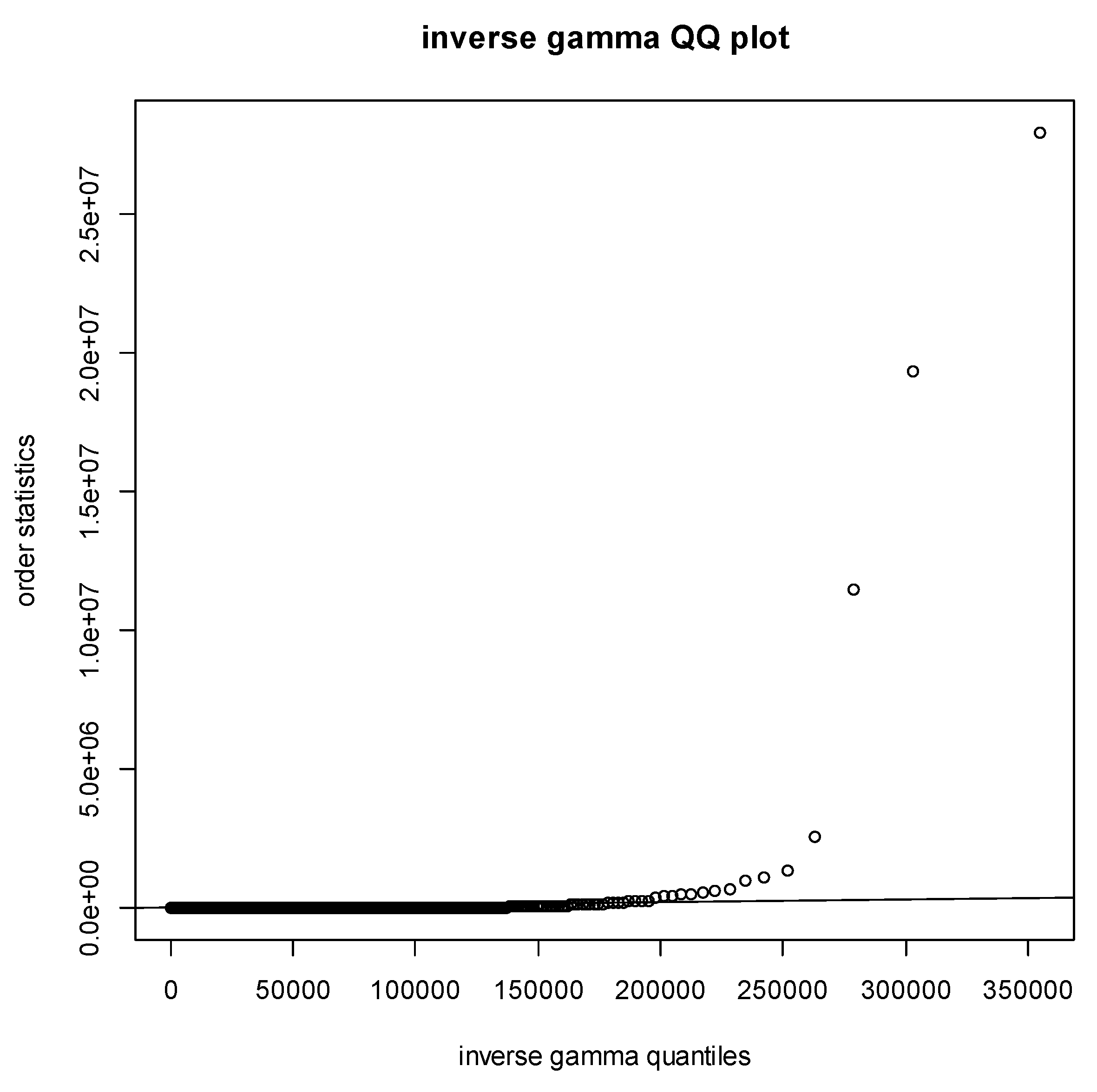
This formula is appealing, as it characterizes the Bayes estimate as the usual estimate pulled towards the prior mean. However, if we examine the actual volatilities of stocks, the inverse gamma does not appear to fit the volatility distribution well.
Figure 1 shows a quantile-quantile plot of the fitted gamma distribution. The non-linear appearance of the plot indicates the lack of fit of the inverse gamma.
4.2 An empirical Bayesian approach
To empirically apply a Bayesian approach we first calculated the annualized volatilities of the sample of 5,671 stocks, based on 30 trading days, beginning on November 17, 2009. A normal plot of the data revealed a right skewed distribution, suggesting a gamma distribution (rather than an inverse gamma) might fit this data well.
If the mean and variance of the volatilities are denoted by
and
var(v) respectively, then method of moments estimates of
r and
are
and
. We applied these formulas after removing the 10 most extreme values, obtaining
= 2.604585 and
= 0.01113419. The fit can be improved by a more refined estimation technique for the gamma parameters, namely maximum likelihood. This involves maximizing the log-likelihood:
as a function of
r and
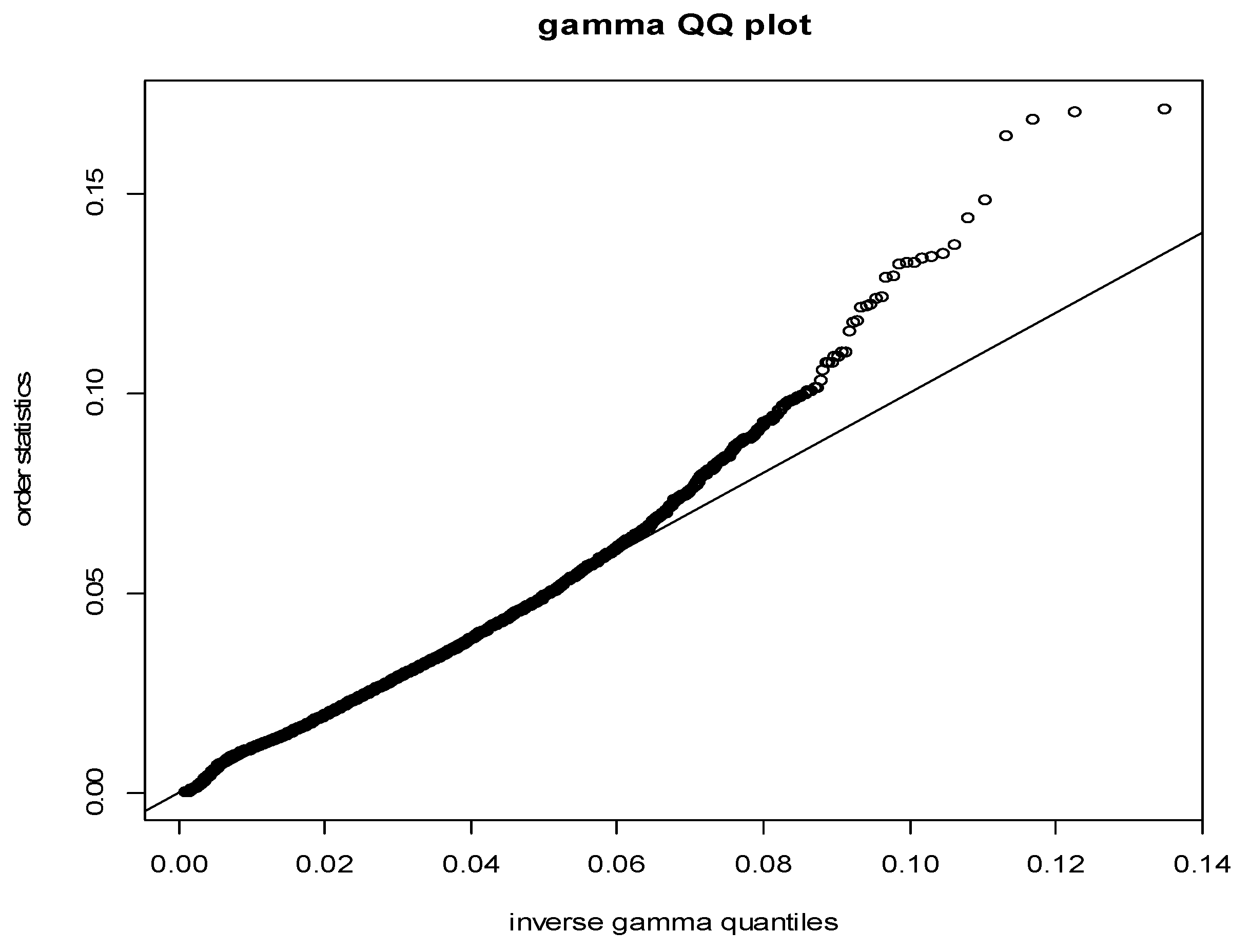
λ. The maximizing values (maximum likelihood estimates) are
= 3.051479 and
= 0.009503573 . The quantile plot with these estimates is shown in
Figure 2.
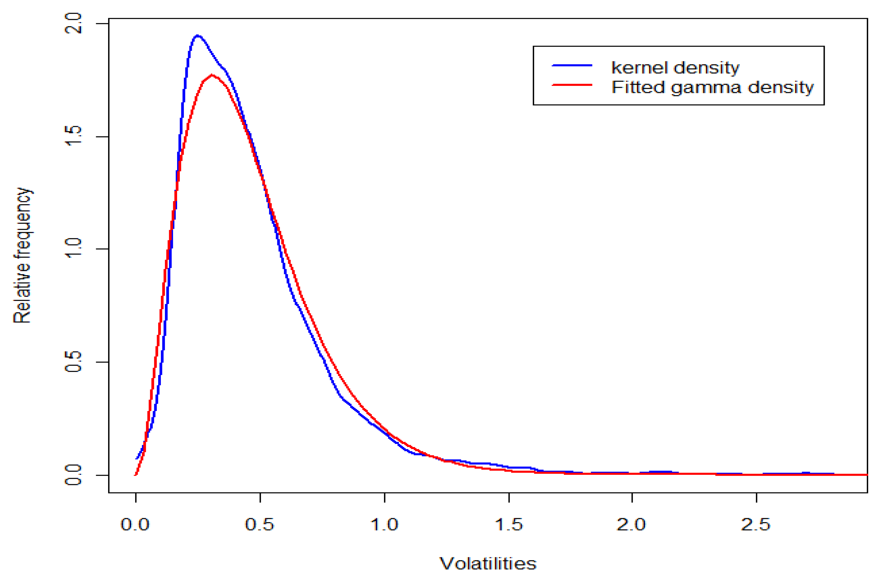
The plot represents a considerable improvement over the inverse-gamma fit, being much closer to the 45° line. A plot showing the fitted gamma density and a kernel density estimate of the volatilities is shown in
Figure 3. The figure shows a good degree of fit between the estimates.
To construct a Bayes estimator for the volatility of a particular stock, we can assume a prior distribution for the volatility coinciding with the gamma distribution above, and use the posterior mean as our estimate.
This results in the estimate
where
, and
V is the usual historic annualized volatility, given by:
based on n daily returns
x1,…, xn. In our calculations,
n was 30, corresponding to 30 day options.
The integrals in the estimate can be evaluated using standard numeric integration. Applying this to our November 17, 2009 data set with 275 implied and historical volatilities, and letting
,
and
be respectively the historic volatility, the implied volatility and the Bayes estimate, we get:
This indicates that the Bayes estimate provides about an 8% improvement.
There is a hint of a mixture in distribution in the volatilities, suggestive of two types of stock with differing volatilities, one more volatile than the other. To further improve the fit of the gamma distribution, we can fit a mixture of two gamma distributions to the volatility data, having density
where
f is given by (1), π is the mixing probability and
r1, r2, λ1 , λ 2 are the shape and scale parameters. The maximum likelihood estimates of these parameters are obtained using the EM algorithm (Dempster, Laird and Rubin, 1977), and a “Mixture Bayesian estimate” may be calculated by the formula:
where
The ability of these estimates (the historical volatility, and the three Bayesian estimates) to match the implied volatility is explored in the next section.
For each of the remaining periods (other than November 17, 2009) in the sample period between August 16, 2007 and November 17, 2009, we repeat the same procedure to recalculate the parameters under the gamma distribution to determine the three Bayesian volatility estimates.
4.3 Measurement of estimation error
For each of the three Bayesian estimates (those based on the conjugate prior, the gamma prior and the mixture prior respectively), we calculated a “Bayesian error” using the formula:
These errors were compared to the “historical error”
where the Bayesian volatility estimates are calculated in accordance with
Section 4.1 and
Section 4.2 above; the historical volatility is calculated in accordance with equation (5) and the IVolatilty is the implied volatility supplied by IVolatility.
5. EMPIRICAL RESULTS
The errors calculated above all have extremely right-skew distributions. Accordingly we compare these distributions using medians and the Wilcoxon test, rather than means and the t-test. For each 30-day time period, we made three comparisons by comparing the “historical error” to each of the three “Bayesian errors”. This was done separately for call and put options, although there is not much difference between them. A negative value indicates that the Bayesian error is greater.
For all time periods combined, the last lines of both Panels A and B of
Table 3 indicate that the Bayesian estimate using the conjugate prior does not perform better than the historical estimate. In Panel A of
Table 3 for call options, the difference in medians is small. The proportion of Bayesian errors using the conjugate prior that are less than the historical errors is 45%, so that the Bayesian estimate is significantly stochastically larger than the historical estimate (p=0.0007). For put options, Panel B of
Table 3, the situation is similar, with no significant difference between the Bayesian approach using the conjugate prior and historical methods.
For the Bayesian estimate using the gamma prior, the situation is reversed. For call options, Panel A of
Table 3, the difference in medians is now 0.00217, and the Bayesian estimate is significantly stochastically smaller, with 60% of the Bayesian errors being smaller (p<0.0001). The values for the put options, Panel B of
Table 3, are 0.00233 and 62% respectively. The results for the mixture prior for both call and put options are very similar to those for the gamma prior.
Table 3, Panels A and B, also show the results for each time period separately. The separate-period analyses further demonstrate the relatively poor performance of the conjugate Bayes estimate. For call options (
Table 3, Panel A), the median Bayesian error was less than the historic error in only 7 out of the 19 periods studied. Moreover, if we consider the proportion of stocks for which the Bayesian error was less than the historic error, we find that for only 7 out of 19 periods was this percentage greater than 50%. It seems that use of an inappropriate prior makes the Bayes estimate inferior to the historical volatility.
For call options the position is reversed when we consider the Gamma and mixture priors (
Table 3, Panel A). For both of these, the median Bayesian error was less than the historic error in 12 out of the 19 periods studied, with all 12 differences being significant at the 5% level on a Wilcoxon test. For the 7 periods where the historical method was better, 6 were significantly better for the Gamma priors and 5 were significantly better for the mixture priors.
Turning to the proportion of stocks for which the Bayesian error was less than the historic error, we find that for both the gamma and mixture priors, 13 out of the 19 periods studied had the percentage of stocks greater than 50%. Thus, there is a significant benefit in using the Bayesian estimate based on gamma prior over the historic estimate. There does not seem to be much advantage in using the mixture prior, mainly because the mixture is typically dominated by a single component.
For put options (
Table 3, Panel B), the situation is broadly similar. For the conjugate prior, 6 out of 19 periods have the median Bayesian error less than the historic, and only in 7 out of the 19 periods was the historical volatility percentage error greater than 50%. For the gamma prior, the results are 14/19 and 13/19 respectively, and for the mixture prior 14/19 and 14/19.
Overall the evidence suggests that the Bayesian volatility estimates based on the gamma and mixture priors provide a more accurate estimate of the implied volatility compared to the historical estimate of stock volatility.
In our Bayesian estimates, we have assumed that the 30-day sequences of log-returns are normally distributed. We tested the sequences for normality at each time point, and typically found about 23% failed the Shapiro-Wilk normality test. The detailed results are shown in
Table 4. This indicates that overall the estimates may be quite robust with respect to this assumption.
6. CONCLUSION
Options and derivative contracts are extensively traded on many exchanges and play an important role in the transfer of risk between hedgers and speculators. In pricing these instruments a key parameter input is an estimate of ex-ante volatility.
This paper investigates if Bayesian volatility estimates can provide a more accurate and reliable estimate of a stock’s implied volatility compared to a historical volatility estimate. The implied volatility of the stock is computed by IVolatility using traded options price, for at or near-the-money call and put options, on a sample of US stocks over the period between August 16, 2007 and November 17, 2009. Prior research suggests that implied volatility estimates from option prices provide a more accurate estimate of actual realised volatility compared to historical estimates.
Overall our results provide evidence that Bayesian volatility estimates based on the Gamma and mixture priors may provide a better estimate of implied option volatility than the historical volatility estimate. A more reliable estimate of ex-ante volatility compared to historical stock price volatility can be useful to price options on stocks that have no existing options traded and where an implied volatility estimate cannot be observed. For example, many US and offshore companies will have employee stock option schemes but no publicly traded options. However, these employee stock options must now be valued and expensed in accordance with US and international accounting standards. One drawback from our Bayesian approach is that the conjugate prior is not used, and therefore the posterior has to be solved numerically. However, since this involves integration with only one variable, it can still be solved easily without resorting to simulations.
Areas for future research include exploring the accuracy of our Bayesian estimates to the implied volatility of options with different terms to maturity other than 30 days and for call and put options that are well out or well in-the-money. Other avenues of research include comparing the relationship between Bayesian and historical volatility estimates, using pricing models other than the Black-Scholes or binomial options pricing model or comparing Bayesian forecasts to forecast volatility estimates based on exogenous variables such as GDP change, interest rates and other macro-economic indicators.


