Multiperiod Hedging using Futures: Mean Reversion and the Optimal Hedging Path

College of Management, Metropolitan State University,13th St & Harmon Place Minneapolis, MN 55403, USA
J. Risk Financial Manag. 2011, 4(1), 133-161; https://doi.org/10.3390/jrfm4010133
Published: 31 December 2011
Abstract
:This paper considers the multiperiod hedging decision in a framework of mean-reverting spot prices and unbiased futures markets. The task is to determine the optimal hedging path, i.e., the sequence of positions in futures contracts with the objective of minimizing the variance of an uncertain future cash flow. The model is used to illustrate both hedging using a matchedmaturity futures contract and hedging by rolling over a series of nearby futures contracts. In each case, the paper derives the conditions under which a single period (myopic) strategy would be optimal as opposed to a dynamic multiperiod strategy. The results suggest that greater the market power of the hedging entity, closer the optimal strategy is to a myopic hedge. The paper also highlights the difference in the optimal hedging path when hedging is based on matched-maturity as opposed to nearby contracts.
JEL Classification:
G32; G13ACKNOWLEDGEMENTS: I would like to thank Mike Sher and an anonymous referee for their comments on an earlier draft of this paper. Errors, of course, remain my own responsibility.
1. INTRODUCTION
Consider the hedging problem of a firm facing an uncertain future cash flow at a certain future time, T. The uncertain future cash flow (referred to as the hedged item) may arise from a fixed cash or spot position or, more generally, from revenues/costs/profits in a certain future period referred to as the terminal or target period. The hedging horizon (i.e. the time between now and the future terminal date T) is broken up into a series of discrete intervals, and the decisionmaker's task is to choose futures positions for each period so as to minimize the variance of the future cash flow. For example, the model may be applied to a commodity trader hedging a forward commitment or a firm hedging future input costs.
In a classic, widely-cited study, Howard and D’Antonio (1991), henceforth referred to as HD, derived the optimal hedging strategy in a framework of mean-reverting spot returns and unbiased futures markets. Their main result is that the optimal hedging strategy depends crucially on the rate of mean reversion of the spot process (i.e., the price process of the hedged item, also referred to as the “hedged process”). The current study extends the analysis by explicitly allowing for mean reversion in the price process of the underlying of the futures contract as well (referred to as the “hedging process”). In this extended framework, the HD model may be viewed as a special case in which hedging is carried out by rolling over a series of nearby contracts (“stack and roll” hedging, or just “stack” hedging). The current study considers hedging based on matched-maturity futures contracts (i.e., contracts maturing at the same time as the occurrence of the cash flow being hedged) as well as hedging based on nearby futures contracts. It is seen that if hedging is based on matched-maturity contracts, the optimal hedging strategy depends not so much on the absolute mean reversion rate of the hedged process (as in the case of hedging using nearby contracts), but rather on the relative mean reversion rates of the hedged and hedging processes.
The main contributions of the current paper are as follows. A simple, but empirically relevant setting of mean-reverting prices is used to illustrate matched-maturity hedging and compare it to stack hedging. However, the focus is not on determining if one is better than the other. Rather, the objective is to determine the optimal hedging path in each case. Possible multiperiod hedging paths can be grouped into three categories: (i) a static multiperiod hedge, wherein the hedge position is taken at the start of the hedging horizon and then kept unchanged until the terminal period, (ii) a myopic or single-period hedge, wherein the hedge position is initiated only at the start of the terminal period, and (iii) a dynamic hedge, wherein hedging is initiated at the start of the hedging horizon and updated each period. The focus is on the conditions under which each of these categories is optimal. It is shown that, in general, the optimal hedging path or pattern can be very different depending on whether hedging is carried out using matched-maturity or nearby futures contracts. The exception to this is when futures prices follow a random walk.
In addition to HD, another study to which the current paper has a strong relation is Myers and Hanson (1996), hereafter referred to as MH. Their paper deals with the same problem of hedging a fixed cash position in the presence of basis risk. They show that provided futures prices evolve as a martingale, it is possible to derive an optimal dynamic hedging strategy that is independent of risk preferences under fairly general assumptions about the relationship between spot and futures prices. As will be elaborated upon later, the current paper may be viewed as a special case of the MH model. As a result, the variance-minimizing hedge derived in the current study is also the expected-utility maximizing hedge.
The next section contains a review of the literature, the following section develops the model and discusses implications and the final section concludes with a brief summary of the main results.
2, LITERATURE REVIEW
Several studies have examined the hedging behavior of firms facing price or exchange rate uncertainty in input/output markets. A seminal study by Johnson (1960) analyzed the hedging decision as an optimal portfolio problem and derived the minimum variance hedge ratio. While Sandmo (1971) showed that a firm’s output decision would be affected by price uncertainty, Danthine (1978) and Holthausen (1979) showed that in the presence of a forward market to hedge away this uncertainty, the output decision would be independent of this risk and the firm’s risk preferences. Extensions and refinements were made by Losq (1982), Fishelson (1984) and Zilcha and Broll (1992) among many others. De Meza and von Ungern Sternberg (1980) derived the result that a monopolistic firm is more likely to hedge input risk than a competitive firm as volatile input prices will have a bigger impact on the profits of the former. Koppenhaver and Swidler (1996) investigated how the degree of market power enjoyed by a firm in the output market affects the extent to which the firm will hedge its input price risk. They concluded that lower the market power of the firm, more the importance of hedging. These studies are set in a single-period framework and focus on the relationship between hedging strategies and output decisions in the context of specific market structures. The decision-maker’s objective is typically assumed to be maximizing expected utility or minimizing the variance of end-of-period wealth. Examples of discrete-time, multi-period models investigating the dependency between the production and the hedging decision include Zilcha and Eldor (1991) and Donoso (1995). Among other things, these studies show that the firm will overhedge when current shocks can adversely affect future cash flows.
Another set of studies focuses on the optimal hedging strategy for a trader or producer who will liquidate a non-tradable cash position at a certain future time, T. The hedging horizon (i.e. the time between now and the future terminal date T) is broken up into a series of discrete intervals, and the decision-maker's task is to choose futures positions for each period so as to maximize expected utility of end-of-period wealth or minimize the variance of end-of-horizon wealth/cash flow. Some of these models ignore basis risk (Anderson and Danthine, 1983) and others assume negative exponential utility with a joint normal distribution for cash and futures price changes (Karp, 1987, Martinez and Zering, 1992, and Vukina and Anderson, 1993). A few studies have tackled the optimal dynamic hedging problem in a discrete-time setting without making restrictive assumptions either about risk preferences or the distribution of prices. Notable studies of this kind include HD and MH, mentioned earlier in the introduction and discussed in more detail in the next section. The interested reader is referred to Low, Muthuswamy, Sakar and Terry (2002) for a more extensive review.
While much of the discrete-time literature is based on expected utility maximization or variance minimization, some studies have explored alternative hedging objectives such as regret minimization and approaches based on the mean-extended Gini coefficient and the semivariance. Chen, Lee and Shrestha (2003) provide a fairly comprehensive review of these alternative theoretical approaches to hedging. Yet another branch is concerned with empirical testing of alternative estimation models and techniques, such as Ordinary Least Squares Regression, Cointegration and Error Correction models, Generalized Autoregressive Conditional Heteroscedasticity (GARCH) models and stochastic volatility models. The interested reader is referred to Lien and Tse (2002) for an excellent review of these various econometric approaches and estimation methods. Some noteworthy recent empirical studies include Hung and Lee (2007), who focus on minimizing down-side risk in the presence of volatility clustering and price jumps, Power and Vedenov (2008), who estimate a copula-GARCH model, Huang, Pan and Lo (2010), who compare a duration-dependent Markov-switching vector autoregression approach with GARCH models, Chan (2010), who employs a GARCH model that is modified to allow for jumps, Cao, Harris and Shen (2010), who use a non-parametric approach to estimate hedge ratios designed to minimize Value-at-Risk, and Chen and Tsay (2011), who use a novel approach to estimate a Markov regime-switching, Autoregressive Moving Average model.
There is also a vast literature that investigates optimal hedging in continuous-time. Early classics include Breeden (1984), Adler and Detemple (1988), Duffie and Jackson (1990) and Duffie and Richardson (1991). Breeden (1984) provides the dynamic optimal hedging strategy in terms of the value function for an agent maximizing expected utility of intertemporal consumption, while Adler and Detemple (1988) consider the problem of an agent hedging a nontraded spot position and maximizing logarithmic utility of terminal wealth, and derive an explicit, analytical solution for the case in which markets are complete. Duffie and Jackson (1990) and Duffie and Richardson (1991) consider the optimal hedging problem in a setting in which prices follow Geometric Brownian Motion (GBM) and derive explicit solutions for various mean-variance hedging objectives. Among recent studies, Basak and Chabakauri (2008) provide a good summary of this literature and also provide explicit, tractable solutions to the dynamic hedging problem of a non-tradable asset. Ankirchner and Heyne (2012) solve the problem for the case of stochastic correlation between the process being hedged and the hedging instrument, and Ankirchner, Dimitroff, Heyne and Pigorsch (2012), the case in which the (log) spread between the hedged and hedging processes is stationary (which is not the case when the two processes follow GBM).
As is apparent from the above, there is an extensive literature on dynamic hedging using futures. Below are described some recent studies (other than HD and MH) to which the current study is closely related and a summary of how the current study complements these prior studies.
Hilliard (1999) uses a continuous time setting in which prices follow Geometric Brownian motion to derive optimal hedging results using a “stack and roll” strategy. Neuberger (1999) studies a similar problem, but with a focus on “strip” hedges (i.e., hedging using futures contracts of multiple maturities). The model is based on assumptions about the cross-sectional character of futures prices of different maturities rather than assumptions about their time-series dynamics. In both these studies, the future commitment that is being hedged is far enough in the future so that hedging using a matched-maturity futures contract is either not possible or not economical. In contrast, the current study explicitly considers hedging based on matched-maturity contracts and is set in a different setting of discrete-time, autoregressive prices.
Another strand of research extends from a noteworthy study by Lien and Luo (1993) in which they derive the optimal multiperiod hedging strategy and apply it in a setting of cointegrated spot and futures prices. Their empirical results clearly show the superiority of multiperiod hedging over a myopic (single-period) strategy. Building on this work, Low et al (2002) study multiperiod hedging in a setting in which the futures price follows a cost of carry model. This allows them to capture the effect of the maturity of the futures contract on the spot-futures basis. Their empirical tests show that their “dynamic cost-of-carry hedge” outperforms other strategies such as the conventional (myopic) hedge, the cointegrated price hedge of Lien and Luo (1993), and the GARCH hedge of Kroner and Sultan (1993), although a static, cost-of-carry hedge is found to perform slightly better. Lien and Shaffer (2002) use a three period setting to compare the effectiveness of “strip” hedging with “stack” hedging in managing the risk of a forward commitment. They use a Vector Autoregressive framework to model spot and futures prices and show that “strip” hedging outperforms “stack” hedging especially when forward prices are subject to multiple risk factors. The current study is similar to these studies in that it investigates the same multiperiod hedging problem. However, it differs from these studies in some important respects. Firstly, the current study is set in a framework of mean-reverting rather than non-stationary prices. It is, of course, true that price processes of many assets – especially financial assets - have been determined to be non-stationary, as noted in the above studies. However, as concluded by Bessembinder, Coughenour, Smoller, and Seguin (1995) and noted in Schwartz (1997), a mean reverting process is a good description of the price dynamics of many commodities. Secondly, the main focus of the current study is different. Unlike these prior studies, the current paper does not attempt to assess the empirical performance of alternative hedging approaches. Instead, using a simple, but empirically useful framework, the paper makes clear (i) the connection between the relative rates of mean reversion of hedged and hedging processes on the one hand and the optimal multiperiod hedging strategy on the other, (ii) the conditions under which a single period (myopic) strategy, a static multiperiod strategy and a dynamic multiperiod strategy would each be optimal in this framework, and (iii) the difference in the optimal hedging path when hedging is based on matched-maturity as opposed to nearby contracts.
3. MODEL
Suppose that the hedger has a fixed cash position, x. The hedger will liquidate this position at terminal time T and faces the problem that the price of the hedged item as of time T is uncertain. Suppose that the price process of the hedged item (the “hedged process”) is given by:
Above, pt is the value of the process in period t. If ϕ = 1, then pt follows a random walk. If ϕ is strictly between 0 and 1, µ is the long run mean of pt and (1-φ) is the speed of adjustment of pt to the long run mean. If ϕ = 0, then pt is independently and identically distributed (i.i.d.) each period. Thus, higher the value of ϕ, lower is the degree of mean reversion. Similar to the model in HD, it is assumed that ut is i.i.d. with variance . The process for pt may be equivalently expressed as
Similarly, let yt denote the price process of the underlying of the futures contract (the “hedging process”).
Above, yt is the value of the process in period t, κ is the long run mean, and (1-θ) is the rate of mean-reversion. ξt is assumed to be i.i.d. with variance . Further, ut and ξt are assumed to be contemporaneously correlated with covariance σuξ, but all noncontemporaneous covariances are assumed to be zero.
pt − pt−1 = (1 − ϕ)(μ − pt −1) + ut
pt = (1 − ϕ)μ + ϕpt−1 + ut
yt − yt−1 = (1 − θ)(κ − yt−1) + ξt
Let denote the futures price in period T-k of the contract that matures in period T. Similar to HD and MH, the current study assumes unbiased futures prices.1 This assumption can be stated as follows:
![Jrfm 04 00133 i001]() where Et is the expectations operator conditional on information available in period t.
where Et is the expectations operator conditional on information available in period t.

Take the hedger’s objective to be to minimize the variance of the cash flow at time T. (As discussed subsequently, the variance-minimizing hedge is also the strategy that maximizes the expected utility for any increasing, concave utility function.)
3.1 Hedging with Matched-Maturity contracts
The following assumes that the hedger uses matched-maturity futures contracts (i.e., contracts maturing at time T). The case of hedging with nearby futures contracts is considered later. Suppose that the earliest the hedger may initiate hedging is N periods prior to T. (This may be due to non-availability or lack of liquidity of longer-term futures contracts.) For 1 ≤ k ≤ N, let bT-k denote the hedge ratio (i.e., futures position per unit of the spot position).
The post-hedge cash flow in period T is given by
![Jrfm 04 00133 i002]() Above, it is assumed that futures positions are marked-to-market each period, and r is the constant, periodical interest rate used to compound intermediate, mark-to-market cash flows.
Above, it is assumed that futures positions are marked-to-market each period, and r is the constant, periodical interest rate used to compound intermediate, mark-to-market cash flows.

As in HD, the optimal hedge ratios can now be derived by working backwards from the terminal period. As derived in Appendix A, the optimal hedge ratio at time T-k is given by
![Jrfm 04 00133 i003]()

The optimal hedging strategy derived above has several interesting features and implications. First, note that one period before the terminal date, the hedge ratio reduces to the standard single-period optimal hedge ratio, σuξ/, derived by Ederington (1979). Second, the hedging strategy derived above is dynamically optimal. Each period's hedge position is chosen after taking into account optimal hedging behavior in the future. Third, the model can be used to not only hedge a long or short cash position, but can also be readily adapted to hedging a future cash flow (such as a future period’s revenues or costs or operating cash flows) by letting the hedged process, p, denote the relevant cash flow, setting the non-stochastic cash position x equal to unity, and interpreting bt as the futures position rather than the hedge ratio. Fourth, the model can be (obviously) used for hedging (either a fixed cash position or a future cash flow) not just on a one-time basis, but on an on-going basis. The optimal hedging strategy can then be viewed not just as minimizing the variance of a single future cash flow, but as minimizing the volatility of the time series of cash flows (provided the spot price process does not follow a random walk). For example, the model can be applied to a firm trying to minimize the volatility of its monthly foreign currency revenues (input costs) by hedging each month’s foreign currency receipts (consumption) over “N” prior months. Fifth, the model can be readily adapted to hedging using forward contracts. As shown in part B of the Appendix, the optimal, cumulative hedge ratio at time T-k for hedging using forward contracts is given by
![Jrfm 04 00133 i004]() Sixth, this model can be shown to be a special case of the model developed in Myers and Hanson (1996), referred to as MH. In this paper, they show that provided futures prices evolve as a martingale, it is possible to derive an optimal dynamic hedging strategy that is independent of risk preferences under fairly general assumptions about the relationship between spot and futures prices. All they require of the utility function is that it should be increasing and strictly concave. As shown in part C of the Appendix, the assumptions in the current model satisfy the conditions laid out in the MH framework. Consequently, the optimal hedging strategy derived in this study not only minimizes the variance of the net cash flow on the terminal date, but also maximizes the terminal date expected utility. This is related to the results in Lence (1995) and Rao (2000) derived in a single-period setting.
Sixth, this model can be shown to be a special case of the model developed in Myers and Hanson (1996), referred to as MH. In this paper, they show that provided futures prices evolve as a martingale, it is possible to derive an optimal dynamic hedging strategy that is independent of risk preferences under fairly general assumptions about the relationship between spot and futures prices. All they require of the utility function is that it should be increasing and strictly concave. As shown in part C of the Appendix, the assumptions in the current model satisfy the conditions laid out in the MH framework. Consequently, the optimal hedging strategy derived in this study not only minimizes the variance of the net cash flow on the terminal date, but also maximizes the terminal date expected utility. This is related to the results in Lence (1995) and Rao (2000) derived in a single-period setting.

The points mentioned above are explicit or implicit in HD and/or in MH. The main point of the current paper is the following, which is a consequence of the additional structure imposed in the current study. As evident from (6), the optimal hedging strategy depends in an important manner on the relative magnitudes of ϕ and θ, which, as discussed below, may be influenced by the extent of market power enjoyed by the firm. The case ϕ = θ reflects the situation in which both the hedged process and the hedging process mean-revert with the same speed. This is likely to occur when the hedged and hedging processes are either the same or closely related (such as jet fuel and crude oil). If ϕ < θ, the hedged process mean-reverts at a faster rate than the underlying of the futures contract. (Recall that the rate of mean reversion is one minus the autoregressive coefficient.) This is likely to be an empirically important case. For example, consider an airline hedging its operating cash flows against jet fuel price fluctuations using oil futures. In this case, the hedged process is the operating cash flow and the hedging process is oil price. Suppose that the firm is faced with an adverse shock, such as an increase in oil prices. If the firm has some degree of market power, it may be able to raise the price of its product at least partially and with a lag even if not immediately. As a result, its cash flows may recover (or revert to previous levels) quicker than the price of oil goes back down. In general, greater the pricing power of the firm, the better the firm can respond to adverse shocks, and therefore faster will be the mean reversion of its operating cash flows and hence smaller the ratio of ϕ to θ. Lastly, if θ < ϕ, the hedged series mean-reverts slower than the underlying of the forward contract. This would, for example, reflect a situation in which operating cash flows take more time to return to pre-shock levels than the hedging process. Such cases are probably less common in the real world.
INSERT TABLE 1 AND GRAPH 1 ABOUT HERE
Table 1 illustrates how the optimal hedging strategy changes with the ratio of ϕ to θ. For ease of exposition, σuξ/ (the ratio of the covariance between the shocks affecting the hedged and hedging processes to the variance of the hedged process) is set equal to unity. For simplicity, the interest rate, r, is set equal to zero. Therefore, the results in the table may be interpreted as relating to hedging using forward contracts rather than futures. Thus, the table contains optimal, cumulative hedge positions in forward contracts for a few selected values of the ratio of ϕ to θ. It is assumed in the calculations that the number of prior periods over which hedging is possible is twelve (i.e., N = 12).
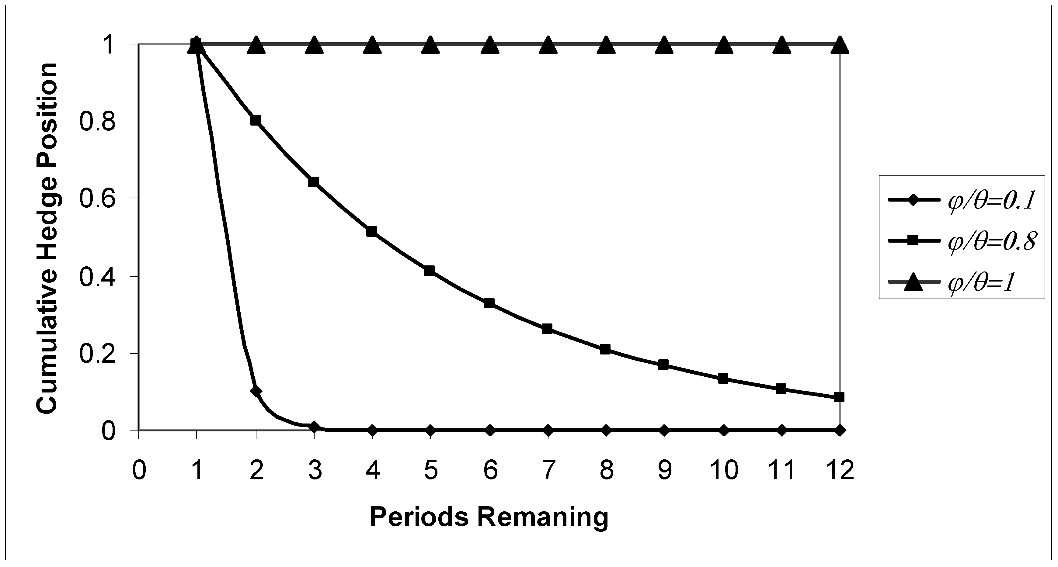
For convenience, define a “back-loaded” strategy as one in which substantial hedging positions are taken only in the period(s) just prior to the terminal date and a “front-loaded” strategy as one in which substantial hedging positions are taken well in advance of the terminal date. Now, consider the case, ϕ/θ=1, in which both the hedged and hedging processes mean-revert at the same rate. In this case, the optimal strategy is seen to be a front-loaded strategy. In fact, the optimal strategy is essentially a static, multiperiod hedge – i.e., to undertake a complete hedge as far ahead as possible and retain this position until the terminal date. However, if the ratio is strictly between zero and one, then the optimal strategy is to spread the hedging activity over multiple periods. For example, if the ratio is 0.8, as shown in Table 1, the hedger should enter into a partial hedge to the extent of 8.59% of the optimal single period hedge twelve periods prior to the terminal date. The hedger should gradually increase the hedge position each subsequent period such that it is 64% three periods prior to the terminal date and, of course, 100% one period prior. In general, both Table 1 and Graph 1 illustrate that smaller the ratio of ϕ to θ, smaller should be the size of the initial position with most of the hedging concentrated in the last few periods prior to the terminal date. Closer the ratio is to zero, more back-loaded the strategy should be. If the hedged process mean-reverts at a considerably faster rate than the hedging process (ϕ << θ) perhaps as a consequence of the firm’s market power, distant shocks have a relatively small impact on the firm and only short-term shocks (i.e., shocks close to the terminal date) need to be hedged against. Indeed, if the ratio is zero, then a single period (myopic) hedging strategy (of entering into a hedge only at the start of the terminal period) would be perfectly appropriate. On the other hand, larger the ratio of ϕ to θ, larger should be the hedging positions taken in earlier periods. In fact, if it is the hedged process that mean-reverts slower (ϕ > θ), then the optimal hedging strategy is to overhedge in the initial period, and then reverse out the excess position gradually as the terminal date draws near. This is illustrated in the last column of Table 1.
3.2 Hedging using nearby contracts (stack hedging)
Now consider how the optimal hedging strategy will be different if hedging is carried out by rolling over a series of nearby contracts.2 For simplicity, it is assumed that futures contracts are available for all expiration dates leading up to the terminal date.
As shown in part D of the Appendix, the optimal hedging strategy is now given by
![Jrfm 04 00133 i005]() As may be seen, the autoregressive coefficient of the hedging process, θ, plays no role. The result above is similar to the one derived by HD. (The result in HD is slightly different as in their model, the hedger is hedging not just one future cash flow but several. This paper considers the simpler problem of hedging just one future cash flow in order to simplify the exposition and ensure that a key point of the paper, namely the difference between hedging using nearby contracts and hedging using matched-maturity contracts, is made as clearly as possible.) If the autoregressive coefficient of the hedged process, ϕ, is close to zero, then the optimal hedge ratio in all prior periods from T-2 through T-N would be close to zero; and the optimal hedge ratio one period prior to the terminal period (i.e., as of T-1) would, of course, equal the standard single period optimal hedge. Thus, a single period (myopic) approach to hedging would be appropriate only in the case in which the hedged process is independently and identically distributed. Conversely, a front-loaded strategy of taking large hedging positions several periods prior to the terminal date is optimal only if ϕ is close to unity – i.e., if the rate of mean reversion of the hedged process is so slow that the process is close to being a random walk. Note that the values in Table 1 can be used to illustrate hedging using nearby contracts as well, with the difference that each column of Table 1 should be taken to represent a particular value of ϕ rather than the ratio of ϕ to θ.
As may be seen, the autoregressive coefficient of the hedging process, θ, plays no role. The result above is similar to the one derived by HD. (The result in HD is slightly different as in their model, the hedger is hedging not just one future cash flow but several. This paper considers the simpler problem of hedging just one future cash flow in order to simplify the exposition and ensure that a key point of the paper, namely the difference between hedging using nearby contracts and hedging using matched-maturity contracts, is made as clearly as possible.) If the autoregressive coefficient of the hedged process, ϕ, is close to zero, then the optimal hedge ratio in all prior periods from T-2 through T-N would be close to zero; and the optimal hedge ratio one period prior to the terminal period (i.e., as of T-1) would, of course, equal the standard single period optimal hedge. Thus, a single period (myopic) approach to hedging would be appropriate only in the case in which the hedged process is independently and identically distributed. Conversely, a front-loaded strategy of taking large hedging positions several periods prior to the terminal date is optimal only if ϕ is close to unity – i.e., if the rate of mean reversion of the hedged process is so slow that the process is close to being a random walk. Note that the values in Table 1 can be used to illustrate hedging using nearby contracts as well, with the difference that each column of Table 1 should be taken to represent a particular value of ϕ rather than the ratio of ϕ to θ.

3.3 Hedging using matched-maturity contracts v/s nearby contracts
From (3) and (4),
![Jrfm 04 00133 i006]()
![Jrfm 04 00133 i007]() Thus, futures contracts of all maturities are perfectly correlated under the assumptions of our model, which is, of course, an immediate consequence of the fact that in this model, the entire term structure of futures price is driven by a single risk factor. Therefore, both hedging strategies – based on matched-maturity contracts and rolling over nearby contracts – will be equally effective (in the sense that both strategies will result in the same variance of terminal cash flow). However, as mentioned earlier, it is not the comparative effectiveness of these two strategies that is the focus of this paper, but rather the difference in the optimal hedging path and the conditions that determine the path in each of these cases.
Thus, futures contracts of all maturities are perfectly correlated under the assumptions of our model, which is, of course, an immediate consequence of the fact that in this model, the entire term structure of futures price is driven by a single risk factor. Therefore, both hedging strategies – based on matched-maturity contracts and rolling over nearby contracts – will be equally effective (in the sense that both strategies will result in the same variance of terminal cash flow). However, as mentioned earlier, it is not the comparative effectiveness of these two strategies that is the focus of this paper, but rather the difference in the optimal hedging path and the conditions that determine the path in each of these cases.


INSERT TABLE 2 ABOUT HERE
The main differences between the two cases (hedging with matched-maturity v/s nearby futures) are summarized in Table 2. It is clear that the optimal hedging strategy can be very different between hedging based on matched-maturity contracts and hedging based on nearby contracts. For example, if ϕ = θ < 1, then if hedging is based on matched-maturity contracts, the optimal strategy is a static multiperiod hedge, while if hedging is carried out by rolling over nearby futures, then the optimal strategy is either front-loaded or back-loaded depending on how close ϕ is to zero. However, it is also apparent that if the price process of the underlying of the futures contract follows a random walk (i.e., if θ = 1), then the optimal hedging path is the same regardless of whether hedging is based on matched-maturity or nearby contracts.
It may be noted that in the case of both hedging with nearby contracts and hedging with matched-maturity contracts, if the model is applied to hedging on an ongoing or rolling basis, the optimal hedging strategy may entail taking hedging positions that exceed the quantity required to hedge just a single future period’s cash flow. For example, suppose that the ratio of autoregression coefficients is 0.8, and consider a firm using matched-maturity forwards to hedge monthly cash flows on a rolling twelve-month basis. For this firm, the quantity of forward contracts held at any point in time would be 465% of the quantity required to hedge a single period’s cash flow. (4.65 is the sum of the hedge ratios in the appropriate column of Table 1).
4. CONCLUSION
This study examines the multiperiod hedging decision relating to a stochastic future cash flow in a setting of mean-reverting price processes and unbiased futures markets. It is seen that the optimal multiperiod hedging strategy depends in an important way on whether hedging is carried out using nearby or matched-maturity contracts. The question of interest is the hedging path – whether it is optimal to undertake a back-loaded strategy (in which substantial hedge positions are taken only in the period(s) just prior to the terminal date) or a front-loaded strategy (in which substantial hedge positions are taken well in advance of the terminal date). In the case of hedging with nearby contracts, the answer depends on the rate of mean reversion of the hedged process. However, in the case of hedging with matched-maturity contracts, the optimal strategy depends crucially on the relative rates of mean reversion of the hedged and hedging processes. If both processes mean-revert at roughly the same rate, then the optimal strategy is a front-loaded path. However, higher the rate of mean reversion of the hedged process relative to that of the futures contract’s underlying, the greater the appropriateness of a back-loaded (myopic or single period) strategy.
FOOTNOTES:
- 1.The issue of whether forward/futures prices are unbiased remains controversial. See Deaves and Krinsky (1995) for a good summary of early studies of this issue. Chinn and Coibion (2010) is a more recent study that also contains a good review of this topic and their findings appear to support this hypothesis for a range of commodities, especially energy related ones such as crude oil, heating oil, natural gas, and gasoline. They also find that even for non-energy commodities, “with almost no exceptions, we cannot reject the null of unbiasedness for the last five years of our sample, despite numerous departures from the null in the early and middle periods of our sample.” In any case, making any other assumption in its place would only serve to obscure the arguments of this paper.
- 2The term “nearby” contract is being used to mean a contract that will mature in the very next period. This is, of course, an assumption made primarily for convenience. However, it may be a close-enough approximation for practical purposes.
APPENDIX
A Hedging with matched-maturity futures contracts
As in the main body of the paper, N stands for the number of periods from today to terminal time T. For 1 ≤ k ≤ N, bT-k denotes the hedge ratio (i.e., futures position per unit of the spot position taken at time T-k in order to hedge time T cash flows).
By repeated substitution, for n ≥ 1, the price process for the hedged item, equation (2), can be expressed as:
![Jrfm 04 00133 i008]() Similarly, the price process of the futures contract’s underlying, the hedging process in equation (3) can be expressed as:
Similarly, the price process of the futures contract’s underlying, the hedging process in equation (3) can be expressed as:
![Jrfm 04 00133 i009]() Using the unbiased futures price assumption, it is seen that, for 1 ≤ k ≤ N
Using the unbiased futures price assumption, it is seen that, for 1 ≤ k ≤ N
![Jrfm 04 00133 i010]()
![Jrfm 04 00133 i011]() Note that futures prices are unbiased, but do not follow a random walk.
Note that futures prices are unbiased, but do not follow a random walk.


As mentioned in the main body of the paper, the post-hedge cash flow in period T is given by
![Jrfm 04 00133 i012]() Above, the non-stochastic spot position has been normalized to unity for convenience. As in HD, the optimal hedge ratios can now be derived by working backwards from the terminal period.
Above, the non-stochastic spot position has been normalized to unity for convenience. As in HD, the optimal hedge ratios can now be derived by working backwards from the terminal period.

With one period to go (that is, as of time T-1),
![Jrfm 04 00133 i013]() Using (A3) and (2), this can be expanded as follows:
Using (A3) and (2), this can be expanded as follows:
![Jrfm 04 00133 i014]() The variance of CT (focusing only on the error terms) is given by
The variance of CT (focusing only on the error terms) is given by
![Jrfm 04 00133 i015]() Differentiating with respect to bT-1, and setting the derivative equal to zero yields
Differentiating with respect to bT-1, and setting the derivative equal to zero yields
![Jrfm 04 00133 i016]() The second derivative is 2, which is obviously positive, and it is thus clear that the second order condition for a minimum is satisfied.
The second derivative is 2, which is obviously positive, and it is thus clear that the second order condition for a minimum is satisfied.


Next, with two periods to go,
![Jrfm 04 00133 i017]() Using (A1) and (A4),
Using (A1) and (A4),
![Jrfm 04 00133 i018]() The variance of CT is given by
The variance of CT is given by
![Jrfm 04 00133 i019]() Noting that optimal bT-1 is a known constant and using the first order condition gives the result
Noting that optimal bT-1 is a known constant and using the first order condition gives the result
![Jrfm 04 00133 i020]() The second derivative is
The second derivative is
![Jrfm 04 00133 i021]() This is clearly positive, and thus the second order condition for a minimum is satisfied. In general, k periods prior to T, the variance of the cash flow in period T is given by
This is clearly positive, and thus the second order condition for a minimum is satisfied. In general, k periods prior to T, the variance of the cash flow in period T is given by
![Jrfm 04 00133 i022]()


In any prior period, the optimal futures positions for subsequent periods are known constants. Using the first order condition for the optimal hedge ratio at time T-k, we arrive at the optimal hedge ratio, which is equation (6) in the main body of the paper:
![Jrfm 04 00133 i023]() The second derivative is
The second derivative is
![Jrfm 04 00133 i024]() This is clearly positive and thus the second order condition for a minimum is satisfied.
This is clearly positive and thus the second order condition for a minimum is satisfied.


B Hedging with matched-maturity forward contracts
The derivation of the optimal hedge ratio is very similar to that above, and is being provided mainly for completeness. Let denote the forward price in period T-k of the forward contract that matures in period T. As per the assumption of unbiased forward prices:
![Jrfm 04 00133 i025]() where Et is the expectation operator conditional on information available in period t.
where Et is the expectation operator conditional on information available in period t.

The post-hedge cash flow in period T is given by
![Jrfm 04 00133 i026]() Normalizing the cash position x to unity for convenience, using equations (A1) and (A3), and collecting terms,
Normalizing the cash position x to unity for convenience, using equations (A1) and (A3), and collecting terms,
![Jrfm 04 00133 i027]() For 1 ≤ n ≤ N, the variance of the cash flow in period T is given by (focusing on the error terms)
For 1 ≤ n ≤ N, the variance of the cash flow in period T is given by (focusing on the error terms)
![Jrfm 04 00133 i028]() Above, is the variance of the error term, u; is the variance of the error term, ξ; and σuξ is the covariance of these error terms.
Above, is the variance of the error term, u; is the variance of the error term, ξ; and σuξ is the covariance of these error terms.


The optimal hedge ratios can be derived by working backwards. Let hT-k denote the cumulative hedge ratio (cumulative futures position per unit of spot position) as of time T-k.
![Jrfm 04 00133 i029]() With one period to go (that is, as of time T-1),
With one period to go (that is, as of time T-1),
![Jrfm 04 00133 i030]() This can be expanded as follows:
This can be expanded as follows:
![Jrfm 04 00133 i031]() and the variance of CT is given by (taking n to be 1 in equation B4)
and the variance of CT is given by (taking n to be 1 in equation B4)
![Jrfm 04 00133 i032]() Differentiating with respect to hT-1, and setting the derivative equal to zero gives the result that
Differentiating with respect to hT-1, and setting the derivative equal to zero gives the result that
![Jrfm 04 00133 i033]() The second derivative is 2, and it is thus clear that the second order condition is satisfied.
The second derivative is 2, and it is thus clear that the second order condition is satisfied.


Next, with two periods to go,
![Jrfm 04 00133 i034]() This can be rewritten as
This can be rewritten as
![Jrfm 04 00133 i035]() And the variance of CT is given by
And the variance of CT is given by
![Jrfm 04 00133 i036]() The first order condition for optimal hT-2 is
The first order condition for optimal hT-2 is
![Jrfm 04 00133 i037]() Note that bT-1 is a known constant given by
Note that bT-1 is a known constant given by
![Jrfm 04 00133 i038]() Using the first order condition gives the result
Using the first order condition gives the result
![Jrfm 04 00133 i039]() The second derivative is seen to be
The second derivative is seen to be
![Jrfm 04 00133 i040]() This is clearly positive, and thus the second order condition for a minimum is satisfied.
This is clearly positive, and thus the second order condition for a minimum is satisfied.


In any prior period, the optimal forward positions for subsequent periods are known constants. Proceeding along the same lines as above, we arrive at equation (7) in the paper:
![Jrfm 04 00133 i041]()

C The Myers and Hanson (1996) framework
As in the current paper, the Myers and Hanson (MH) model considers a hedger with a nonstochastic cash position, x, which will be liquidated on a certain future terminal date, T. The hedger’s problem relates to the stochastic cash price at that time, pT. Each period, the hedger chooses a hedge ratio, bt, and enters into a futures position, bt x, at the prevailing futures price, ft. Futures positions are marked to market at the end of each period. The hedger’s wealth at the end of each period is given by:
![Jrfm 04 00133 i042]()
![Jrfm 04 00133 i043]() Above, r is the constant interest rate per period, and ct(x) represents non-stochastic costs. The hedger’s problem is to design a strategy to choose the futures position, bt, each period so as to maximize the expected utility of terminal wealth subject to the wealth constraints above:
Above, r is the constant interest rate per period, and ct(x) represents non-stochastic costs. The hedger’s problem is to design a strategy to choose the futures position, bt, each period so as to maximize the expected utility of terminal wealth subject to the wealth constraints above:
![Jrfm 04 00133 i044]() Above Et is the expectations operator conditional on information available at time t, and U is an increasing and strictly concave utility function. N is the number of periods prior to the target period that the hedging activity can be initiated, and may be dictated either by internal corporate policy or external constraints such as availability of hedging contracts.
Above Et is the expectations operator conditional on information available at time t, and U is an increasing and strictly concave utility function. N is the number of periods prior to the target period that the hedging activity can be initiated, and may be dictated either by internal corporate policy or external constraints such as availability of hedging contracts.


MH make three assumptions regarding the behavior of spot and futures prices in order to derive their preference-free optimal hedging strategy:
Assumption 1: Futures prices, ft, follow a martingale with a zero-mean random shock, et:
ft = ft−1 + et
Assumption 2: The expected value of the terminal price, Et(pT), follows a martingale with a zero-mean random shock, vt:
Et(pT) = Et−1 (pT) + vt
Assumption 3: The two error terms, et and vt are linearly related in the following manner:
Above, εt is an unpredictable, zero-mean error term, and is independent of et at all lags. δt is the (possibly time-varying) slope coefficient of the linear regression of vt on et, and, as such, is the ratio of the covariance between et and vt to the variance of et
vt = δtet + εt
Based on these three assumptions, they derive an optimal hedging strategy that is valid for all increasing and strictly concave utility functions:
![Jrfm 04 00133 i045]()
![Jrfm 04 00133 i046]() Thus, the optimal hedge ratio essentially depends on the slope coefficient of the linear relationship between the innovations driving the expected spot price of the hedged item and the innovations driving the futures price.
Thus, the optimal hedge ratio essentially depends on the slope coefficient of the linear relationship between the innovations driving the expected spot price of the hedged item and the innovations driving the futures price.

or

Note that the framework allows for basis risk. This is captured by assumption 3 which allows for imperfect correlation between the innovations to the expected value of the cash price on the terminal date and futures price changes. Further, there is obviously no requirement that the futures price should be the expected terminal date spot price of the cash position.
As pointed out by MH, their framework can accommodate a wide range of behavior of spot and futures prices. Consider the following special case. As in the main body of the current paper, suppose that the spot price of the hedged item (cash position), pt, and the spot price of the underlying of the futures contract follow mean-reverting processes given by equations (1) and (3) in the main body of the current paper. Given the assumption of unbiased futures prices, the futures price as of time t of the contract maturing at T will evolve as follows:
![Jrfm 04 00133 i047]() The expected future spot price of the hedged item will evolve as follows:
The expected future spot price of the hedged item will evolve as follows:
![Jrfm 04 00133 i048]() Further, given that ut and ξt are contemporaneously correlated, their relationship can be represented as follows:
Further, given that ut and ξt are contemporaneously correlated, their relationship can be represented as follows:
![Jrfm 04 00133 i049]() Above, λt is the slope coefficient of the regression of ut on ξt, and is therefore the ratio of the covariance of the two terms to the variance of ξt. ηt is a zero-mean random shock and unrelated to ξt at all lags.
Above, λt is the slope coefficient of the regression of ut on ξt, and is therefore the ratio of the covariance of the two terms to the variance of ξt. ηt is a zero-mean random shock and unrelated to ξt at all lags.


Comparing the above three equations to the three assumptions of the MH framework, it is apparent that the model in the current study fits into the MH framework by letting
![Jrfm 04 00133 i050]()
![Jrfm 04 00133 i051]()
![Jrfm 04 00133 i052]()
![Jrfm 04 00133 i053]()


The optimal hedging strategy is accordingly given by:
![Jrfm 04 00133 i054]() The above is, of course, essentially the same as equation (6) in the main body of the current paper (except that in this framework, λ is allowed to be time-varying, whereas in the main paper, it is assumed to be a constant for ease of exposition). Thus, the variance-minimizing strategy also maximizes expected-utility.
The above is, of course, essentially the same as equation (6) in the main body of the current paper (except that in this framework, λ is allowed to be time-varying, whereas in the main paper, it is assumed to be a constant for ease of exposition). Thus, the variance-minimizing strategy also maximizes expected-utility.

D Hedging with nearby forwards or futures
The derivation is very similar to the one in Appendix A and is being provided mainly for completeness. The objective remains to hedge a cash flow that will occur in a future period T. The difference is that hedging is carried out by rolling over a series of nearby forwards or futures contracts. Specifically, the forward or futures contract used in period t is the one maturing in period t+1. As the contract matures in the very next period, there is no need to distinguish between forwards and futures. The following exposition is in terms of forward contracts, but obviously applies to futures as well. Using equation (A3),
![Jrfm 04 00133 i055]() Note that forward prices are not only unbiased, but follow a random walk. Assuming that hedging is carried out over a horizon of N periods, and normalizing the spot position to unity for convenience, the post-hedge cash flow in period T is given by
Note that forward prices are not only unbiased, but follow a random walk. Assuming that hedging is carried out over a horizon of N periods, and normalizing the spot position to unity for convenience, the post-hedge cash flow in period T is given by
![Jrfm 04 00133 i056]()


Now, we derive the optimal hedge ratios, the bT-k, using dynamic programming. With one period to go (that is, as of time T-1),
![Jrfm 04 00133 i057]() This can be expanded as below:
This can be expanded as below:
![Jrfm 04 00133 i058]() The variance of CT is given by
The variance of CT is given by
![Jrfm 04 00133 i059]() Above, bT-1 is the forward position as at time T-1, is the variance of the error term, u, is the variance of the error term, ξ, and is the covariance between these error terms. Differentiating with respect to bT-1, and setting the derivative equal to zero gives the result that
Above, bT-1 is the forward position as at time T-1, is the variance of the error term, u, is the variance of the error term, ξ, and is the covariance between these error terms. Differentiating with respect to bT-1, and setting the derivative equal to zero gives the result that
![Jrfm 04 00133 i060]() This is of course the same as the standard single-period optimal hedge ratio.
This is of course the same as the standard single-period optimal hedge ratio.


Next, with two periods to go,
![Jrfm 04 00133 i061]() This can be rewritten as
This can be rewritten as
![Jrfm 04 00133 i062]() The variance of CT is given by
The variance of CT is given by
![Jrfm 04 00133 i063]() Noting that optimal bT-1 is a known constant and using the first order condition gives the result
Noting that optimal bT-1 is a known constant and using the first order condition gives the result
![Jrfm 04 00133 i064]()


In any prior period, the optimal forward positions for subsequent periods are known constants. Therefore, proceeding in the same manner as above, we arrive at equation (8) in the paper:
![Jrfm 04 00133 i065]()

REFERENCES
- M. Adler, and J. B. Detemple. “On the Optimal Hedge of a Nontraded Cash Position.” Journal of Finance 43 (1988): 143–153. [Google Scholar] [CrossRef]
- R.W. Anderson, and J.P. Danthine. “The Time Pattern of Hedging and the Volatility of Futures Prices.” Review of Economic Studies 50 (1983): 249–266. [Google Scholar] [CrossRef]
- S. Ankirchner, and G. Heyne. “Cross Hedging with Stochastic Correlation.” Finance and Stochastics 16, 1 (2012): 17–43. [Google Scholar] [CrossRef]
- S. Ankirchner, G. Dimitroff, G. Heyne, and C. Pigorsch. “Futures Cross-Hedging with a Stationary Basis.” Journal of Financial and Quantitative Analysis, 2012. Forthcoming. [Google Scholar] [CrossRef]
- S. Basak, and G. Chabakauri. “Dynamic Hedging in Incomplete Markets: A Simple Solution.” 2008. Electronic copy available at: http://ssrn.com/abstract=1297182.
- H. Bessembinder, J.F. Coughenour, M. Smoller, and P.J. Seguin. “Mean Reversion in Equilibrium Asset Prices: Evidence from the Futures Term Structure.” Journal of Finance 50, 1 (1995): 361–375. [Google Scholar] [CrossRef]
- D.T. Breeden. “Futures Markets and Commodity Options: Hedging and Optimality in Incomplete markets.” Journal of Economic Theory 32 (1984): 275–300. [Google Scholar] [CrossRef]
- Z. Cao, R. D. F. Harris, and J. Shen. “Hedging and value at risk: A semi-parametric approach.” Journal of Futures Markets 30, 8 (2010): 780–794. [Google Scholar]
- W. H. Chan. “Optimal Hedge Ratios in the Presence of Common Jumps.” The Journal of Futures Markets 30 (2010): 801–807. [Google Scholar] [CrossRef]
- S. Chen, C. Lee, and K. Shrestha. “Futures hedge ratios: a review.” The Quarterly Review of Economics and Finance 43 (2003): 433–465. [Google Scholar] [CrossRef]
- C. Chen, and W. Tsay. “A Markov regime-switching ARMA approach for hedging stock indices.” Journal of Futures Markets 31, 2 (2011): 165–191. [Google Scholar] [CrossRef]
- M. Chinn, and O. Coibion. The Predictive Content of Commodity Futures. Working Paper No. 89; Department of Economics, College of William and Mary, 2010, http://web.wm.edu/economics/wp/cwm_wp89.pdf.
- J.P. Danthine. “Information, Futures Prices and Stabilizing Speculation.” Journal of Economic Theory 17 (1978): 79–98. [Google Scholar] [CrossRef]
- D. de Meza, and T. von Ungern Sternberg. “Market Structure and Optimal Stockholding: a Note.” Journal of Political Economy 88 (1980): 395–399. [Google Scholar] [CrossRef]
- R. Deaves, and I. Krinsky. “Do Futures Prices for Commodities Embody Risk Premiums? ” The Journal of Futures Markets 15 (1995): 637–648. [Google Scholar] [CrossRef]
- G. Donoso. “Exporting and Hedging Decisions with a Forward Currency Market: The Multiperiod Case.” The Journal of Futures Markets 15 (1995): 1–11. [Google Scholar] [CrossRef]
- D. Duffie, and M. O. Jackson. “Optimal Hedging and Equilibrium in a Dynamic Futures Market.” Journal of Economic Dynamics and Control 14 (1990): 21–33. [Google Scholar] [CrossRef]
- D. Duffie, and H. R. Richardson. “Mean-Variance Hedging in Continuous Time.” The Annals of Applied Probability 1, 1 (1991): 1–15. [Google Scholar] [CrossRef]
- L.H. Ederington. “The Hedging Performance of the New Futures Markets.” Journal of Finance 34 (1979): 157–170. [Google Scholar] [CrossRef]
- G. Fishelson. “Constraints on Transactions in the Futures Markets for Outputs and Inputs.” Journal of Economics and Business 36 (1984): 415–420. [Google Scholar] [CrossRef]
- J.E. Hilliard. “Analytics underlying the Metallgesellschaft Hedge: Short-Term Futures in a Multiperiod Environment.” Review of Quantitative Finance and Accounting 12, 3 (1999): 195–219. [Google Scholar] [CrossRef]
- D.M. Holthausen. “Hedging and the Competitive Firm under Price Uncertainty.” American Economic Review 69 (1979): 989–995. [Google Scholar]
- C.T. Howard, and L.J. D’Antonio. “Multiperiod Hedging Using Futures: A Risk Minimization Approach in the Presence of Autocorrelation.” The Journal of Futures Markets 11 (1991): 697–710. [Google Scholar] [CrossRef]
- S. Huang, T. Pan, and Y. Lo. “Optimal Hedging on Spot Indexes with a Duration-Dependent Markov-Switching Model.” International Research Journal of Finance and Economics 49 (2010): 168–179. [Google Scholar]
- J. Hung, and M. Lee. “Hedging for multi-period downside risk in the presence of jump dynamics and conditional heteroscedasticity.” Applied Economics 39, 18 (2007): 2403–2412. [Google Scholar] [CrossRef]
- L. Johnson. “The Theory of Hedging and Speculation in Commodity Futures.” Review of Economic Studies 27 (1960): 139–151. [Google Scholar] [CrossRef]
- L.A. Karp. “Methods for Selecting the Optimal Dynamic Hedge When Production is Stochastic.” American Journal of Agricultural Economics 69 (1987): 647–657. [Google Scholar] [CrossRef]
- G.D. Koppenhaver, and S. Swidler. “Corporate Hedging and Input Price Risk.” Managerial and Decision Economics 17 (1996): 83–92. [Google Scholar] [CrossRef]
- K.F. Kroner, and J. Sultan. “Time-Varying Distributions and Dynamic Hedging with Foreign Currency Futures.” Journal of Financial and Quantitative Analysis 28 (1993): 535–551. [Google Scholar] [CrossRef]
- S.H. Lence. “On the Optimal Hedge under Unbiased Futures Prices.” Economics Letters 47 (1995): 385–388. [Google Scholar] [CrossRef]
- D. Lien, and X. Luo. “Estimating Multiperiod Hedge Ratios in Cointegrated Markets.” The Journal of Futures Markets 13, 8 (1993): 909–920. [Google Scholar] [CrossRef]
- D. Lien, and D.R. Shaffer. “Multiperiod Strip Hedging of Forward Commitments.” Review of Quantitative Finance and Accounting 18, 4 (2002): 345–358. [Google Scholar] [CrossRef]
- D. Lien, and Y.K. Tse. “Some recent developments in futures hedging.” Journal of Economic Surveys 16, 3 (2002): 357–396. [Google Scholar] [CrossRef]
- E. Losq. “Hedging with Price and Output Uncertainty.” Economics Letters 20 (1982): 83–89. [Google Scholar] [CrossRef]
- A. Low, J. Muthuswamy, S. Sakar, and E. Terry. “Multiperiod Hedging with Futures Contracts.” The Journal of Futures Markets 22, 12 (2002): 1179–1203. [Google Scholar] [CrossRef]
- S.W. Martinez, and K.D. Zering. “Optimal Dynamic Hedging Decisions for Grain Producers.” American Journal of Agricultural Economics 72 (1992): 879–888. [Google Scholar] [CrossRef]
- R.J. Myers, and S.D. Hanson. “Optimal Dynamic Hedging in Unbiased Futures Markets.” American Journal of Agricultural Economics 78 (1996): 13–20. [Google Scholar] [CrossRef]
- A. Neuberger. “Hedging Long-Term Exposures with Multiple Short-Term Futures Contracts.” The Review of Financial Studies 12, 3 (1999): 429–459. [Google Scholar] [CrossRef]
- G. J. Power, and D.V. Vedenov. “The Shape of the Optimal Hedge Ratio: Modeling Joint Spot-Futures Prices using an Empirical Copula-GARCH Model.” In Proceedings of the NCCC-134 Conference on Applied Commodity Price Analysis, Forecasting, and Market Risk Management, St. Louis, MO, 2008; [ http://www.farmdoc.uiuc.edu/nccc134].
- V. Rao. “Preference-Free Optimal Hedging using Futures.” Economics Letters 66 (2000): 223–228. [Google Scholar] [CrossRef]
- A. Sandmo. “On the Theory of the Competitive Firm under Price Uncertainty.” American Economic Review 61 (1971): 65–73. [Google Scholar]
- E.S. Schwartz. “The stochastic behavior of commodity prices: Implications for valuation and hedging.” Journal of Finance 52 (1997): 923–974. [Google Scholar] [CrossRef]
- T. Vukina, and J.L. Anderson. “A State-Space Approach to Optimal Intertemporal Cross-Hedging.” American Journal of Agricultural Economics 75 (1993): 416–424. [Google Scholar] [CrossRef]
- I. Zilcha, and U. Broll. “Optimal Hedging by Firms with Multiple Sources of Risky Revenues.” Economics Letters 39 (1992): 473–477. [Google Scholar] [CrossRef]
- I. Zilcha, and R. Eldor. “Exporting Firm and Forward Markets: The Multiperiod Case.” Journal of International Money and Finance 10 (1991): 108–117. [Google Scholar] [CrossRef]

Table 1.
Hedging with matched-maturity forward contracts: How the ratio of the autoregressive coefficients (φ/θ) affects the optimal hedging path Notes:
- Hedge ratios have been calculated for one to twelve periods prior to the terminal date (i.e., N = 12) and = σuξ = 1.
- hT-k is the (cumulative) forward position as of time T-k for the purpose of hedging cash flows in period T. Thus, k = number of periods remaining.
| hT-k | ||||
| k | φ/θ = 0.1 | φ/θ = 0.8 | φ/θ = 1 | φ/θ = 1.2 |
| 1 | 1 | 1 | 1 | 1.0 |
| 2 | 0.1 | 0.8 | 1 | 1.2 |
| 3 | 0.01 | 0.64 | 1 | 1.4 |
| 4 | 0.001 | 0.512 | 1 | 1.7 |
| 5 | 0.0001 | 0.4096 | 1 | 2.1 |
| 6 | 0.00001 | 0.3277 | 1 | 2.5 |
| 7 | 0.00000 | 0.2621 | 1 | 3.0 |
| 8 | 0.00000 | 0.2097 | 1 | 3.6 |
| 9 | 0.00000 | 0.1678 | 1 | 4.3 |
| 10 | 0.00000 | 0.1342 | 1 | 5.2 |
| 11 | 0.00000 | 0.1074 | 1 | 6.2 |
| 12 | 0.00000 | 0.0859 | 1 | 7.4 |
| Optimal Hedging Strategy | Hedging with nearby futures | Hedging with matched- maturity futures |
|---|---|---|
| Optimal Hedge Ratio k periods prior to the terminal date |  |  |
| Back-Loaded Hedging Strategy* (Take substantial hedging positions only in periods close to the terminal date) | If ϕ ≈ 0 (Hedged process is close to being i.i.d.) | If ϕ << θ (Hedged process mean-reverts considerably quicker than the hedging process) |
| Underhedge and then augment | If 0 < ϕ < 1 | If 0 < ϕ/θ < 1 |
| Front-Loaded Hedging Strategy** (Take substantial hedging positions as far ahead aspossible) | If ϕ ≈ 1 (Hedged process is close to a random walk) | If ϕ ≈ θ (Both the hedged and hedging processes mean-revert at roughly the same rate) |
| Overhedge and then reduce positions | If ϕ > 1 | If ϕ/θ > 1 |
Notes: * The limiting case of a back-loaded hedging strategy is a myopic or single-period hedge. ** The limiting case of front-loaded hedging strategy is a static, multiperiod hedge.
Graph 1.
Hedging with matched-maturity forward contracts: Cumulative forward position, hT-k against number of periods remaining, k for alternative values of the ratio of the autoregressive coefficients, ϕ/θ (assuming = σuξ)
Graph 1.
Hedging with matched-maturity forward contracts: Cumulative forward position, hT-k against number of periods remaining, k for alternative values of the ratio of the autoregressive coefficients, ϕ/θ (assuming = σuξ)

Share and Cite
MDPI and ACS Style
Rao, V.K. Multiperiod Hedging using Futures: Mean Reversion and the Optimal Hedging Path. J. Risk Financial Manag. 2011, 4, 133-161. https://doi.org/10.3390/jrfm4010133
AMA Style
Rao VK. Multiperiod Hedging using Futures: Mean Reversion and the Optimal Hedging Path. Journal of Risk and Financial Management. 2011; 4(1):133-161. https://doi.org/10.3390/jrfm4010133
Chicago/Turabian StyleRao, Vadhindran K. 2011. "Multiperiod Hedging using Futures: Mean Reversion and the Optimal Hedging Path" Journal of Risk and Financial Management 4, no. 1: 133-161. https://doi.org/10.3390/jrfm4010133