1. INTRODUCTION
The performance of analysts’ forecasts has attracted increasing attention in recent years. One strand of the literature examines the association between dispersion in analysts’ forecasts and security returns (Miller, 1977; Diether et al., 2002). It is commonly observed that the larger the dispersion of analysts’ forecasts, the lower the future return of a stock. There are also studies using the Fama-French multifactor model to investigate the impact of analyst forecast dispersion (AFD hereafter) on excess returns. For example, Chen et al. (2002) show that stocks with higher AFD have significantly lower future returns than otherwise similar stocks. Diether et al. (2002) argue that the dispersion in analysts’ forecasts cannot be used as a proxy for risk. Sadka et al. (2007) find that analysts tend to agree with each other in bullish markets and diverge in opinions in bearish markets. Other studies in this area include Easton and Sommers (2007), Chang et al. (2006), Bushman et al. (2005), Johnson (2004) and Ajinkya and Gift (1985).
Thus far, no study has systematically investigated the relationship between analyst forecast dispersion and expected returns during the crash periods of stock markets. This paper bridges this gap by examining the quality of analysts’ forecasts surrounding stock market crashes in the U.S.. A Fama-French model regression incorporating the analyst forecast dispersion (AFD) is estimated. In contrast to the conventional result, we find a significant nonlinear relationship between AFD and excess returns. In particular, we show that stock returns are higher during the crash period when analysts highly agree or highly disagree with one another. The structure of the paper is as follows.
Section 2 presents the data and methodology.
Section 3 investigates the connection between AFD and market turmoil.
Section 4 studies the relationship between AFD and excess returns using the Fama-French regression.
Section 5 concludes the paper.
2. DATA AND METHODOLOGY
Our data are extracted from the Institutional Brokers Estimate System (I/B/E/S), the Center for Research in Security Prices (CRSP), and Standard and Poor’s Compustat datasets. The I/B/E/S Detail History File contains individual analyst’s estimates from more than 200 brokerage houses and 2000 analysts, and the I/B/E/S Summary History File consists of chronological snapshots of consensus level data taken from the I/B/E/S Detail History File on a monthly basis. For the dispersion of analysts’ forecasts, we use the I/B/E/S Summary History File
1, which contains summary statistics such as the forecast mean, median, and the number of analysts making forecasts in the corresponding month.
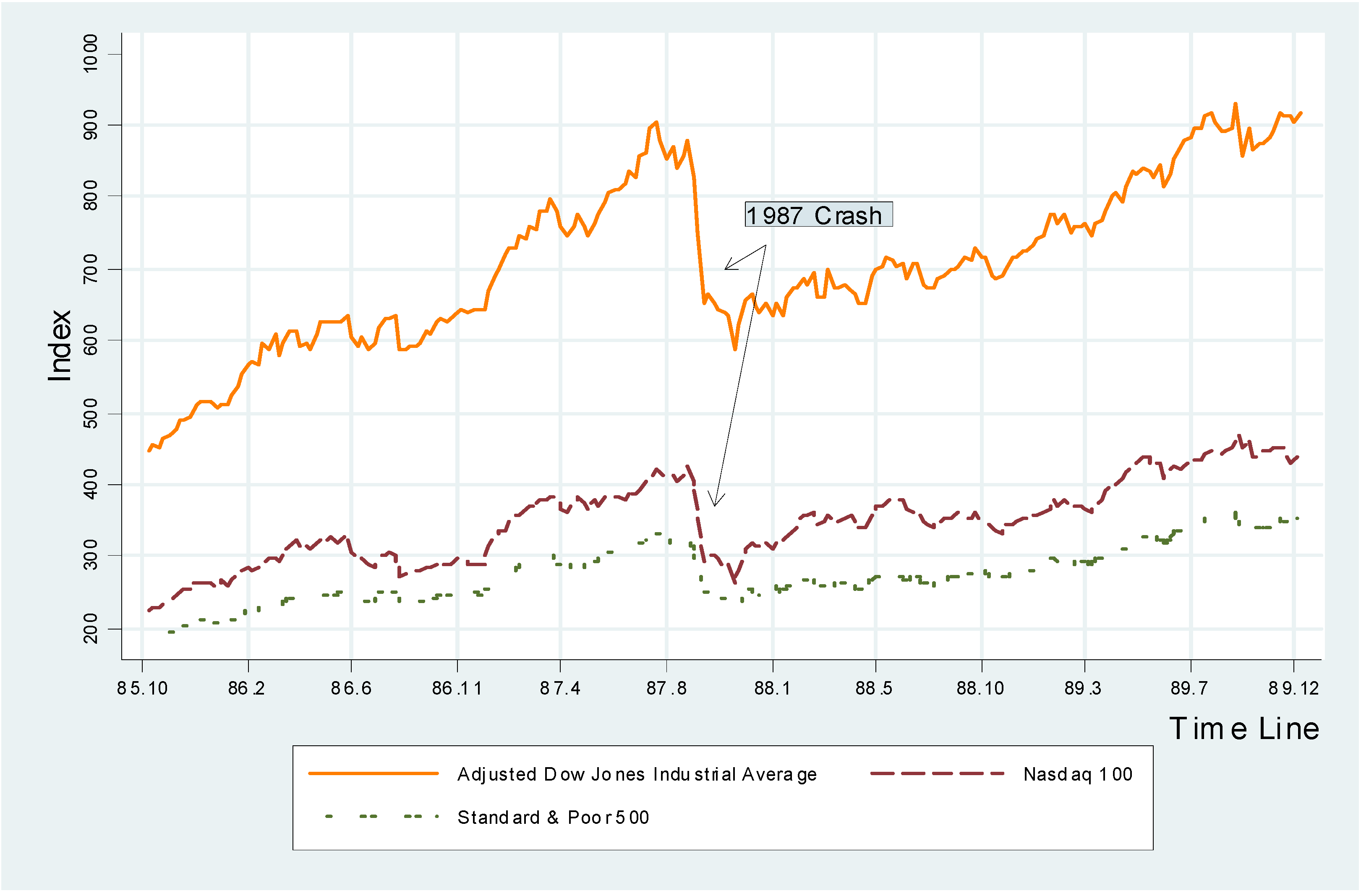
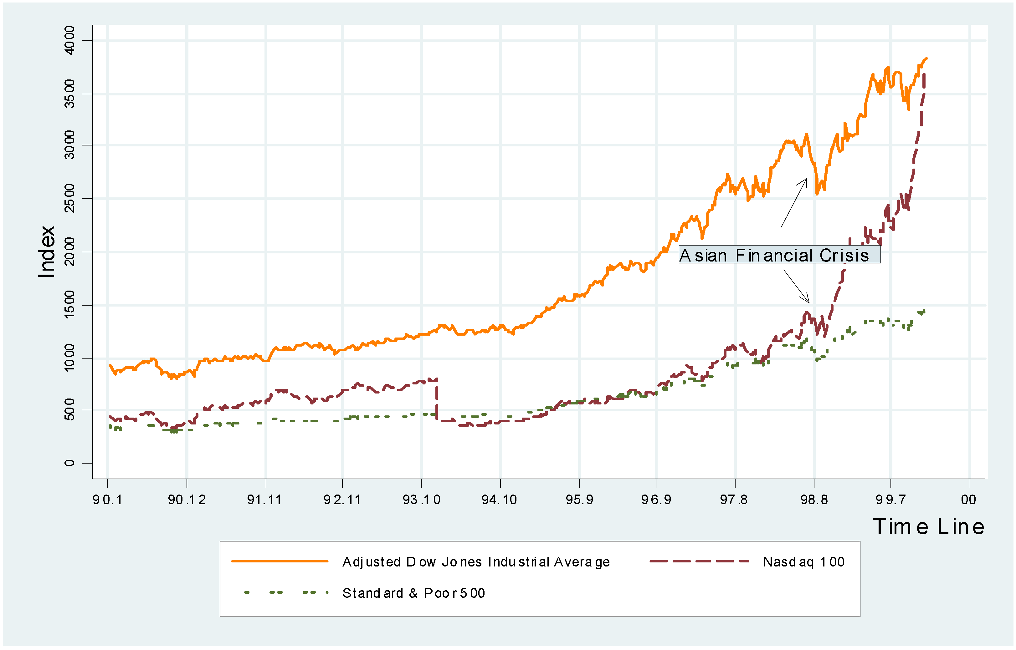
Figure 1,
Figure 2 and
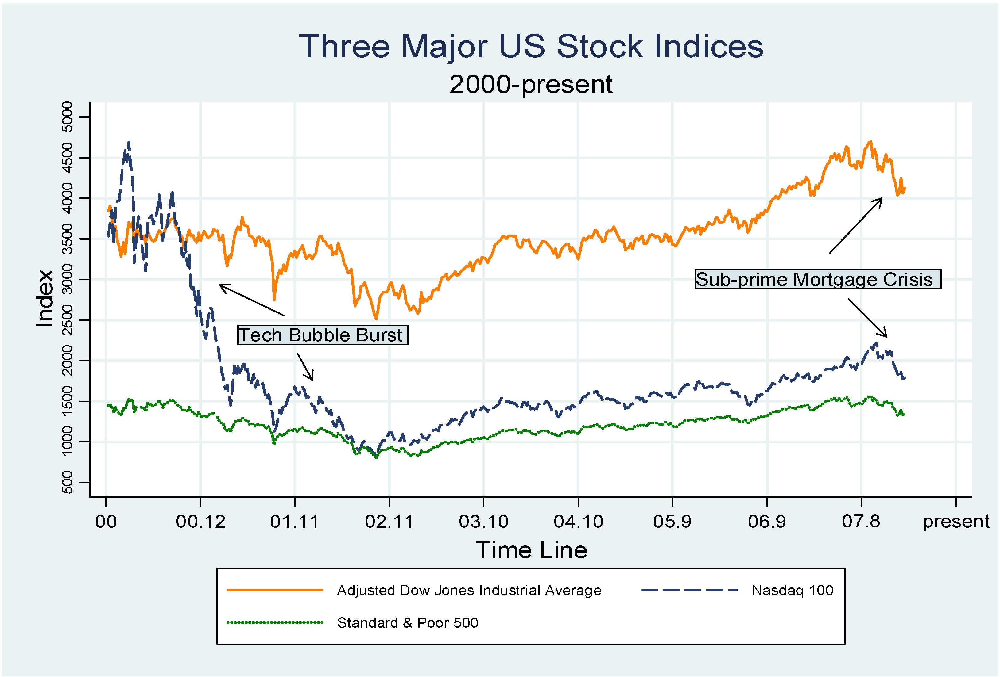
Figure 3 demonstrate the movements of the Dow Jones, Nasdaq 100 and Standard and Poor 500 in three different subsamples from 1985 to 2007.
2 Table 1 summarizes the key features of the three indices.
We modify the Bry and Boschan (1971) algorithm (BB) and use the magnitude of the drop of stock prices in the initial phase to identify stock market crashes.
3 The BB algorithm defines a peak at time t if
and there is a trough at t if
where P
t denotes the value of the stock index at time t. After identifying the peaks and troughs, two criteria are used to determine the starting and ending dates of stock market crashes.
- Criterion 1
All the three indices must fall by more than 30% during the crashes.
- Criterion 2
a. At the beginning of a crash, at least two of the indices reach a two-year high, and at least two of them fall by more than 15% in the following two months.
b. At the end of a crash, at least two of the indices reach a two-year low, and at least two of them rise by more than 15% in the following two months.
Criterion 1 concerns the magnitude of the crash, while Criterion 2 imposes condition on the acuteness of index fluctuation on the starting and ending dates of the crash. Under Criterion 1, two crashes are identified in our sample, namely, the 1987 stock market crash and the tech-bubble burst in 2000-2002. The Asian Financial Crisis in 1997-1998 has a relatively minor impact on the U.S. stock market (all the indices drop by less than 20%). Thus, it is excluded from our analysis. After identifying the two stock market crashes, Criterion 2 is applied to determine the starting and ending dates of the crash periods. The results are reported in
Table 2.
Note from
Table 2 that the duration of the 1987 stock market crash is only three and a half months, while the tech-bubble burst lasts for two and a half years. The starting and ending dates of the two crashes are also identified. As expected, the Nasdaq is more volatile than the other two indices during the tech-bubble burst.
3. ANALYST FORECAST DISPERSION (AFD)
Following the conventional definition of AFD in the literature, we define the analyst forecast dispersion as the standard deviation of earnings forecasts scaled by the absolute value of the mean earnings forecast. To ensure that the AFD is properly defined, we drop the companies covered by less than two analysts. We also follow Sadka and Scherbina (2007) to exclude observations where the mean earnings forecast is zero (which account for 0.07% of the total observations). Finally, following the conventional treatment, stocks with share price lower than five dollars are also removed from our sample. The total percentage of the observations deleted from the original Summary History File is about 28%.
The AFD is a leading indicator that can be used to provide warning signals for market risk. In a risky market, pessimistic analysts are punished less if they remain silent (Jackson, 2005). Thus, we expect the AFD to be considerably lower in the pre-crash period and higher after the crash.
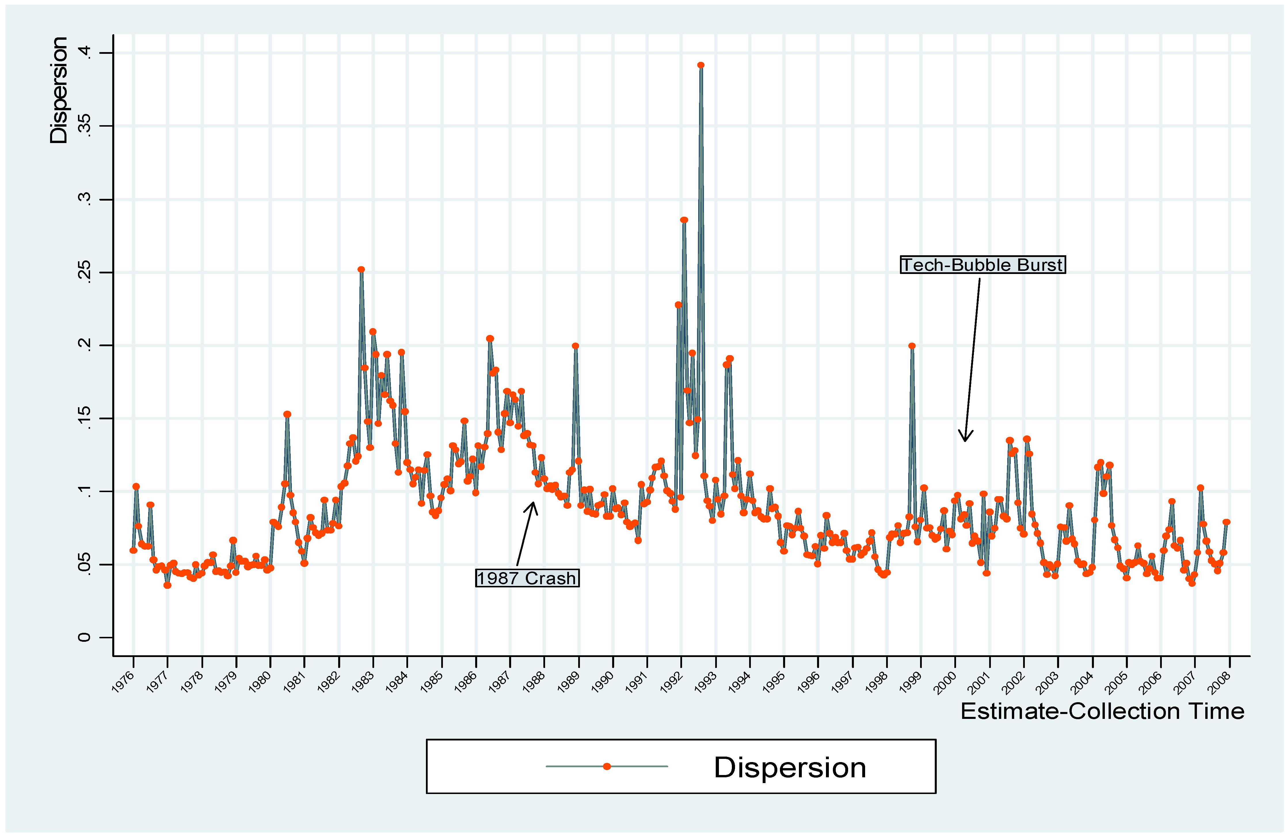
Figure 4 plots the monthly average AFD from January 1976 to December 2007 using the whole sample obtained from the I/B/E/S Summary History Monthly File.
The first observation from
Figure 4 is that the monthly average AFDs at yearends are generally lower than they are in the middle months of the year. The average dispersion is 0.084 for November, December, January and February, while it is 0.094 for May, June and July and August. Furthermore, the AFD exhibits a cyclical pattern. 13 out of 32 (41%) peak in May to August, and 25 out of 32 (78%) AFD annual troughs occur in the months of November to February. Since the duration between the estimate issuance date and forecast end date is shorter at the yearend, it is easier for analysts to reach a consensus based upon information from the final report than that from the interim report, We do not, however, observe abnormal movements of AFD before the two crashes from
Figure 4. The most volatile movements occur at 1982-1984, the end of 1989, 1992-1994, and 1999. We examine the sub-samples covering the two crashes to evaluate the performance of analysts. The monthly average AFDs are depicted in
Figure 5 and
Figure 6.
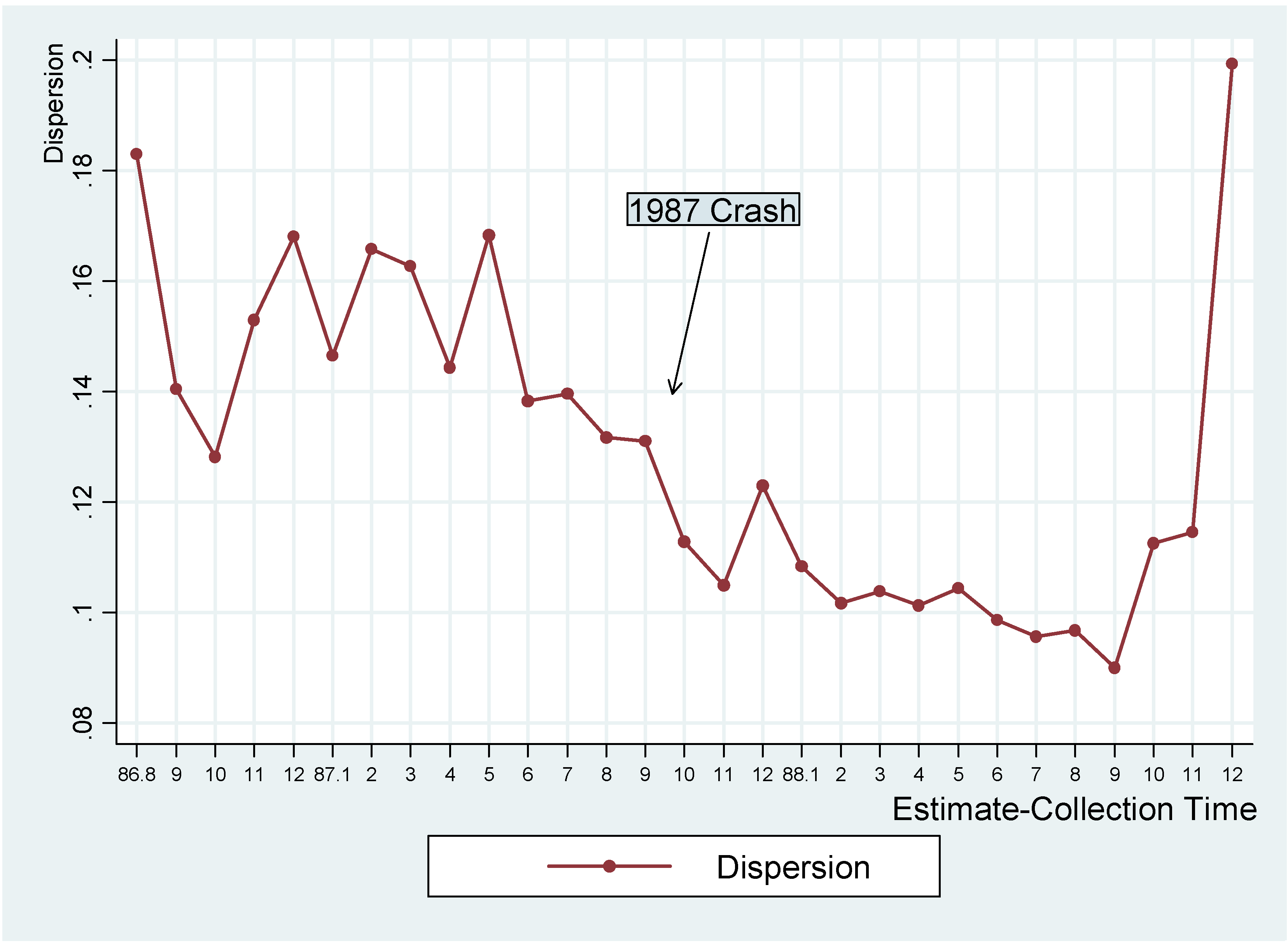
From
Figure 5, we observe a falling AFD before the 1987 crash. In the beginning month of the crash, the AFD is quite stable, but it falls thereafter. In December, the AFD rebounds by 20%, reflecting that analysts have different opinions regarding the ending date of the crash. For the tech-bubble burst,
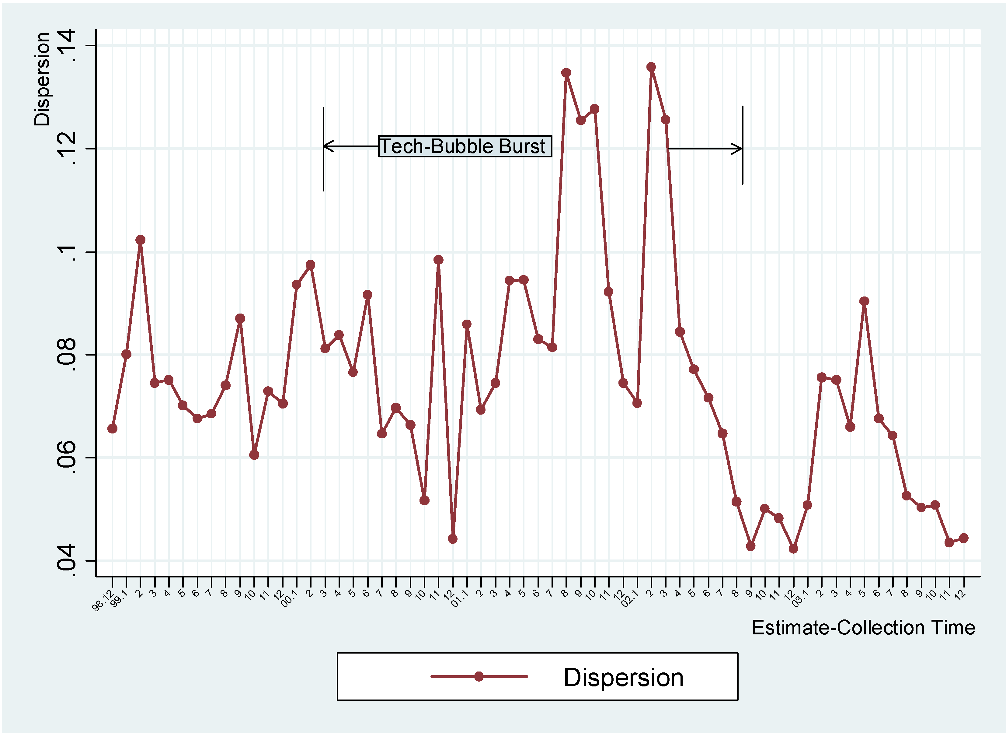
Figure 3 shows that all the indices experience drastic drops and rebounds. This is especially the case for the Nasdaq. The AFD exhibits a downward trend in the first few months of the tech-bubble burst, after which it rebounds rapidly until the end of the burst.
4. FAMA-FRENCH THREE-FACTOR MODEL
To find the relationship between AFD and excess returns in the tech-bubble burst, we incorporate AFD into the Fama-French model.
4 The model of Fama and French (1993) is able to capture the ordering of stock returns across portfolios sorted by variables such as size, B/M, or earning-to-price ratio. Here, we estimate the Fama-French three-factor model for subsamples with different AFDs. First, we sort the stocks in the 2000-2002 sub-sample into five dispersion quintiles, and obtain their average returns. The corresponding excess returns on the left-hand side of the model are derived by subtracting the risk-free rate from the returns obtained. We use the monthly average rate of the one-month U.S. Treasury bill as the risk-free rate.
The three factors are constructed in the same way as Fama and French (1993). The first factor, R
m-R
f, is the excess return on the market portfolio. The second factor, SMB, is the difference between the return on a portfolio of small stocks and that of large stocks. The third factor, HML, is the difference between the return on a portfolio of high book-to-market stocks and that of low book-to-market stocks. The results are reported in
Table 3. The reported t-statistics are Newey-adjusted for heteroskedasticity and serial correlations.
5The results in
Table 3 indicate that the three-factor model leaves a large unexplained return for the portfolio of stocks in the lowest dispersion quintile. Thus, the three-factor model has a lower explanatory power in a rising market where analysts have consensus. Moreover, it is worth noting that, for high dispersion quintiles, the coefficients of HML turn significantly negative.
To examine whether dispersion of analysts’ forecasts can serve as a risk proxy to explain the excess return, we include the average dispersion of the monthly portfolios into the model. If a positive relationship is found, then the AFD can be used as a risk proxy to explain the excess return during stock market crashes. The results are reported in
Table 4. Note that the coefficient of HML becomes insignificant. The R-square of the new model is close to 0.9.
After controlling for market risk, size and book-to-market ratio, the insignificant coefficient of AFD suggests that it is not a good proxy for risk. To allow for nonlinearity, we also include the square of dispersion in the model. The estimation results are reported in the lower panel of
Table 4. The coefficient estimate of squared dispersion is significantly positive, suggesting that excess returns are high when dispersion is too low or too high. Thus, during the crash period, excess returns exist when analysts share that same view, or when they are highly disagree with one another about the prospect of a stock.
5. CONCLUSION
This paper provides a first attempt to study the relationship between the dispersion of analysts’ forecasts and excess stock returns surrounding stock market crashes. We find evidence from the U.S. market that analysts have a bad forecast performance three months before the crashes. We include the AFD and its square in the Fama-French model regression to explain the variation in stock returns during market crashes. It is found that the excess return of a stock has a U-shape relationship with the forecast dispersion of analysts. Thus, in a risky market environment, excess returns can be found in stocks with extreme AFD values.
Table 1.
Summary and Comparison of Three Major U.S. Stock Indices
Table 1.
Summary and Comparison of Three Major U.S. Stock Indices
| | Available since | Covered companies | Characters of companies | Covered Countries | Methodology |
|---|
| DJIA | 1896 | 30 | Largest and most widely held public companies. | U.S. | Price-weighted, scaled if there were stock splits. |
| Nas100 | January 1985 | 100 | Largest domestic and international non-financial companies. | All | Modified value-weighted. |
| SP500 | 1957 | 500 | Large publicly held companies. | Mostly U.S. | Market value-weighted. |
Table 2.
Identification of stock market crashes from 1985 to 2007
Table 2.
Identification of stock market crashes from 1985 to 2007
| | DJ | Nasdaq | SP500 |
|---|
| | Starting | Ending | Starting | Ending | Starting | Ending |
|---|
| 1987 crash | 1987.8.17 | 1987.11.30 | 1987.8.17 | 1987.11.30 | 1987.8.17 | 1987.11.30 |
| Index | 2709.5 | 1766.74 | 421.15 | 260.87 | 335.9 | 223.92 |
| Peak/Trough | Yes | Yes | No | Yes | Yes | Yes |
| % Fall(-)/Rise in 2 months | -28.00 | 10.84 | -30.95 | 22.00 | -26.11 | 15.80 |
| Duration | 3.5 month | 3.5months | 3.5 months |
| % Index change in total | -34.79 | -38.06 | -33.33 |
| 00-02 tech-bubble burst | 2000.3.20 | 2002.9.30 | 2000.3.20 | 2002.9.30 | 2000.3.20 | 2002.9.30 |
| Index | 11112.72 | 7528.4 | 4691.61 | 815.4 | 1527.46 | 800.58 |
| Peak/Trough | No | Yes | Yes | Yes | Yes | Yes |
| % Fall(-)/Rise in 2 months | -7.32 | 18.17 | -33.89 | 36.93 | -19.70 | 17.00 |
| Duration | 2.5 years | 2.5 years | 2.5 years |
| % Index change in total | -32.25 | -82.62 | -47.59 |
Table 3.
Results of Fama-French Three-Factor Models (1999.1 - 2004.1)
Table 3.
Results of Fama-French Three-Factor Models (1999.1 - 2004.1)
| | Factor Sensitivities |
|---|
| Portfolio | Alpha(%) | Rm – Rf | SMB | HML | Adj. R2 |
|---|
| D1(low dispersion) | 1 | 0.722 | 0.253 | 0.084 | 0.73 |
| Newey Adj. t | (3.50) ** | (12.48) ** | (3.71) ** | (4.32) ** |
| D2 | 0.6 | 0.823 | 0.395 | 0.046 | 0.8 |
| Newey Adj. t | (2.60) * | (13.12) ** | (7.39) ** | (2.50) * |
| D3 | 0.3 | 1.016 | 0.537 | -0.032 | 0.85 |
| Newey Adj. t | -0.97 | (12.14) ** | (10.55) ** | (-1.09) |
| D4 | -0.1 | 1.182 | 0.652 | -0.144 | 0.87 |
| Newey Adj. t | (-0.39) | (14.20) ** | (9.20) ** | (-2.83) ** |
| D5(high dispersion) | 0.07 | 1.455 | 0.833 | -0.224 | 0.9 |
| Newey Adj. t | -0.16 | (15.92) ** | (8.14) ** | (-2.86) ** | |
| Tests for ARCH effect and Serial Correlations |
| | ARCH effect | Serial correlation |
| | P-value | P-value | P-value | conclusion | DW statistic | conclusion |
| Regression | (lag1) | (lag2) | (lag3) |
| D1 | 0.94 | 0.31 | 0.36 | No ARCH | 1.57 | Uncertain |
| D2 | 0.94 | 0.62 | 0.7 | No ARCH | 1.56 | Uncertain |
| D3 | 0.6 | 0.91 | 1.21 | No ARCH | 1.77 | No SC |
| D4 | 0.49 | 0.54 | 0.14 | No ARCH | 1.92 | No SC |
| D5 | 0.31 | 0.47 | 0.44 | No ARCH | 1.91 | No SC |
Table 4.
Results of Fama-French Three-Factor Models with Dispersion and its Square(1999.1 - 2004.1)
Table 4.
Results of Fama-French Three-Factor Models with Dispersion and its Square(1999.1 - 2004.1)
| | | Factor Sensitivities |
|---|
| Dep. Variable: excess returns | Alpha(%) | Rm - Rf | SMB | HML | Dispersion | Dispersion2 | Adj. R2 |
|---|
| Loadings | -0.32 | 1.04 | 0.53 | -0.05 | 0.04 | | 0.89 |
| Newey Adj. t | (-0.22) | (16.90) ** | (10.80) ** | (-1.51) | (0.49) | | |
| Loadings | 10.80 | 1.04 | 0.54 | -0.06 | -1.45 | 4.77 | 0.90 |
| Newey Adj. t | (2.01) * | (17.43) ** | (10.08) ** | (-2.77) ** | (-2.09) * | (2.20) * | |
Figure 1.
Three Major U.S. Stock Indices (1985 - 1990)
Figure 1.
Three Major U.S. Stock Indices (1985 - 1990)
Adjusted Dow Jones Industrial Average is derived by dividing the original index by 3, so that it is comparable with the other indices along time.
Figure 2.
Three Major U.S. Stock Indices (1990 - 2000)
Figure 2.
Three Major U.S. Stock Indices (1990 - 2000)
Adjusted Dow Jones Industrial Average is derived by dividing the original index by 3, so that it is comparable with the other indices along time.
Figure 3.
Three Major U.S. Stock Indices (2000 - Present)
Figure 3.
Three Major U.S. Stock Indices (2000 - Present)
Adjusted Dow Jones Industrial Average is derived by dividing the original index by 3, so that it is comparable with the other indices along time.
Figure 4.
Monthly Average AFD (1976.1 - 2007.12)
Figure 4.
Monthly Average AFD (1976.1 - 2007.12)
Figure 5.
Monthly Average AFD (1986.8 - 1988.12)
Figure 5.
Monthly Average AFD (1986.8 - 1988.12)
Figure 6.
Monthly Average AFD (1998.12 - 2003.12)
Figure 6.
Monthly Average AFD (1998.12 - 2003.12)


