

Pricing Path-Dependent Options under Stochastic Volatility via Mellin Transform


Department of Mathematical Sciences, School of Engineering, Computer and Mathematical Sciences, Auckland University of Technology, Private Bag 92006, Auckland 1142, New Zealand
*
Author to whom correspondence should be addressed.
J. Risk Financial Manag. 2023, 16(10), 456; https://doi.org/10.3390/jrfm16100456
Submission received: 15 September 2023
/
Revised: 18 October 2023
/
Accepted: 19 October 2023
/
Published: 20 October 2023
(This article belongs to the Special Issue Featured Papers in Mathematics and Finance)
Abstract
:In this paper, we derive closed-form formulas of first-order approximation for down-and-out barrier and floating strike lookback put option prices under a stochastic volatility model using an asymptotic approach. To find the explicit closed-form formulas for the zero-order term and the first-order correction term, we use Mellin transform. We also conduct a sensitivity analysis on these formulas, and compare the option prices calculated by them with those generated by Monte-Carlo simulation.
Keywords:
asymptotic approximation; barrier; down-and-out; floating strike; lookback; Mellin transform; stochastic volatilityMSC:
91G20; 41A60; 44A99; 91G601. Introduction
A standard option gives its owner the right to buy (or sell) some underlying asset in the future for a fixed price. Call options confer the right to buy the asset, while put options confer the right to sell the asset. Path-dependent options represent extensions of this concept. For example, a lookback call option confers the right to buy an asset at its minimum price over some time period. A barrier option resembles a standard option except that the payoff also depends on whether or not the asset price crosses a certain barrier level during the option’s life. Lookback and barrier options are two of the most popular types of path-dependent options
Following the lead set by Black and Scholes (1973) and assuming that the underlying asset price follows a geometric Brownian motion with constant volatility, Merton (1973) derived a closed-form pricing formula for down-and-out call options. Reiner and Rubinstein (1991) extended Merton’s results to other types of barrier options. Goldman et al. (1979) and Conze and Vishwanathan (1991) provided closed-form pricing formulas for lookback options. For a good summary for research on path-dependent options under the Black–Scholes framework, refer to Clewlow et al. (1994). As we know, the assumption that an asset price process follows a geometric Brownian motion with constant volatility does not capture the empirical observations, due to the volatility smile effect. So, it is desirable to overcome this drawback. There are different ways of extending the Black–Scholes model to incorporate the “smile” feature: one way is to consider “local volatility”, and the other is to consider “stochastic volatility”.
One popular local volatility model is the constant elasticity of variance (CEV) model introduced by Cox (1975, 1996), where a closed-form pricing formula for European call options was presented. Davydov and Linetsky (2001) derived solutions for barrier and lookback option prices under the CEV process in closed form and demonstrated that barrier and lookback option prices and hedge ratios under the CEV process can deviate dramatically from the lognormal values. In Boyle and Tian (1999), the pricing of certain path-dependent options was re-examined when the underlying asset follows the CEV diffusion process, by approximating the CEV process using a trinomial method.
Heston (1993) assumes that volatility reverts to a long-term mean at a specified rate. Bates (1996) builds upon the Heston model by introducing a jump component for asset prices, which is represented as a compound Poisson process with normally distributed jumps. In a further refinement of the Heston model, the jumps are characterized by infinite activity jumps generated by a tempered stable process, as demonstrated in Zaevski et al. (2014). Despite these advancements, the pricing challenges associated with path-dependent options in the context of stochastic volatility persist, as no analytical solutions are available for these models.
Chiarella et al. (2012) considered the problem of numerically evaluating barrier option prices when the underlying dynamics are driven by the Heston stochastic volatility model and developed a method of lines approach to evaluate the price as well as the delta and gamma of the option. Park and Kim (2013) investigated a semi-analytic pricing method for lookback options in a general stochastic volatility framework. The resultant formula is well connected to the Black–Scholes price that is the first term of a series expansion, which makes computing the option prices relatively efficient. Furthermore, a convergence condition for the expansion was provided with an error bound. Leung (2013) and Wirtu et al. (2017) derived an analytic pricing formula for floating strike lookback options under the Heston model by means of the homotopy analysis method. The price is given by an infinite series whose value can be determined once an initial term is given well.
In addition, Kato et al. (2013) derived a new semi-closed-form approximation formula for pricing an up-and-out barrier option under a certain type of stochastic volatility model, including an SABR model. In a more recent paper by Funahashi and Higuchi (2018), a unified approximation scheme was proposed for a single-barrier option under local volatility models, stochastic volatility models, and their combinations. The basic idea of their approximation is to mimic a target underlying an asset process using a polynomial of the Wiener process. They then translated the problem of solving the first hit probability of the asset price into the problem of solving that of a Wiener process whose distribution of the passage time is known. Finally, utilizing Girsanov’s theorem and the reflection principle, they showed that single-barrier option prices can be approximated in a closed form.
The main contribution of this paper is to derive new closed-form approximation formulas for pricing down-and-out put barrier options and floating strike lookback put options under a certain type of stochastic volatility model, which is similar to the one in Cao et al. (2023); Kato et al. (2013); Kim et al. (2023). To achieve our goal, we apply the asymptotic approach discussed in Fouque et al. (2011) and Mellin transform. Mellin transform techniques were used by Panini and Srivastav (2004) to derive integral equation representations for the price of European and American basket put options. Similarly, Yoon (2014) applied Mellin transform to derive a closed-form solution of the option price with respect to a European call option and a European put option with the Hull–White stochastic interest rate. Moreover, Kim and Yoon (2018) derived a closed-form formula of a second-order approximation for a European corrected option price under a stochastic elasticity of variance (SEV) model.
The rest of the paper is organized as follows. Section 2 discusses the model framework and the features of down-and-out and floating strike lookback put options. In Section 3, we provide detailed discussions on an asymptotic approach, which is used to derive approximations to the risk-netural values of these types of options. In Section 4, we apply Mellin transform to derive a closed-form formula of the first-order approximation for down-and-out barrier put options. In Section 5, we apply Mellin transform to derive a closed-form formula of the first-order approximation for floating strike lookback put options. Section 6 presents a sensitivity and comparison analysis and demonstrates that the results given by these closed-form formulas match well with those generated by Monte-Carlo simulation. Section 7 gives a brief summary. Details on Mellin transform and the derivation of the closed-form formulas in Section 4 and Section 5 are provided in Appendix A and Appendix B, respectively.
2. Basic Model Set-Up and Path-Dependent Options
2.1. Stochastic Volatility Model
Let denote the price process of a risky asset on some filtered probability space , where is the physical probability measure In this paper, we assume that evolves according to the following system of stochastic differential equations:
where , , , and m are constants and f is a function having positive values and specifying the dependence on the hidden process . The processes and are independent standard Brownian motions. The constant correlation coefficient with captures the leverage effect. Here, is the drift rate. The mean-reversion process given in Equation (1) is characterized by its typical time to return back to the mean level m of its long-run distribution. The parameter determines the speed of mean-reversion, and controls the volatility of . In the sequel, we shall refer to the above system as the stochastic volatility (SV) model. In Section 2 and Section 3, we will not specify the concrete form of f, but assume that f is bounded and smooth enough, e.g., . Furthermore, f has to satisfy a sufficient growth condition in order to avoid bad behavior such as the non-existence of moments of . For numerical results in Section 6, we choose f to take a special form, as used in Fouque et al. (2000, 2011) and Cao et al. (2021).
We apply the well-known Girsanov theorem to change the physical measure to a risk-neutral martingale measure by letting
where represents the premium of volatility risk. Then, the model equations under the measure can be written as
Note that and are independent standard Brownian motions under . As an Ornstein–Uhlenbeck (OU) process, in Equation (1) has an invariant distribution, which is normal with mean m and variance . Thus, we can expect that if mean reversion is very fast, i.e., goes to infinity, the process should be close to a geometric Brownian motion. This means that if mean reversion is extremely fast, then the model of Black and Scholes would become a good approximation. In reality, however, it may not be the case. For fast but not extremely fast mean-reversion, the Black–Scholes model needs to be corrected to account for the random characteristics of the volatility of a risky asset. For this purpose, we introduce another small parameter defined by , as performed by Fouque et al. (2000). For notational convenience, we put . With the help of these notations, the model equations under are re-written as
where , defined by
is the combined market price of risk.
2.2. Path-Dependent Options
Let denote the payoff of a put option on the risky asset at its expiration T. Then, its risk-neutral price at time under our SV model is given by
Note that depends on the type of options. In this paper, we consider two types of path-dependent options: down-and-out put options and floating strike lookback put options. For notational convenience, we put and . The payoff of a down-and-out put option is given by
where K is the strike price, B is the barrier level satisfying , and is the indicator function. For a floating strike lookback put option, its payoff has the form of . Applying Itô’s lemma, we can obtain a partial differential equation (PDE) for as follows:
The boundary conditions for Equation (3) vary depending on the type of options. For example, the boundary conditions for Equation (3) when are
When , the boundary conditions become the following:
Note that in this case, P is a function of t, s, y, and z (here, ).
Remark: Since the Mellin transform of the payoff function of a call option is not defined, this paper primarily concentrates on evaluating put options. However, as outlined in Buchen (2001), the pricing of call options can be directly derived from put options through the put–call parity relationship.
3. Asymptotic Expansions
In this section, we apply an asymptotic expansion approach to establish partial differential equations, which will be used to derive an approximate solution to Equation (3) and thus find an approximated value of a put option.
We begin with re-organizing Equation (3) in terms of the orders of as follows:
where the operators , and are defined by
In order to obtain an efficient approximate solution to P, as that in Fouque et al. (2011), we apply the following asymptotic expansion of P:
where , , … are functions corresponding to varying orders of . Substituting P in Equation (5) into Equation (4) and re-organizing the terms, we obtain
Our aim is to find and .
Firstly, from the -order term in Equation (6), we obtain . If we assume that does not grow as fast as , as was assumed in Choi et al. (2013), we can show that is independent of y. Secondly, from the -order term in Equation (6), we obtain . Since is independent of y, then . It follows that . Again, if we assume that does not grow as fast as , then we can deduce that is also independent of y.
Next, from the -order term in Equation (6), we obtain
Since is independent of y, we have , which implies that
Seeing Equation (7) as a Poisson equation for in y, in order for it to have a solution, it is required to satisfy the centering condition
which is equivalent to
This is an equation for us to determine the term. Here, denotes the expectation with respect to the invariant distribution of the process , i.e.,
Note that a small value corresponds to fast-mean reverting. In this case, approaches a constant and can be regarded as constant variance, and then Equation (9) is the Black–Scholes PDE. Thus, for small , represents the put option price under the Black–Scholes model.
The solution to Equation (10) can be expressed as
where is a function of y which only satisfies the equation , and c is a function of other variables except y.
To derive an equation for , we consider the -term in Equation (6) and obtain
This equation can be regarded as a Poisson equation for in y, and in order for it to have a solution, the following centering condition must be satisfied:
This is an equation for us to determine the first correction term .
We summarize the previous formal analysis as the following theorem.
Theorem 1.
Under the SV model governed by Equation (1), an approximation of the risk-neutral value P of a path-dependent put option is given by
for small ϵ, where and are determined by Equations (9) and (13) with corresponding boundary conditions, respectively, such that is the put option price under the Black–Scholes model with constant effective volatility and is the first-order correction term.
4. Determining and for Down-and-Out Put Options
In this section, we use Mellin transform to derive analytical expressions of the and terms for down-and-out put options
4.1. Term for Down-and-Out Put Options
In order to use Mellin transform to calculate the term for down-and-out put options, noting that is independent of y under our assumption, we first follow the method in Buchen (2001) and use the boundary condition,
to set up the boundary condition of for as follows:
where . Now, we apply Mellin transform to Equation (9) to convert this PDE into the following ODE:
The solution to Equation (17) is given by
where is a function of w, determined by the boundary condition (16).
Next, we take inverse Mellin transform of Equation (18) and obtain
where
and the operation * means the convolution. Applying Table A1 in Appendix A and the boundary condition given in Equation (16), we have
After some careful calculation, for down-and-out put options, we derive a closed-form expression of the term as follows:
where is the CDF of the standard normal distribution and
4.2. Term for Down-and-Out Put Options
For down-and-out put options, the boundary conditions for are
Next, we apply Mellin transform to Equation (13) to obtain
Solving this equation, we obtain
Finally, applying inverse Mellin transform, we obtain an explicit closed-form expression of as follows:
where is given in the previous section and and are given in Equation (14).
We summarize the above analysis and calculation on down-and-out put options in the following theorem.
5. Determining and for Lookback Put Options
In this section, we use Mellin transform to derive analytical expressions of the and terms for floating strike lookback put options
5.1. Term for Lookback Put Options
For lookback floating strike put options, the boundary conditions of are
Similar to the case of down-and-out put options, we extend the second boundary condition to as follows:
Then, by integrating each side of the last equation, we can obtain
for . For convenience, we let and . With these notations, Equation (9) becomes
with boundary conditions
and , for .
Note that except the boundary conditions, Equation (24) is identical to Equation (9). Applying Mellin transform in the same way as that for the case of down-and-out put options, we can derive the solution to Equation (24) as follows:
After calculating integrals, for floating strike lookback put options, we derive a closed-form expression of the term as follows:
where is the CDF of the standard normal distribution. Note that given in Equation (27) is precisely the same as the price of a floating strike put option given in the literature, e.g., Hull (2015, chp. 26, p. 608) or Haug (2006, chp. 4), if we let . Details of the derivation of this formula can be found in Appendix B.
5.2. Term for Lookback Put Options
For floating strike lookback put options, the boundary conditions for are
Just like that for the -term for floating strike lookback put options, we let and . With these notation changes, Equation (13) is converted to the following:
with for .
Note that Equation (28) is essentially the same as Equation (13), except the notational difference. So, we have
where is given previously. Consequently, we have
where and are the same as those defined previously.
We summarize the above analysis and calculation on floating strike lookback put options in the following theorem.
6. Numerical Results and Sensitivity Analysis
In this section, we conduct a numerical study to investigate the sensitivity of the first-order correction term and our approximation results with respect to the initial value of underlying asset. This means that we set throughout this section. We also compare the results given by our closed form formulas with those generated by the Monte-Carlo simulation.
First of all, as conducted by Fouque et al. (2000, 2011) and Cao et al. (2021), we choose f to take the following form:
Secondly, the values of other parameters used in this section are given in Table 1 whenever they are required to be fixed.
Here, we do not choose precise values of and , and particular forms of (in Section 2) and (in Section 3) to calculate the above values of and . Instead, and are calibrated from the term structure of the implied volatility surface as described in the book of Fouque et al. (2000). Specifically, the implied volatility of a European vallina call option with fast mean-reverting stochastic process can be approximated by the following formula:
with
The parameters a and b are estimated as the slope and intercept of the regression fit of the observed implied volatilities as a linear function of logmoneyness-to-maturity-ratio . From the calibrated values a and b on the observed implied volatility surface, the parameters and are obtained as
Thirdly, note that when , . Hence, in this case, the formula for given by Equation (27) is simplified.
Figure 1a shows how the -term for a down-and-out barrier put option changes with respect to a variation in values As we can see, for fixed , when s increases, decreases first, and then increases after it hits its trough. When becomes smaller (equivalently, the mean-reverting speed becomes larger), approaches to a zero. Figure 1b shows how the value of for a down-and-out put option varies with respect to the change in values. As we can see, when the value of changes from 0.01 to 0.0001, the value of does not vary much. In fact, the values of match well with the result of Monte-Carlo simulation in all cases. Furthermore, in all cases, the value of declines as s increases.
Figure 2a shows how the -term for a floating strike lookback put changes with respect to a variation in values. In a similar pattern, for a fixed -value, when s increases, decreases first and then increases after it hits its trough. Similar to the case of down-and-out put options, when becomes smaller (equivalently, the mean-reverting speed becomes larger), approaches to zero. Figure 2b shows how the value of for a floating strike put varies with respect to the change in values. When the value of changes from 0.01 to 0.001, the value of varies. But when the value of changes from 0.001 to 0.0001, the value of does not vary much. The values of match well with the result of Monte-Carlo simulation when or . Furthermore, in all cases, the value of increases as s increases.
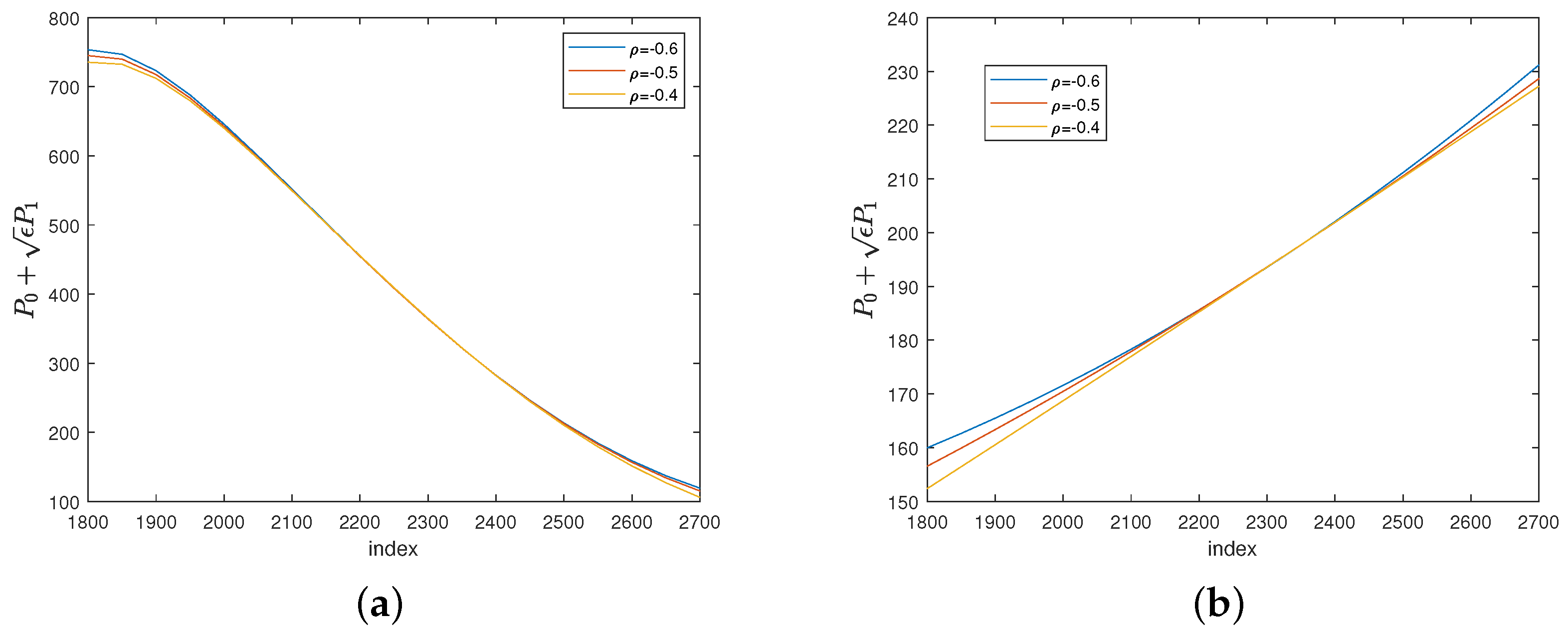
Figure 3a illustrates the variation in the value of for a down-and-out put option in response to changes in values. As shifts from −0.6 to −0.4, there is a slight decrease in the value of . Additionally, in all scenarios, the value of shows an upward trend as s increases.
Figure 3b depicts the change in the value of for a floating strike put concerning variations in values. Similar to the previous case, a shift in from −0.6 to −0.4 results in a minor decline in the value of . Moreover, across all instances, an increase in s is associated with a rise in the value of .
7. Concluding Remarks
This article establishes explicit closed-form solutions for first order approximations of down-and-out barrier and floating strike lookback put option prices under a stochastic volatility model by means of Mellin transform. The zero-order terms in the solutions for the prices of both types of put options coincide with those in Hull (2015) or Haug (2006) under the classical Back–Scholes model. Our numerical analysis shows that the results given by those explicit closed-form solutions match well with those generated by the Monte-Carlo simulation. This confirms the accuracy of the approximation. Furthermore, we also discussed the sensitivity of the first-order error terms and the approximation with respect to the underlying asset price and the mean-reverting speed of the OU-process which governs the volatility.
This model formula can be employed by financial professionals for the swift and precise pricing of barrier and lookback options. This is demonstrated by the efficiency of our formula in comparison to the conventional Monte-Carlo method. Our pricing formula offers an effective means of assessing barrier and lookback options. Looking ahead, we may extend our methodology to evaluate other path-dependent options in future works, including, but not limited to, Asian options, Russian options, and more.
Author Contributions
Conceptualization, J.C.; methodology, J.C. and W.Z.; software, X.L.; validation, J.C. and W.Z.; formal analysis, X.L.; investigation, X.L.; resources, X.L.; data curation, X.L.; writing—original draft preparation, X.L.; writing—review and editing, J.C. and W.Z.; visualization, X.L.; supervision, J.C. and W.Z.; project administration, W.Z.; funding acquisition, J.C. All authors have read and agreed to the published version of the manuscript.
Funding
This research received no external funding.
Data Availability Statement
No new data were created or analyzed in this study. Data sharing is not applicable to this article.
Acknowledgments
The authors would like to thank Jeong-Hoon Kim for valuable discussions and suggestions on Mellin transform method. The authors also thank the anonymous reviewers for their careful reading of our manuscript and their many insightful comments and suggestions.
Conflicts of Interest
The authors declare no conflict of interest.
Appendix A. Mellin Transform
The Mellin transform is an integral transform that may be regarded as the multiplicative version of the two-sided Laplace transform. It is often used in the theory of asymptotic expansions. For a locally Lebesgue integrable function , the Mellin transform denoted by or is given by
and if and c such that exists, the inverse of the Mellin transform is expressed by
In this paper, we use the following properties of Mellin transform.

Table A1.
List of properties of Mellin transform used in this paper.
| Function | Mellin Tansform |
|---|---|
| h | |
Here, , , and are not related to w or s, and , , and are the first-order, second-order, and third-order derivatives of h, respectively.
Appendix B. Derivation of Formulas (20) and (27)
Appendix B.1. Derivation of Formula (20)
From Equation (19), we know that
By letting , we convert the first integral to
we further apply the following changes in variables:
to obtain
Now, if we plug into , , and into the above formula, we derive
Similarly, we can evaluate the second integral
to obtain
Putting these two integrals together yields Formula (20).
Appendix B.2. Derivation of Formulas (27)
From Equation (26), we have
We let . For the first integral, we have
Next, we let
Then, we have
For the second integral, we have
where we use the fact that . Furthermore, we introduce a new variable
Then, we have
Putting these two integrals together and using the fact that , we can obtain our Formula (27).
References
- Bates, David S. 1996. Jumps and stochastic volatility: Exchange rate processes implicit in Deutsche market options. The Review of Financial Studies 9: 69–107. [Google Scholar] [CrossRef]
- Black, Fischer, and Myron Scholes. 1973. The pricing of options and corporate liabilities. Journal of Political Economy 3: 637–54. [Google Scholar] [CrossRef]
- Boyle, Phelim P., and Yisong S. Tian. 1999. Pricing lookback and barrier options under the CEV process. Journal of Financial and Quantitative Analysis 34: 241–64. [Google Scholar] [CrossRef]
- Buchen, Peter. 2001. Image options and the road to barriers. Risk Magazine 14: 127–30. [Google Scholar]
- Cao, Jiling, Jeong-Hoon Kim, and Wenjun Zhang. 2021. Pricing variance swaps under hybrid CEV and stochastic volatility. Journal of Computational and Applied Mathematics 386: 113220. [Google Scholar] [CrossRef]
- Cao, Jiling, Jeong-Hoon Kim, and Wenjun Zhang. 2023. Valuation of barrier and lookback options under hybrid CEV and stochastic volatility. Mathematics and Computers in Simulation 208: 660–76. [Google Scholar] [CrossRef]
- Chiarella, Carl, Boda Kang, and Gunter H. Meyer. 2012. The evaluation of barrier option prices under stochastic volatility. Computers & Mathematics with Applications 64: 2034–48. [Google Scholar]
- Choi, Sun-Yong, Jean-Pierre Fouque, and Jeong-Hoon Kim. 2013. Option pricing under hybrid stochastic and local volatility. Quantitative Finance 13: 1157–65. [Google Scholar] [CrossRef]
- Clewlow, Les, Javier Llanos, and Chris Strickland. 1994. Pricing Exotic Options in a Black-Scholes World. Coventry: Financial Operations Research Centre, University of Warwick, vol. 54, 32p. [Google Scholar]
- Conze, Antoine, and R. Vishwanathan. 1991. Path-dependent options: The case of lookback options. The Journal of Finance 46: 1893–907. [Google Scholar] [CrossRef]
- Cox, John. 1975. Notes on Option Pricing I: Constant Elasticity of Variance Diffusions. Working Paper. Stanford: Stanford University. [Google Scholar]
- Cox, John. 1996. The constant elasticity of variance option pricing model. Journal of Portfolio Management 5: 15–17. [Google Scholar] [CrossRef]
- Davydov, Dmitry, and Vadim Linetsky. 2001. Pricing and hedging path-dependent options under the CEV process. Management Science 47: 881–1027. [Google Scholar] [CrossRef]
- Fouque, Jean-Pierre, George Papanicolaou, and Ronnie Sircar. 2000. Derivatives in Financial Markets with Stochastic Volatility. Cambridge: Cambridge University Press. [Google Scholar]
- Fouque, Jean-Pierre, George Papanicolaou, Ronnie Sircar, and Knut Sølna. 2011. Multiscale Stochastic Volatility for Equity, Interest Rate, and Credit Derivatives. Cambridge: Cambridge University Press. [Google Scholar]
- Funahashi, Hideharu, and Tomohide Higuchi. 2018. An analytical approximation for single barrier options under stochastic volatility models. Annals of Operations Research 266: 129–57. [Google Scholar] [CrossRef]
- Goldman, M. Barry, Howard B. Sosin, and Marry Ann Gatto. 1979. Path dependent options: “Buy at the low, sell at the high”. The Journal of Finance 34: 1111–27. [Google Scholar]
- Haug, Espen. 2006. The Complete Guide to Option Pricing Formulas, 2nd ed. New York: McGraw-Hill. [Google Scholar]
- Heston, Steven. 1993. A closed-form solution for options with stochastic volatility with applications to bond and currency options. The Review of Financial Studies 6: 327–43. [Google Scholar] [CrossRef]
- Hull, John C. 2015. Options, Futures and Other Derivatives, 9th ed. London: Pearson. [Google Scholar]
- Kato, Takashi, Akihiko Takahashi, and Toshihiro Yamada. 2013. An asymptotic expansion formula for up-and-out barrier option price under stochastic volatility model. Japan Society for Industrial and Applied Mathematics Letters 5: 17–20. [Google Scholar] [CrossRef]
- Kim, Hyun-Gyoon, Jiling Cao, Jeong-Hoon Kim, and Wenjun Zhang. 2023. A Mellin transform approach to pricing barrier options under stochastic elasticity of variance. Applied Stochastic Models in Business and Industry 39: 160–76. [Google Scholar] [CrossRef]
- Kim, So-Yeun, and Ji-Hun Yoon. 2018. An approximated European option price under stochastic elasticity of variance using Mellin transforms. East Asian Mathematical Journal 34: 239–48. [Google Scholar]
- Leung, Kwai Sun. 2013. An analytic pricing formula for lookback options under stochastic volatility. Applied Mathematics Letters 26: 145–49. [Google Scholar] [CrossRef]
- Merton, Robert C. 1973. The theory of rational option pricing. Bell Journal of Economics and Management Science 1: 141–83. [Google Scholar] [CrossRef]
- Panini, Radha, and Ram P. Srivastav. 2004. Option pricing with Mellin transforms. Mathematical and Computer Modelling 40: 43–56. [Google Scholar] [CrossRef]
- Park, Sang-Hyeon, and Jeong-Hoon Kim. 2013. A semi-analytic pricing formula for lookback options under a general stochastic volatility model. Statistics & Probability Letters 83: 2537–43. [Google Scholar]
- Reiner, Eric, and M. Rubinstein. 1991. Breaking down the barriers. Risk 4: 28–35. [Google Scholar]
- Wirtu, Teferi Dereje, Philip Ngare, and Ananda Kube. 2017. Pricing floating strike lookback put option under Heston stochastic volatility. Global Journal of Mathematical Sciences: Theory and Practical 9: 427–39. [Google Scholar]
- Yoon, Ji-Hun. 2014. Mellin transform method for European option pricing with Hull-White stochastic interest rate. Journal of Applied Mathematics 2014: 759562. [Google Scholar] [CrossRef]
- Zaevski, Tsvetelin S., Young Shin Kim, and Frank J. Fabozzi. 2014. Option pricing under stochastic volatility and tempered stable Lévy jumps. International Review of Financial Analysis 31: 101–8. [Google Scholar] [CrossRef]
Figure 1.
Plots of and with different values of against the initial value of the underlying asset, for the down-and-out put option.
Figure 1.
Plots of and with different values of against the initial value of the underlying asset, for the down-and-out put option.

Figure 2.
Plots of and with different values of , against the initial value of the underlying asset, for floating strike put options.
Figure 2.
Plots of and with different values of , against the initial value of the underlying asset, for floating strike put options.
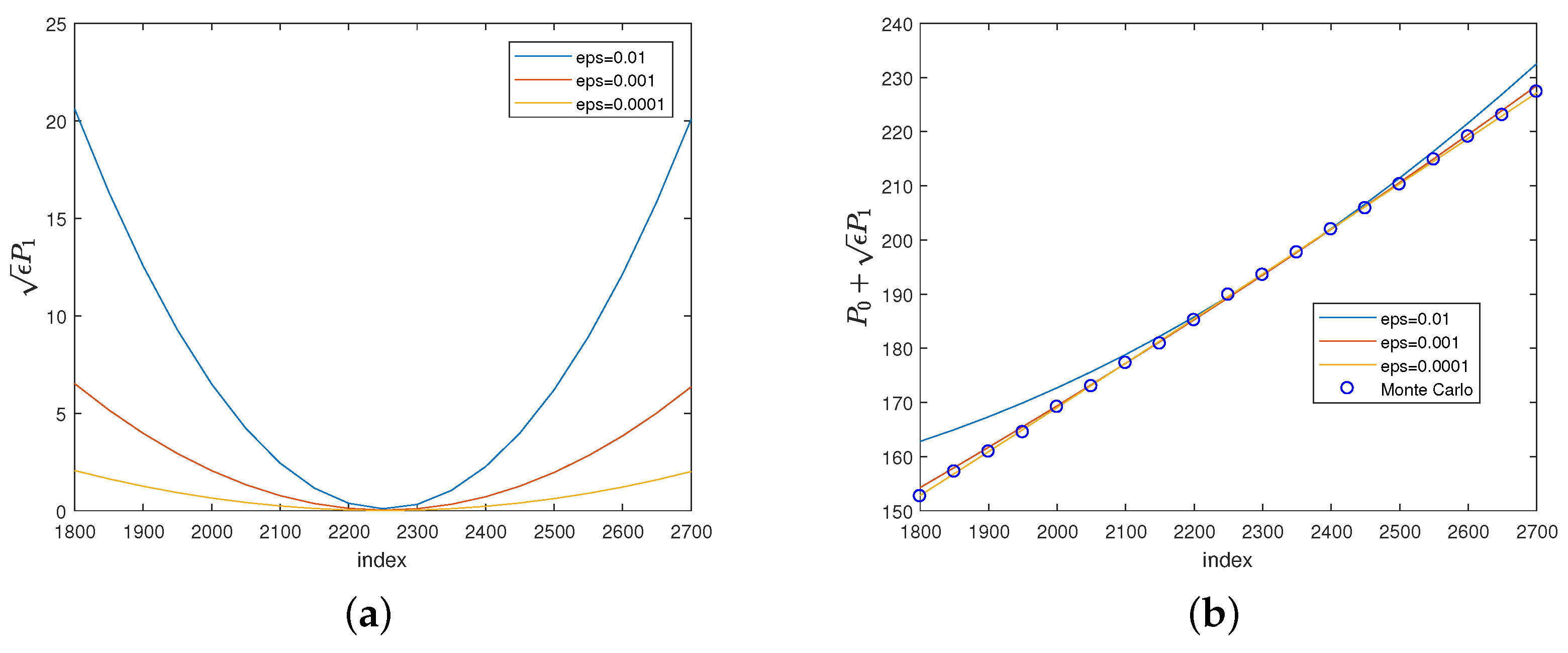
Figure 3.
Plots with different values of , against the initial value of the underlying asset, for down-and-out put option and floating strike put option.
Figure 3.
Plots with different values of , against the initial value of the underlying asset, for down-and-out put option and floating strike put option.
Disclaimer/Publisher’s Note: The statements, opinions and data contained in all publications are solely those of the individual author(s) and contributor(s) and not of MDPI and/or the editor(s). MDPI and/or the editor(s) disclaim responsibility for any injury to people or property resulting from any ideas, methods, instructions or products referred to in the content. |
© 2023 by the authors. Licensee MDPI, Basel, Switzerland. This article is an open access article distributed under the terms and conditions of the Creative Commons Attribution (CC BY) license (https://creativecommons.org/licenses/by/4.0/).
Share and Cite
MDPI and ACS Style
Cao, J.; Li, X.; Zhang, W. Pricing Path-Dependent Options under Stochastic Volatility via Mellin Transform. J. Risk Financial Manag. 2023, 16, 456. https://doi.org/10.3390/jrfm16100456
AMA Style
Cao J, Li X, Zhang W. Pricing Path-Dependent Options under Stochastic Volatility via Mellin Transform. Journal of Risk and Financial Management. 2023; 16(10):456. https://doi.org/10.3390/jrfm16100456
Chicago/Turabian StyleCao, Jiling, Xi Li, and Wenjun Zhang. 2023. "Pricing Path-Dependent Options under Stochastic Volatility via Mellin Transform" Journal of Risk and Financial Management 16, no. 10: 456. https://doi.org/10.3390/jrfm16100456