
The COVID-19 Housing Boom: Is a 2007–2009-Type Crisis on the Horizon?


School of Management, New York Institute of Technology, 1855 Broadway, New York, NY 10023, USA
*
Author to whom correspondence should be addressed.
J. Risk Financial Manag. 2022, 15(8), 371; https://doi.org/10.3390/jrfm15080371
Submission received: 27 June 2022
/
Revised: 12 August 2022
/
Accepted: 15 August 2022
/
Published: 22 August 2022
(This article belongs to the Special Issue Infectious Disease Outbreaks, Uncertainties, Firms, and Financial Markets)
Abstract
:While the current housing market remains relatively strong, with housing prices setting records, concerns are growing of a potential housing bubble similar to that of 2007–2009; this paper compares the current housing market environment with that of 2007–2009 and concludes that the many of the factors that caused the 2007–2009 crisis do not exist today. Factors associated with subprime mortgages, poor and non-existent underwriting loan requirements, weak regulatory oversight, exaggerated credit ratings, under-capitalization in the banking sector and excessive speculative activity in the housing market have been addressed by regulation, which is aimed at preventing another financial crisis similar to 2007–2009. Equally important, major fundamental factors affecting real estate valuation are providing support for the housing market and housing prices; these factors are impacting both the demand and supply side of the housing market. The factors include the lack of inventories of homes available for sale, the underproduction of housing, decreased household mobility limiting supply and the increase in housing demand from millennials and institutional investors; these fundamental factors were not evident during the 2007–2009 period. Despite a number of indicators signaling a potential topping out and overvaluation of housing prices, the authors conclude that the fundamental factors will limit the extent that the housing market weakens over the next few years.
1. Introduction
The US housing market has been significantly impacted by COVID-19, with housing prices reaching record levels. The rate of house price appreciation, which began to accelerate prior to COVID-19 soared during the pandemic as mortgage rates declined to all-time lows. COVID-19 and resulting restrictions lifted housing demand as Americans reconsidered their living arrangements as backyards, and home office space became important.
This spike in housing prices during the pandemic has raised issues of affordability and whether the US real estate market is entering a housing bubble similar to the 2007–2009 experience. In that period, housing prices also surged, increasing home equity and household wealth. When housing prices fell, the equity vanished, pushing the economy into a deep recession. The paper focuses on whether the US is once again in a housing bubble by examining the similarities and differences between the current housing market environment and the housing bubble-associated recession of 2007–2009. We conclude that the underlying causes of the current runup in prices differ from that in 2007–2009, and the current high level of pricing can be explained by fundamentals, which are examined.
The paper is organized as follows: Section 2 provides a literature survey on housing bubbles and looks at the determinants of the 2007–2009 housing crisis. Section 3 looks at the changes in the mortgage financing market and the role of regulatory changes. Section 4 focuses on the current market conditions and the long-term trends in supply and demand. Section 5 looks at some indicators that function as warning signals of trouble brewing in the housing market. Finally, Section 6 provides conclusions.
2. Literature Survey
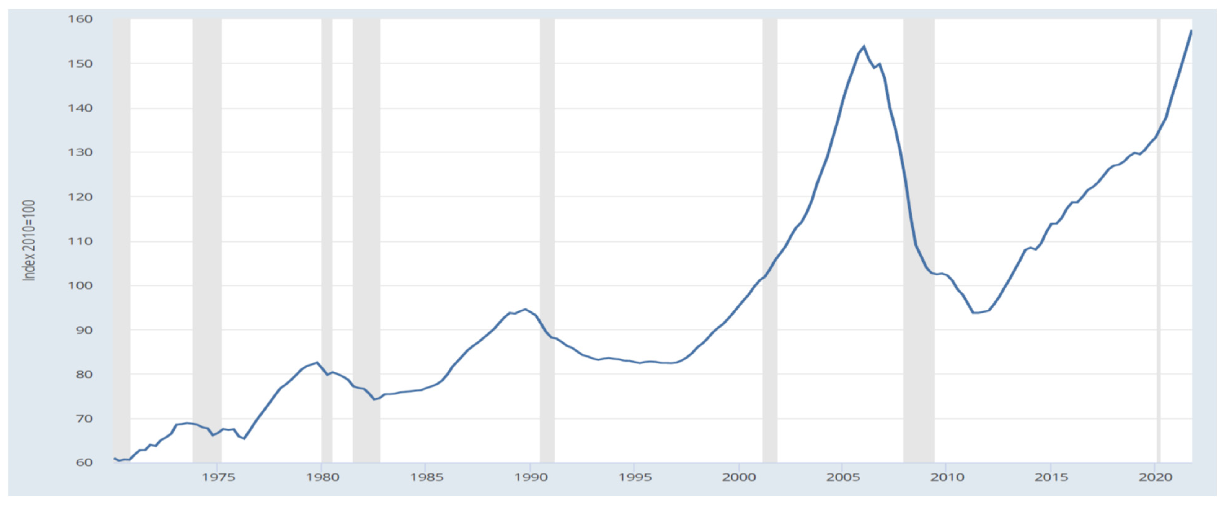
The state of the housing market can be evaluated by analyzing various house price indices measured in either nominal or real terms. To get a picture of the US housing market, Figure 1 looks at the real housing price data from the BIS (Bank of International Settlement) since 1970. Over the 28-year period between 1970 and 1998, real US housing prices showed a modest upward trend with moderate declines occurring during periods of recession. Between 1970 and 1998, real housing prices rose cumulatively by 44.2% or at an average 1.3% annual rate; this housing market dynamic began to change in the late 1990s. Home prices showed strong increases starting in 1998, with prices rising significantly through the 2001 recession and during the sluggish recovery of the early 2000s. During this period, the rise in home prices was attributed to strong market fundamentals, an increase in family income and declines in mortgage interest rates (McCarthy and Peach 2004).
Housing prices continued the rapid upward trend reaching a peak in 2006. In real terms, housing prices rose cumulatively by 72.4%, or by an average 7% annual rate, between 1998 and 2006. The house price runup from 2001 to 2006 is attributed to the declining mortgage rates (Taylor 2009; Himmelberg et al. 2005) and relaxed credit constraints (Mian and Sufi 2009; Glaeser et al. 2010; Favilukis et al. 2010; Demyanyk and Van Hemert 2011). The relaxed credit conditions created a leverage cycle (Geanakoplos 2010). A leverage cycle occurs when leverage gradually rises too high and then suddenly falls too low. Haughwout et al. (2011) provided evidence of the existence of a leverage cycle in the housing market by showing that investors buying multiple homes grew from around 20% in 2000 to nearly 35% in 2006. Similarly, Chinco and Mayer (2016) attributed the price increases to the increase of out-of-town second house buyers that they call distant speculators; these distant speculators entered the market in larger numbers just prior to the house price peak and inflated house prices.
COVID-19 caused additional risk and uncertainty in the market, which affected investors’ assessment of the benefits and the costs associated with investment decisions. A key variable impacting the investment decision is the discount rate, which is used to determine the present value of the future cash flows. One of the primary determinants of the discount rate is the level of interest rates. The problem is that during periods of uncertainty interest rates are volatile; this volatility in interest rates makes estimating the discount rate difficult and may result in errors in calculating the profitability of an investment decision (Drozdowski 2021).
Additionally, banks played a role in the housing market crisis. According to Stiglitz (2009) banks did not understand the extent of the risks that were created by securitization, by incorrectly assessing the risks associated with new financial products of low- or no-documentation loans and underestimating the risks associated with real-estate price declines. Rajan (2006) predicted that these changes in the financial sector created greater financial risk and greater probability, even though small, for a catastrophic meltdown. The catastrophic meltdown occurred with the burst of the housing bubble.
2.1. Subprime Mortgages
At the core of the crisis was the significant rise in the use of subprime mortgages. A subprime mortgage is generally defined as a non-traditional, riskier type of loan due to factors such as a low initial home down payment, low borrower credit score, high debt ratio, high debt to income ratio, previous late debt payments and/or previous bankruptcy proceeding(s); this type of loan is characterized by a higher interest rate assessment in order to compensate the lender for the increased risk of default on the mortgage. Subprime loans originated in 1982 when Congress passed the Alternate Mortgage Transactions Parity Act (AMTPA), which allowed non-federally chartered housing creditors to write adjustable-rate mortgages with the goal of increasing home ownership in the US; these mortgages were non-conforming with the strict government agency standards as were applicable to the Fannie Mae and Ginny Mae regulatory criteria. Instead, they were based on lax underwriting requirements, often requiring a minimal or no down payment and payable on an adjustable-rate basis which was originally set at a level well below market.
The proliferation of subprime mortgages from 2004–2007 was in reaction to the developing influx of money to the private sector beginning in the early 2000s. The investment banks on Wall Street met this demand by the creation of newly minted subprime debt products, such as Mortgage-Backed Securities (MBS) and Collateralized Debt Obligations (CDO), which inexplicitly were assigned as investment grades by the Big Three credit rating agencies. To produce more mortgages in the 2004–2007 period, there was an abrupt decline in mortgage qualification guidelines. First, “stated income, verified assets” (SIVA) loans replaced proof of income with a “statement” of it. Then, “no income, verified assets” (NIVA) loans eliminated proof of employment requirements. Borrowers needed only to show proof of money in their bank accounts. “No Income, No Assets” (NINA) or Ninja loans eliminated the need to prove or even to state any owned assets. All that was required for a mortgage was a credit score (Zandi 2009). Additionally, the use of automated loan approvals which became the norm for underwiring these mortgages, allowed loans to be made without appropriate review and documentation (Ward 2004).
A high percentage of the subprime mortgages were adjustable, with over 90% of the loans made in 2006 having an interest rate feature that increased over time. The interest-only adjustable-rate mortgage (ARM), which became popular during this period, allowed the homeowner to pay only the interest (not principal) of the mortgage during an initial “teaser” period. Nearly 25% of all mortgages made in the first half of 2005 were “interest-only” loans (FDIC 2006). More lenient was the “payment option” loan, in which the homeowner had the option to make a monthly payment that did not even cover the interest for the first two- or three-year initial period of the loan. Nearly one in 10 mortgage borrowers in 2005 and 2006 took out these “option ARM” loans (Knox 2006) and an estimated one-third of ARMs originating between 2004 and 2006 had "teaser" rates substantially below the prevailing market mortgage interest rate. After the initial “teaser period”, monthly payments typically more than doubled and often tripled, while many also resulted in an increased amount of the outstanding principal loan balance (negative amortization). In addition to considering higher-risk borrowers, lenders offered overly luxurious borrowing terms. In 2005, the median down-payment for first-time home buyers was 2%, with 43% of those buyers making no down payment whatsoever (Knox 2006); this action resulted in an overly speculative strategy in the housing market as the upside for potential gains as witnessed by purchasers in 2004–2006 was unlimited, while losses, as witnessed by purchasers in 2006–2007, were minimal or non-existent; this created a unique favorable arbitrage type “win only no-lose” opportunity for home buyers. The above-aforementioned items resulted in a drastic increase in the percentage of lower quality subprime mortgages from a historical 8% or lower range to approximately 20% from 2004 to 2006, with much higher ratios in some parts of the U.S. (Simkovic 2013).
2.2. Predatory Practices
Predatory practices are defined as unfair, deceptive, and/or fraudulent practices of lenders during the loan origination process; these practices were commonplace during 2004–2006 as lenders made loans that they knew borrowers could not afford and would not be able to repay. The chairman on the Mortgage Bankers Association claimed that mortgage brokers while profiting from the home loan boom, did not do enough to examine whether borrowers could repay their mortgage obligations. “Lenders made loans that they knew borrowers could not afford and that could cause massive losses to investors in mortgage securities” (Government Publications 2011). Additionally, due to weak and arguably non-existing regulatory consumer protection laws, lenders were not required to adequately disclose the risks and the makeup of the loan product(s) to the borrowers.
2.3. Credit Agencies
The Big 3 rating agencies which include Moody’s Investor Services, Standard and Poor’s and Fitch, rate securities by assessing the ability of the debtor to repay their future interest and loan obligations. Investors place significant reliance on such ratings in their investment decision process and in the formulation of their risk-return tolerance level, which is the core of modern portfolio theory. The subprime mortgage-backed securities from the 2004–2008 period were generally rated as investment grade by each of the Big 3 rating agencies, implying a low degree of credit risk and as such, tailored-made for conservative investors. From 2000 to 2007, Moody’s rated nearly 45,000 mortgage-related securities, with more than half of those rated as triple-A (Benmelech and Dlugosz 2009).
By the end of 2008, 80% of the CDOs by value rated “triple-A” were downgraded to junk (later termed as “toxic”) (Smith 2008), resulting in bank write-downs and losses on these investments of USD 523 billion (Birger 2008). What followed was a series of bankruptcy proceedings to many investors which included “investment giant” Lehman Brothers and extending to a host of global sovereignties who invested heavily in these vehicles. The defense by the Big 3 was that they should not bear any responsibility or accountability as their proprietary methods of assigning a rating score is based on historical and not on prospective factors. The Big 3 articulated in their defense that prospective factors which may affect the ability for a debtor to pay off future debt are not presently known and thus not predictable. Despite this questionable defense, the Big 3 paid a significant amount to settle their lawsuits (in excess of USD 1.3 billion), and many insiders faced criminal charges from the Securities and Exchange Commission (SEC), which never materialized to any meaningful level.
2.4. Results
The combination of lax underwriting requirements, low or no down payment on home purchases and low initial mortgage payments during the 2 to 3 “teaser period” created a very high-risk scenario in the collateralized mortgage obligation market. Non-payment of the mortgages would force delinquencies followed by the bank repossession process. In the best-case scenario, if home prices increased coupled with lower adjustable reset interest rates, the owner would profit from their actions. U.S. home prices, however, declined steeply after peaking in mid-2006. Additionally, adjustable-rate mortgages began to reset at much higher interest rates leading to delinquencies. The result of a low or no down-home payment, combined with a significantly higher mortgage payment and lower home prices resulted in homeowners abandoning their homes and the start of an epidemic involving bank repossessions; this level of foreclosure activity was not witnessed in the US in any prior period and was the main catalyst of the deep worldwide recession that followed. All the factors that appeared favorable in 2004–2006 proved to be catastrophic in 2007–2009.
2.5. Housing Prices
Historically, the cyclical behavior of housing prices is measured based on fundamentals. Fundamentals measure house prices relative to the present value of rents, construction costs, and economic fundamentals such as income, population and employment. Prices rising more than fundamentals would suggest a boom and prices falling faster than the decline in fundamentals would indicate a bust (Mayer 2011). The economic theory of rational individual behavior excludes the possibility of the existence of bubbles. A bubble exists when investors believe that the selling price will be higher tomorrow, but fundamental factors do not justify the price increases (Stiglitz 1990). Glaeser et al. (2008) found that housing bubbles are correlated with the elasticity of supply of houses. Markets with elastic housing supply have fewer and shorter bubbles with smaller price increases. Housing fundamentals, cost, and housing supply do not capture the whole picture in regard to housing prices. Many researchers point to rational exuberance. Case and Shiller (1989) were the first to report that housing prices do not follow a fully rational pattern and thus are not very forecastable. Irrational beliefs by many that home prices could only go up as well as the widespread perception that houses are a great investment contributed to a housing price boom (Akerlof and Shiller 2009; Shiller 2007).
Another market inefficiency that can affect housing prices is money illusion. People or investors suffering from money illusion tend to inversely value an asset relative to inflation. For example, when inflation declines they tend to underestimate the real cost of future mortgage payments thus causing upward pressure on housing prices (Brunnermeier and Julliard 2008). Nevertheless, money illusion is not a factor that differentiates the current cycle from the 2007–2009 housing bubble.
3. Regulation
Due to the financial crisis of 2007–2009, The Dodd–Frank Wall Street Reform and Consumer Protection Act was enacted on 21 July 2010. The Dodd–Frank Act, which has changed the lexicon of subprime mortgages to “non-qualified,” addressed the many issues described above, and its regulatory goals, which are discussed next, included: 1—preventing predatory lending practices, 2—strengthening mortgage underwriting requirements, 3—limiting speculative investments by the banking sector, 4—placing greater accountability on the part of the Big 3 credit companies, and 5—provide financial stability oversight over major financial institutions.
1—Preventing Predatory Lending Practices: Dodd–Frank established the Consumer Financial Protection Bureau (CFPB). The role of the CFPB is to prevent predatory lending practices by requiring full disclosure to the borrower. The disclosure should be in an easy-to-read format ensuring that the customer fully understands the mortgage terms prior to agreeing to them. The CFPB also requires that anyone who obtains a subprime home loan undergo homebuyer counseling by an approved representative from the Department of Housing and Urban Development (HUD) agency; it also precludes mortgage brokers from recommending products which are not suitable to the consumer, which is often done for the pursuit of earning additional commissions. The CFPB legislation also extends to other loans, such as credit card and debit cards and will investigate consumer complaints against lending institutions. In closing, the CFPB oversees consumer financial markets with the goal of ensuring that the prices, risks and terms of loan deals are clear at the beginning of the process so that consumers can fully understand their options prior to commitment.
2—Underwriting requirements are strengthened significantly: Dodd–Frank standards require lenders to abide by the “ability-to-repay” (ATR) provision, which comprehensively assesses whether the borrower can repay the loan. For adjustable loans, the underwiring requirement is to base the customer’s relevant income to debt ratios on the highest possible adjustable reset rate. Failure by the lender to satisfy the ATR standards are subject to regulatory penalties. Additionally, down payments for subprime mortgages now exceed traditional loan amounts for home purchases; this limits the use of a speculative strategy in the real estate industry. As such, Mortgage loans are more difficult to obtain as they are based on the consumer’s ability to repay the loan.
3—The Volcker Rule has restricted how banks can invest by limiting speculative investments and eliminating proprietary trading. The Volcker rule has the effect of materially limiting the proliferation of subprime securities in the marketplace.
4—The Securities and Exchange Commission’s (SEC’s) Office of Credit Ratings is charged with ensuring oversight over rating agencies. Rating agencies are required to provide meaningful and reliable credit ratings of the entities that they evaluate.
5—The creation of the Financial Stability Oversight Council and the Orderly Liquidation Authority, which monitor the financial stability of major financial firms which are “too big to fail”, as the failure of such companies could have a serious negative impact on the U.S. economy.
To further solidify the prevention of “too big to fail”, the Dodd–Frank Act mandated the Federal Reserve to more closely oversee large banks, financial institutions and insurance companies in the U.S. As a result, federal and financial authorities greatly expanded regulatory reporting requirements to focus on the adequacy of capital reserves and internal strategies for managing capital. Banks must regularly determine their solvency and document it (FRB-Dodd–Frank Stress Test). The “stress test” evaluation became effective in 2011 when the Federal Reserve instituted regulations that required banks to perform a Comprehensive Capital Analysis and Review (CCAR), which includes running various stress-test scenarios (ECB 2021).
Company-run stress tests are conducted on a semiannual basis and fall under tight reporting deadlines and are conducted under hypothetical scenarios designed to determine whether a bank has enough capital to withstand a negative economic shock(s); these scenarios include unfavorable situations, such as a deep recession or a financial market crash. In the United States, banks with USD 250 billion or more in assets are required to undergo internal stress tests conducted by their own risk management teams and the Federal Reserve (The Federal Reserve (n.d.) Dodd–Frank Act Stress Test Publications). If it is shown that a company does not have met adequate capital in reserves to overcome certain scenarios, the Federal Reserve can take various actions to safeguard the bank and minimize the possible negative effects on the US economy; this includes the appointment of a receivership and/or reorganization proceedings.
Stress tests focus on a few key areas, such as credit risk, market risk and liquidity risk to measure the financial status of banks in a crisis. Using computer simulations, hypothetical scenarios are created using various criteria from the Federal Reserve and International Monetary Fund (IMF). The European Central Bank (EBC) also has strict stress testing requirements covering approximately 70% of the banking institutions across the eurozone (ECB 2021). All stress tests include a uniform set of scenarios that banks may experience. The variables incorporating the stress test evaluation include: Gross Domestic Product (3 input’s-real, nominal and growth), nominal disposable income, unemployment rate, interest rates (5 inputs-3 month, 5- and 10-year Treasury rates, the BBB corporate yield and the prime rate), inflation rate (CPI) and 3 levels- the Dow Jones Total Stock Market, Market Index House Price Index and the Commercial Real Estate Price Index Market Volatility Index.
To further supplement Dodd–Frank regulation, in July 2013, the Federal Reserve finalized a rule to implement the Basel III Accord in the US. Basel III is an international standard published by the Basel Committee on Banking Supervision in November 2010. Basel III, which builds on the previously mandated Basel I and II standards, significantly increases the minimum capital requirements (tier 1, tier 2, and total). Basel III also introduced new rules requiring that banks maintain additional reserves known as countercyclical capital buffers (CCB), which is essentially a “stress test “type reserve to absorb the effects of a potentially catastrophic event(s); it also strengthened the liquidity position of financial institutions by the creation of a minimum liquidity reserve, which requires financial institutions to hold a minimum amount of high-quality liquid assets which can be converted into cash easily, quickly and with a minimum risk of loss.
3.1. Minimum Capital Requirements under Basel III
Banks have two main classifications of capital whose functions differ from one another. Tier 1 capital includes the bank’s core capital, equity and the disclosed reserves that appear on its financial statements. If a bank experiences a significant loss, Tier 1, termed as “going concern capital” provides a buffer that will allow it to sustain losses and maintain its continuity of business operations. The minimum tier 1 capital requirement is 6% of risk-weighted assets. (RWA). By contrast, tier 2 refers to a bank’s supplementary layer of capital known as “gone capital”, and is composed of items such as revaluation reserves, hybrid instruments, off balance sheet assets/debt and subordinated term debt; it is considered less secure than tier 1 capital and more difficult to liquidate. The minimum capital requirement of tier 1 and tier 2 assets is 8% of the risk-weighted assets (RWA); it is critical to note that the denominator in each of these ratios is an item known as risk-weighted assets (RWA).
Risk-weighted assets is a measure of the risk inherent in a bank’s assets, which is essentially its holding in the loan portfolios. All else equal, a risker type asset is assigned a higher risk-weighted asset value resulting in a lower capital ratio, whereas a lower risk asset will result in a lower risk-weighted asset value and thus a higher capital ratio. Low-risk assets include investments in Treasury bills and collateralized assets, whereas uncollateralized assets and off-balance sheet debt represent higher type risk assets. The standard of measuring minimum capital ratios on the basis of the riskiness of a bank’s asset holdings significantly precludes a bank from an overly aggressive speculative investment strategy.
Federal Reserve regulations require banks to value securities consistent with the provisions of Accounting Codification Standard (ASC) 820 Fair Value Measurements. The implementation of ASC 820 which became effective post the housing boom (beginning on 1 January 2008 for calendar year entities), further insulates the recurrence of a 2004–2009 type housing boom and resulting recession.
3.2. Major Provisions of ASC 820
1—ASC 820 defines Fair Value as “the price that would be received to sell an asset or paid to transfer a liability in an orderly transaction between market participants at the measurement date” (FASB 2018). Fair value is the price to sell an asset or transfer a liability and, therefore, represents an exit price, not an entry price. An exit price criterion as required by ASC 820 guidance will normally discount an asset value which lacks an active trading market, known as lack of marketability, significantly; this discount typically represents a greater than 25% amount of asset value; this can be observed for example on how the Internal Revenue Service (IRS) values assets by the application of IRS Revenue Ruling 59-60, 19591, CB 237-IRC 2031, which commonly results in a greater than 25% discount for non- marketable assets.
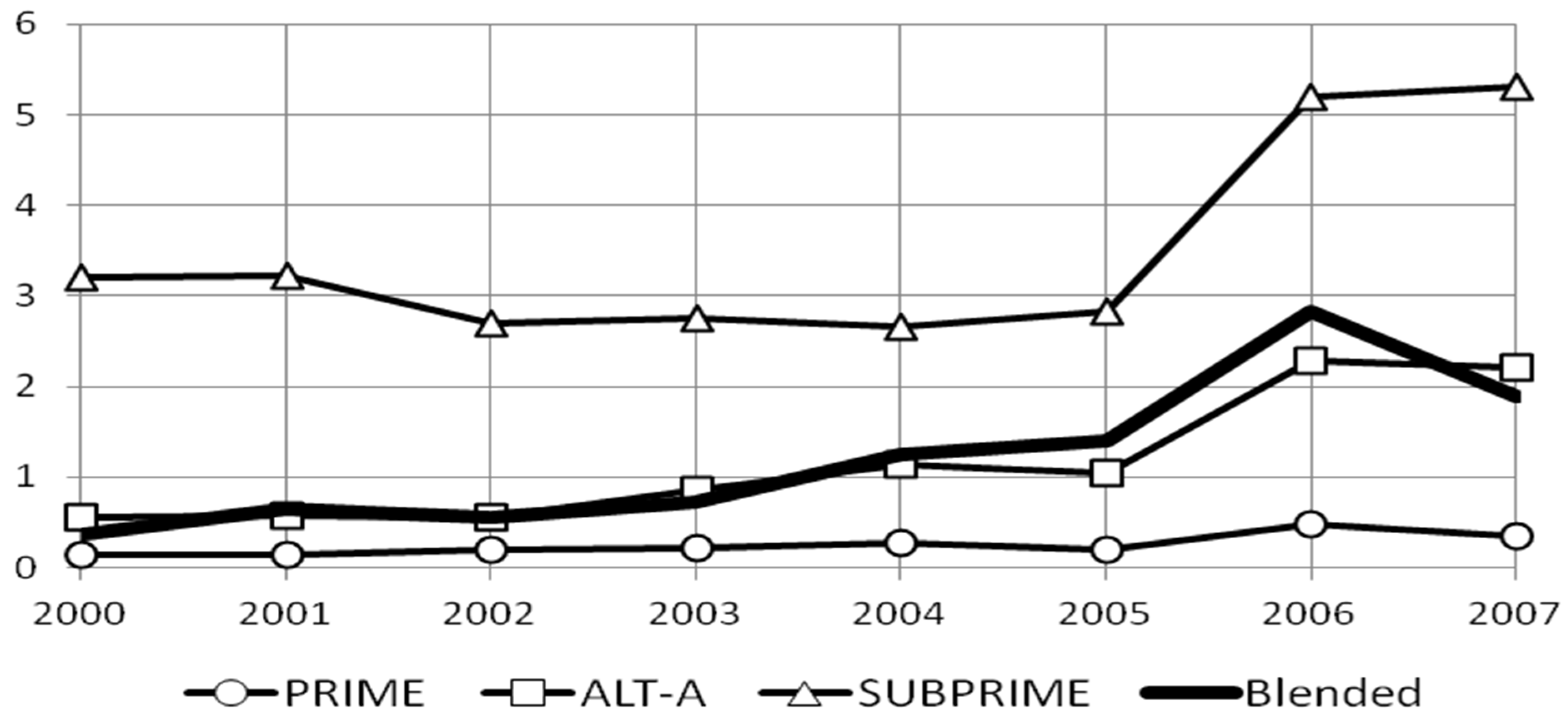
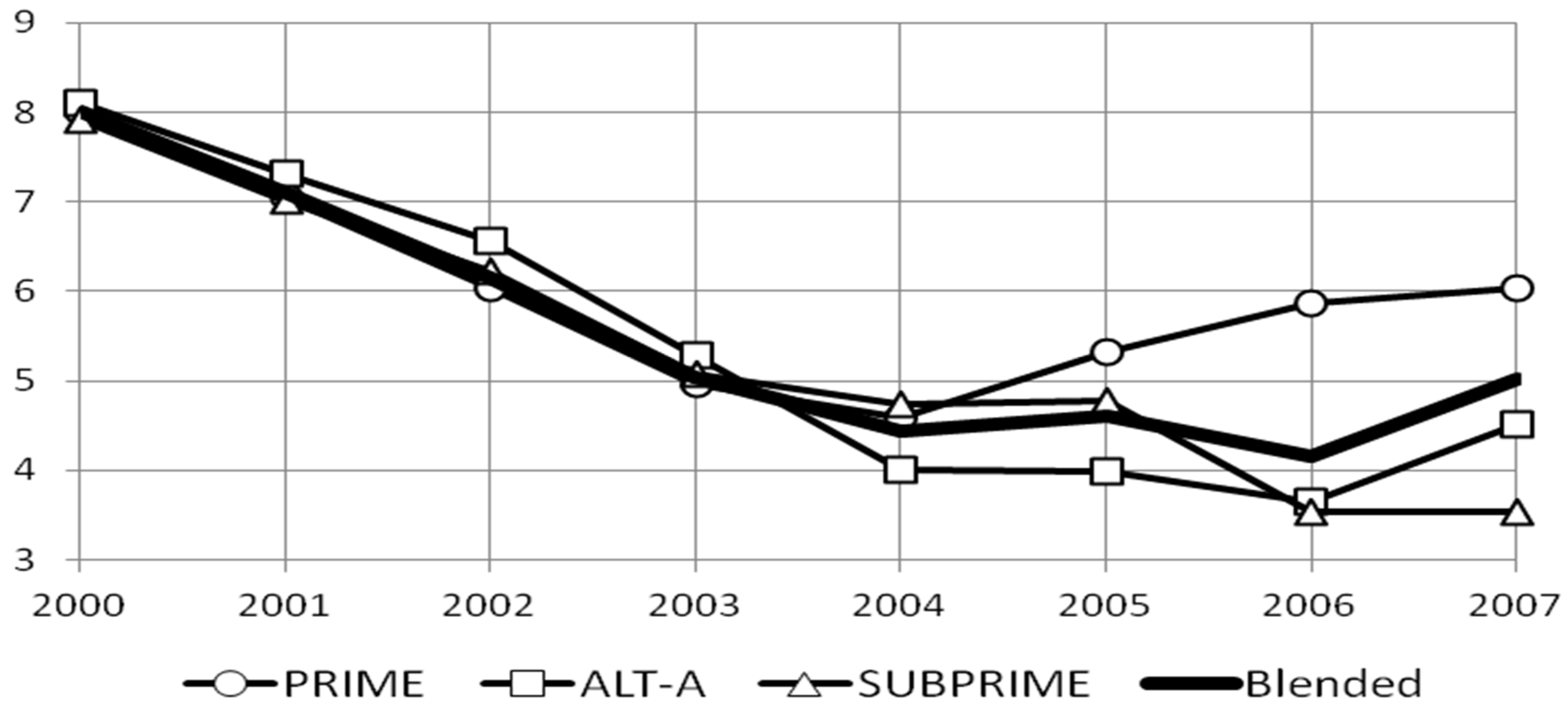
2—Fair value is a market-based measurement, not an entity-specific measurement, and as such is determined on the basis of market participant pricing assumptions. As such, unobservable inputs (e.g., use of a reporting entity’s own data/input) should be minimized and the use of observable inputs should be maximized. The valuation of the 2004–2008 subprime mortgage assets were based on managerial and not market- based assumptions. Figure 2 reflects the annual loss rate on mortgages and Figure 3 provides the loss-adjusted coupon rate of mortgages from 2000 to 2007. Based on findings by Davison et al; moreover as shown in Figure 3, prior to 2004, loss-adjusted rates had been similar among prime (conforming), Alternative A-paper (CMO’s with risks in between prime and subprime), and subprime mortgages suggesting that the risk in these securities were priced fairly; however, since 2004, the subprime mortgages were underpriced as the risk-adjusted rates were below that of prime loans; this is consistent with the findings of Pavlov and Wachter (2006) and Courchane and Zorn (2012), showing that after 2004 the interest rate spread between prime and subprime mortgages narrowed despite an increase in risk; this suggests that the market did not compensate the investor the adequately risk-adjusted interest rate of return on post-2004 subprime mortgages. Additionally, the low or no down payment interestingly created a put option to the borrower whereby they have an option to allow the bank to repossess the property if its value fell below the borrowed amount, known as an underwater mortgage; this added put option was also not valued in the pricing of the subprime securities; it would be expected that “market participants” would have assigned a significantly higher interest rate of return on these securities which would have drastically reduced the value of these assets/liabilities.
3—Expanded Disclosure requirements which were non-existent pre-ASC 820 about fair value measurement; this includes key assumptions management utilizes in the valuation of securities (which includes subprime mortgages). Adequate disclosure about subprime mortgages would have alerted the market as to the colossal risks and exaggerated mispricing of these securities.
It can reasonably be argued that earlier implementation of ASC 820 would have disrupted investments in such securities and that this criterion alone would have prevented the housing bubble and resulting crisis of 2004–2007.
3.3. Resuls Today
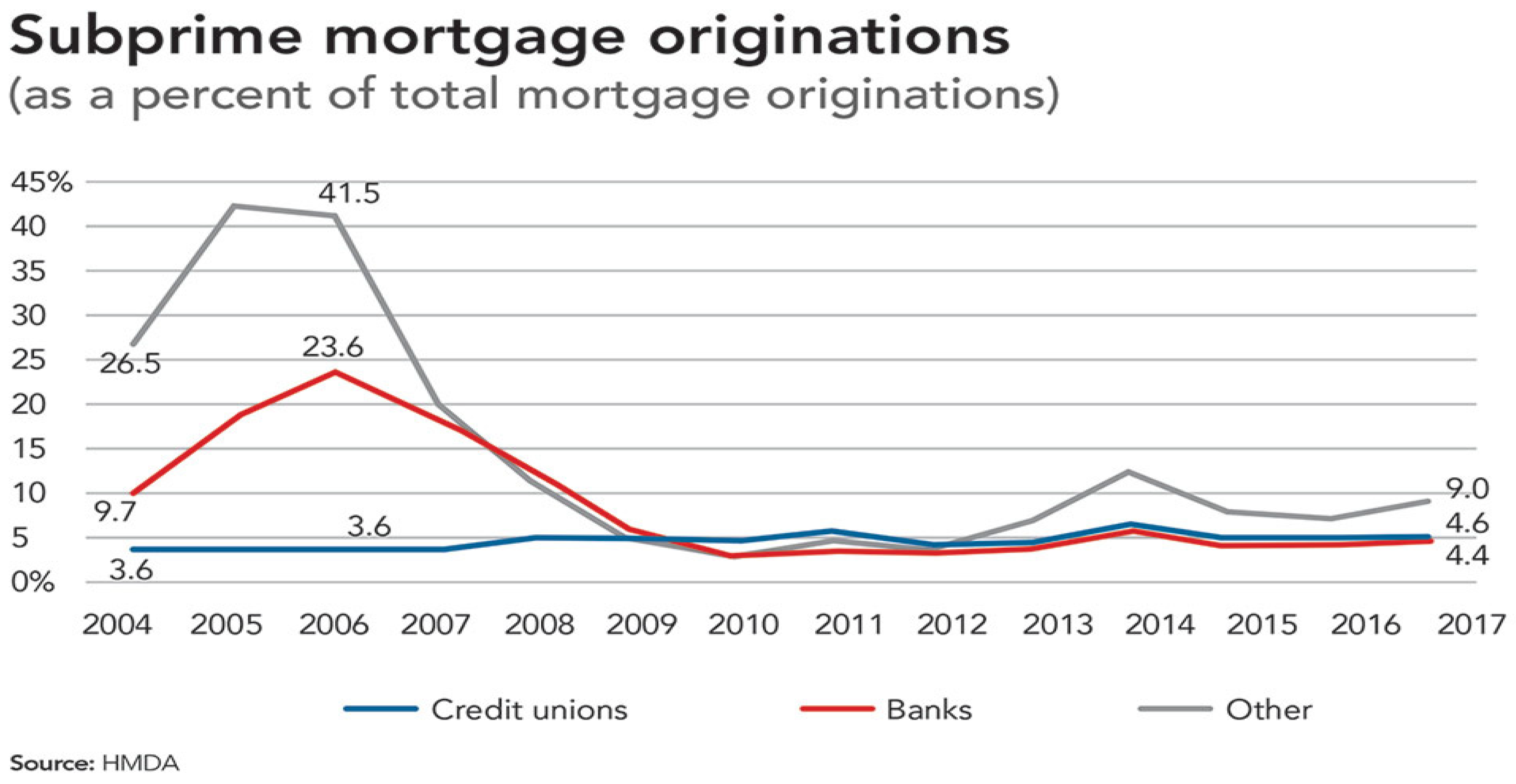
Mortgage-backed non-traditional securities accounted for over 40% of the mortgage market at its peak as reflected in Figure 4; this rate has since been less than10% (8% historical average), with traditional government lenders such as GNMA and Freddie Mac accounting for close to 90–95% of real estate financing. According to data from Inside Mortgage Finance and Urban Institute, this rate is less than 5% today.
Table 1 illustrates the effects of the new stringent underwriting requirements introduced by Dodd–Frank legislation. Home mortgages have become more difficult to obtain resulting in a drastic decrease in mortgage availability. In the 2004–2006 period, there were no down payment requirements, no need for income verification, no debt-to-income ratio requirements and an influx to adjustable-rate mortgages due to the attractive initial “teaser rates”. Today, the no down payment opportunity does not exist, proof of income for a two year-period is required and the most stringent test is the debt-to-income celling of 45%; this ratio assures that a mortgage is based on a financial affordability metric which measures whether the lender will be able to repay the debt. The widespread use of the adjustable-rate mortgage product (greater than 90% of the loans), which was arguably the major culprit of the 2004–2009 housing boom and resulting crisis, is now in check (less than 4%) as lending requirements are now based on the individual’s ability to pay the loan on the highest possible adjustable-reset mortgage rate; this payment amount is substantially higher than an interest-only payment option which was so popular in the 2004–2006 period.
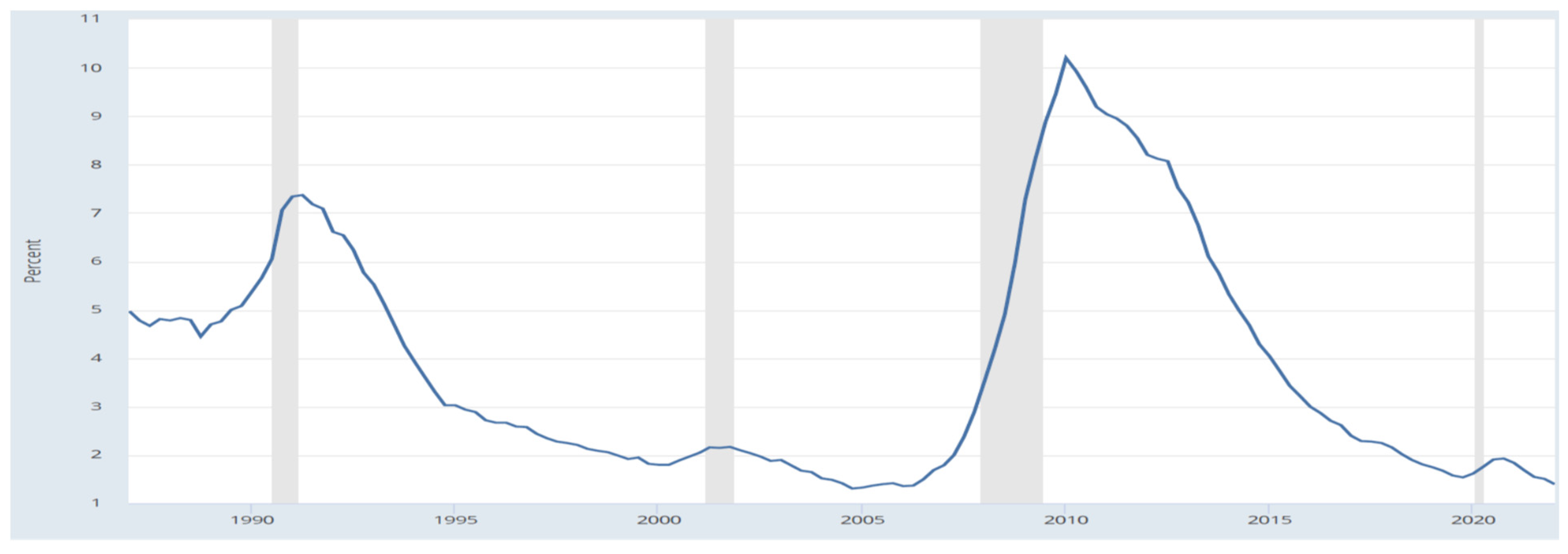
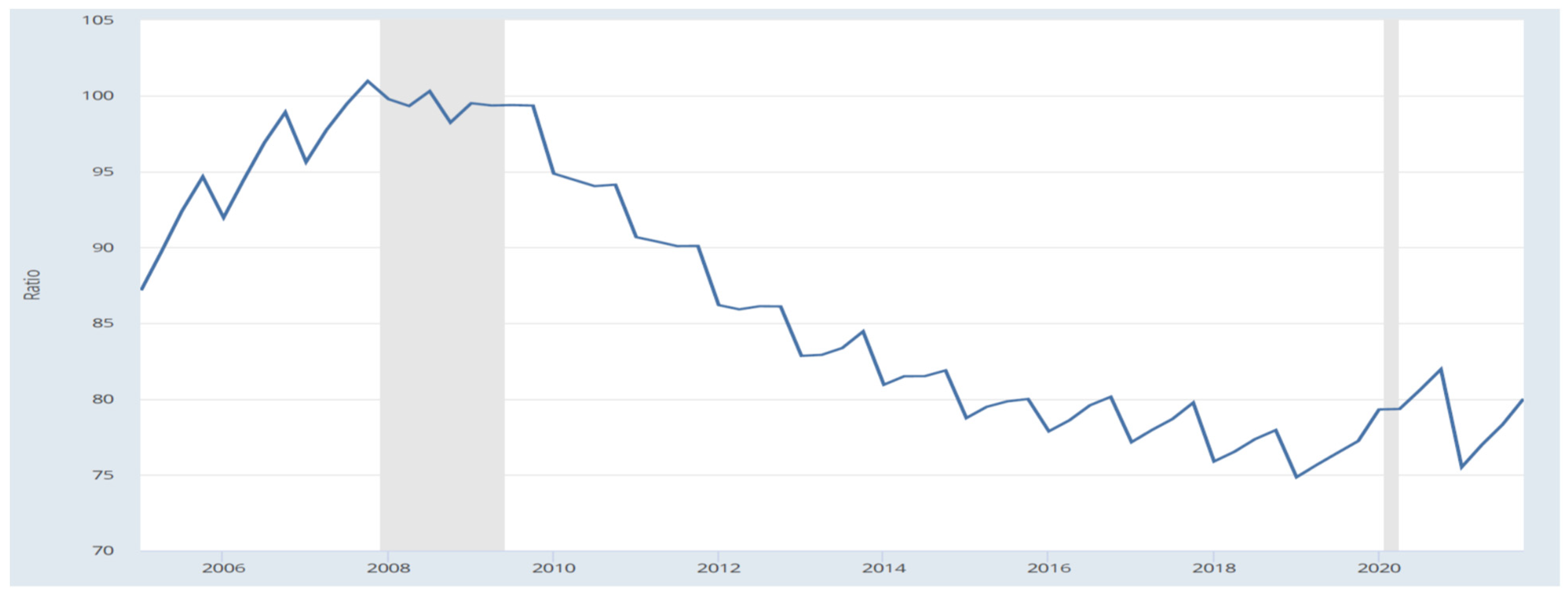
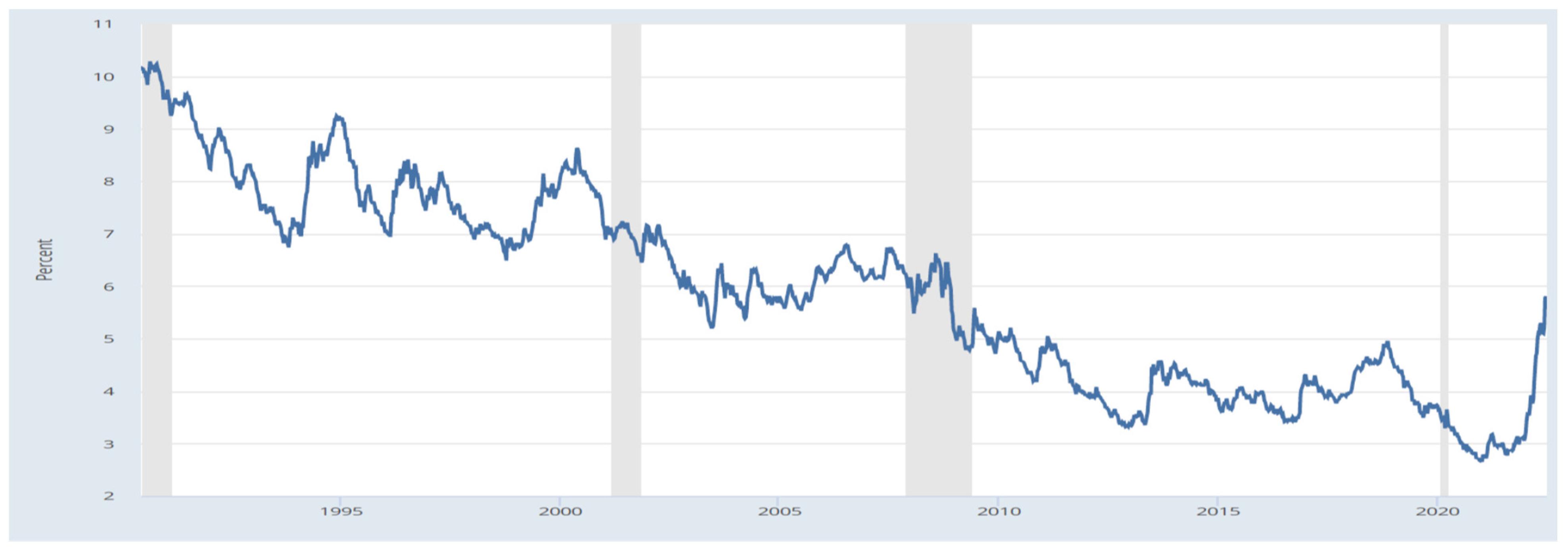
Figure 5 illustrates the delinquency rates on homes secured by mortgages from 1990 to present. We observe a significantly increasing delinquency rate of less than 2% in 2005–2006 to a higher than 10% rate in 2010; this rate has been decreasing steadily and materially post the passage of The Dodd’s-Frank Act. In 2021 and 2022, the delinquency rate is below 1.5% and at a historical low of 1.3% in the most recent first quarter of 2022.
Finally, the Volcker rule, the Federal Reserve “stress test” legislation and The Basel III Accord stringent capital requirements have effectively eliminated major speculative type investing by the banking industry as was prevalent in 2004–2006. Table 2 illustrates the increase in the capital ratios as a result of this regulation for the banking sector. The common equity tier 1 capital ratio increased from 2.5 of 4.5 percent, the tier 1 capital ratio also increased by 2 percentage points from 4 to 6%, while the capital ratio increased to 8%. The introduction of a new ratio called the liquidity ratio was enacted and set at a minimum rate of 4%; this ensures the investment in an adequate amount of liquid, risk-free and easy to sell marketable securities. To further ensure a proper amount of capital as a result of an entity’s “stress test “evaluation, there was a creation of a capital conservation buffer (CCB), requiring financial institutions to retain earnings if their capital is less than 2.5% above the minimum ratios, thereby bringing the total common equity tier 1 minimum requirement to 7%. Large bank holding companies (too large to fail entities) face an additional surcharge to offset the added systematic risk associated with these sized entities and must also meet a total loss-absorbing capacity (TLAC) threshold, where they must meet a minimum ratio of equity to long-term debt. The TLAC is a further buffer of protection to depositors and the FDIC.
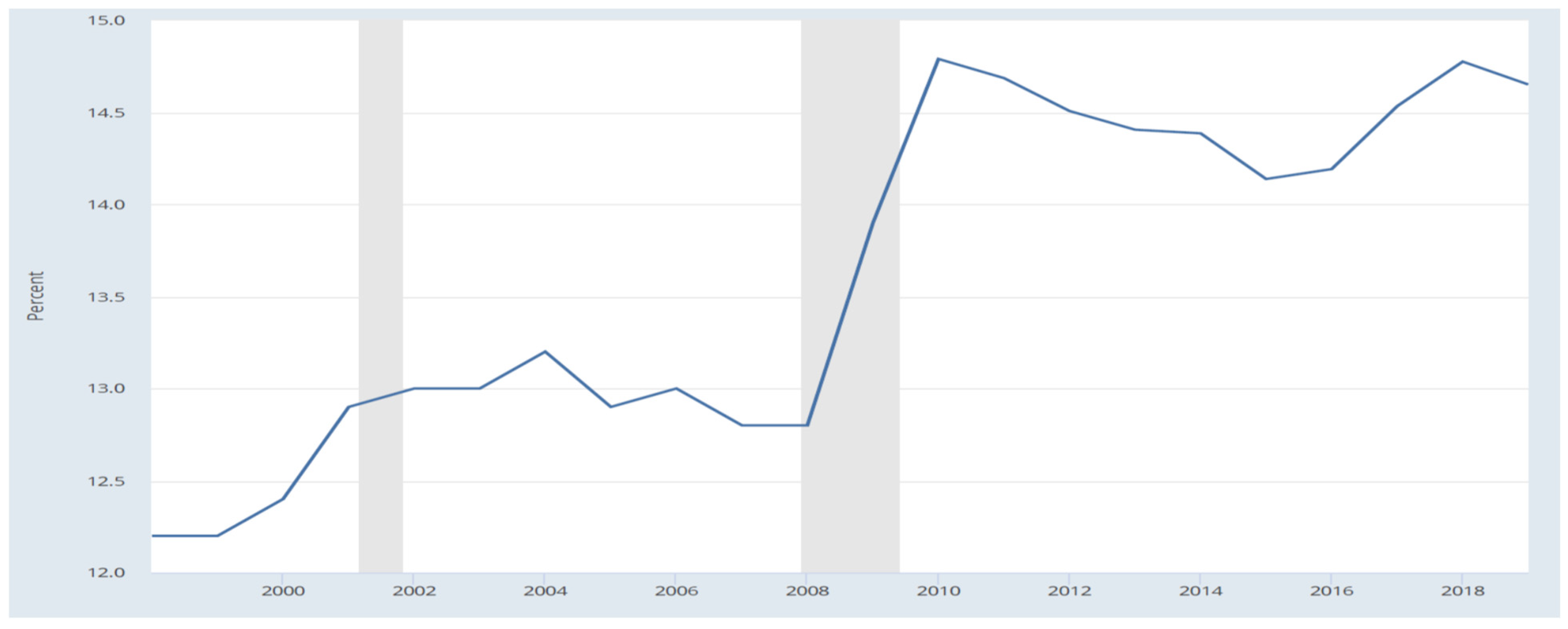
The result is a more economic stable banking sector who must seek a going concern philosophy by the implementation of effective and functioning internal controls, which limit loan issuances and investment purchases of subprime mortgages. Internal control requirements are governed under the Sarbanes-Oxley Act of 2002. Figure 6 reflects the positive effects of Basel III showing an increase in the ratio of banks regulatory capital as a percentage of its risk-weighted assets (RWA).
4. COVID-19 and the Housing Market
COVID-19 turned the US housing market even hotter as the frenzied market pushed prices to record highs. As shown in Figure 1, real home prices after bottoming out in 2011 rose cumulatively by 38.3%, or at an average annual rate of 8.5%, through 2019 prior to the pandemic. When COVID-19 hit the US economy in 2019, housing prices exploded rising cumulatively in real terms by 24.8%, or at a 10.9% annual rate, through the end of 2021. By the end of 2021, real housing prices hit an all-time high, 4.5% above the 2006 high.
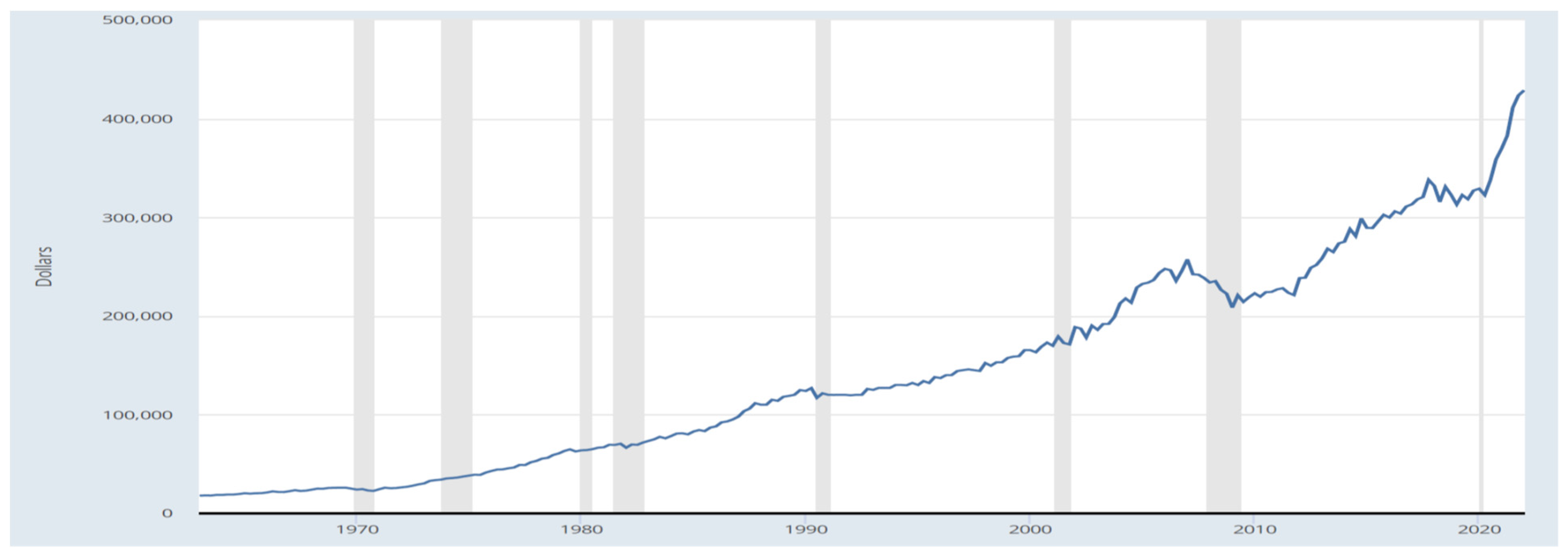
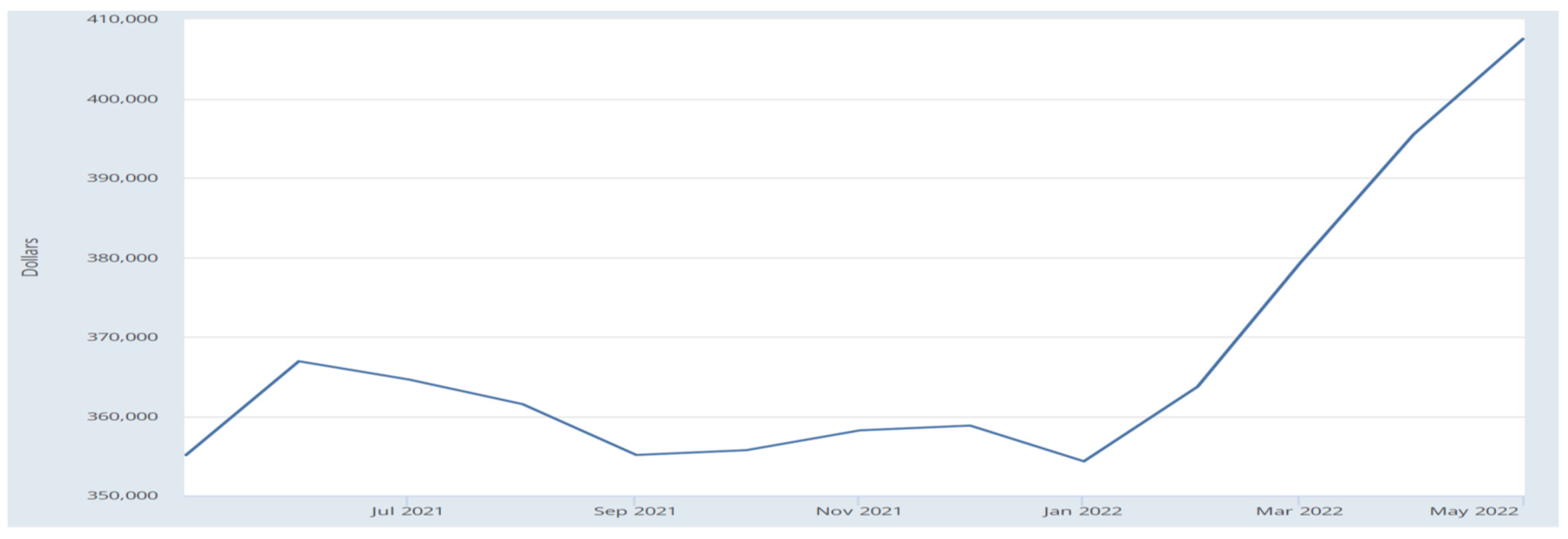
Looking at other housing measures, during the pandemic prices rose sharply for both new and existing homes. As shown in Figure 7, prices of new homes (nominal dollars) rose by 12.8% and 17.6% in 2020 and 2021, respectively. Nationwide, new home prices reached an average price of USD 429,800 in the first quarter of 2022 representing a year-over-year increase of 21.4%. In comparison, the median price of a new home was USD 242,108 in 2012. Shortages of building materials and rising high labor costs continue to put upward pressure on new home prices. Median prices for existing homes (Figure 8) rose by an astounding 30 percent year-over-year in the first quarter of 2022 reaching a level of USD 391,200; these developments have raised concerns of a possible new housing bubble.
Research by Hansen et al. (2022) provides evidence of explosive house price increases during the COVID-19 pandemic and reports that the price pressures in low-density metropolitan areas has been at least equally strong as in high-density metropolitan areas; this data reveals that this finding wasn’t true pre-pandemic. Many people left metropolitan areas during the pandemic and migrated to smaller cities (Haslag and Weagley 2022) causing a reduction in demand for housing in areas with high population density (Liu and Su 2021). The pandemic caused an increase in demand for housing for different reasons than the previous housing increases.
The question is: what distinguishes the current market from that of 2007–2009? There are a number of stark differences between the current housing market and the housing bubble that occurred 15 years ago; these can be grouped into three categories; lending and balance sheet factors, demand side factors and supply side factors and are examined below.
4.1. Lending and Balance Sheet Factors
As discussed earlier, mortgage lending is much more conservative and both households and mortgage lenders are much stronger financially in the COVID-19 period compared to the 2007–2009 housing bubble. Table 1 provides a summary of changes in mortgage requirements. The improvement in the consumer’s balance is evident in Figure 9 which shows that household debt as a share of GDP has fallen sharply since the 2007–2009 recession. In addition, household debt service payments are at their lowest levels since the early 1960s.
4.2. Demand Side Factors
The pandemic triggered a structural shift in the demand for housing as households sought more space for working remotely as well as home entertainment. The affordability migration to the suburbs and Sun Belt markets has left buyers flush with cash from selling homes in higher-priced markets and caused them to bid aggressively for the limited inventory of homes available in lower-priced markets; this is especially true in the South, which has seen a surge in sales of homes priced above USD 500,000. Two other demand side factors have played a significant role.
First, after years of delaying home purchases, millennials, the so-called Generation Rent, emerged as a key driver of demand. Millennials are typically defined as those born between 1981 and 1996 and make up the largest demographic group in US; they represent the fastest-growing segment of home buyers and based on data from NAR accounted for about 37% and 43% of sales in 2020 and 2021, respectively. More millennials will reach the age of 32, the median age for first-time buyers, over the next two years than ever before; this surge in demographic demand from Millennials will drive the housing market for at least the next 5 years.
Second, perhaps the biggest difference between the housing market during the COVID-19 period and the 2007–2009 bubble period is the participation of institutional investors; these investors include private equity firms, mutual fund companies, REITs and pension funds; this has resulted in a structural shift in home buying away from individuals to institutional investors as investors account for a growing share of home purchases; these investors buy single-family homes and apartments and convert them to rental properties; these properties are used to generate income and act as inflation hedges. Investors typically bid aggressively for homes and apartments and in many cases lock out other buyers. Many institutional investors now offer the buy-to-rent investment funds for their clients and consider this a new asset class; this enables the client investors the opportunity to further diversify their investment portfolios and receive steady rental income.
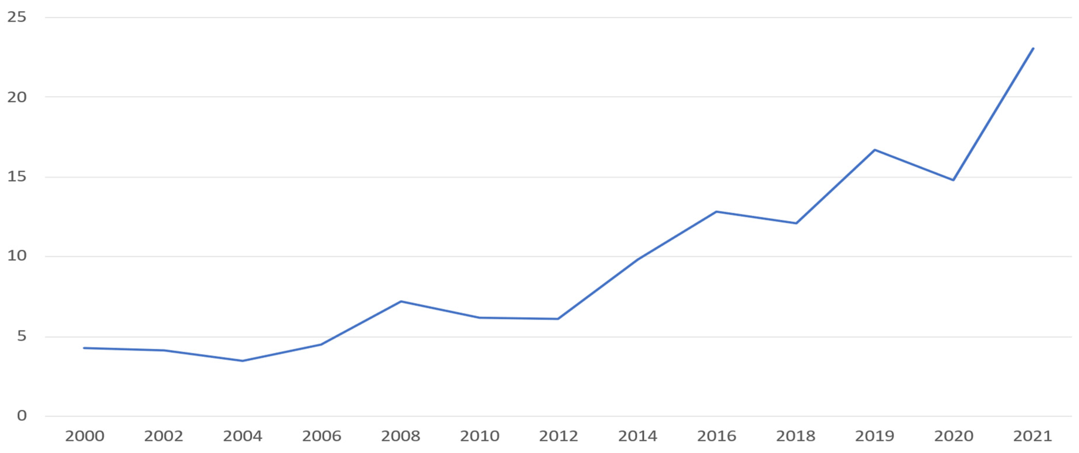
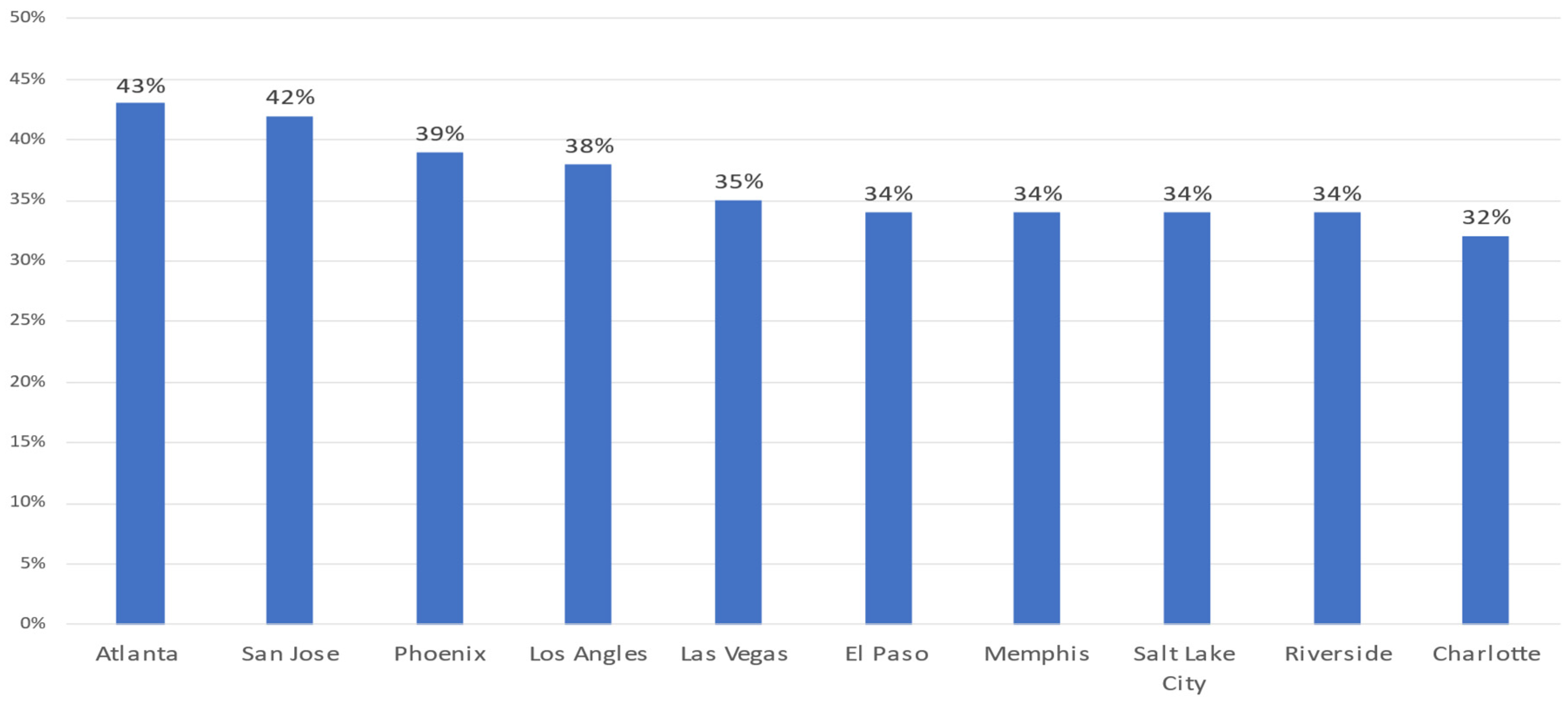
The significance of investor home buying activity is evident in Figure 10. In 2021, investors purchases accounted for almost a quarter of all sales. The investor share of home purchases has increased significantly over the last decade with its share quadrupling from a 6% share in 2012. Homes for rent have become an attractive investment vehicle for income-oriented investors. Investor activity (see Figure 11) has been particularly important in Sun Belt metros, such as Atlanta, Charlotte, Jacksonville and Phoenix and in California. For example, in Atlanta during the third quarter of 2021, investor purchases represented 43% of all home sales. The growing role of investors and changing structure of the demand side of the housing market is important for policy makers since it makes home sales less sensitive to higher home prices; this is because rising home prices, while less attractive to individuals, remain quite attractive to investors as long as rents continue to move higher; furthermore, investor buyers are likely to be less impacted by higher mortgage rates since they can raise funds from various sources and their cost of funds tends to be much lower.
The question that arises is whether the growing buy-to-rent market will cause systemic problems in the financial markets similar to those resulting from the collapse of the subprime market during the housing bubble. Another issue is whether the buy-to-rent model is a way institutional investors are circumventing the financial regulatory structure imposed since the financial crisis. Our view is that there are significant differences between the current buying by institutional investors and the subprime and Alt-A lending that occurred prior to the 2007–2009 financial crisis.
Individuals purchasing homes with subprime and Alt-A mortgages prior to the financial crisis were highly leveraged, vulnerable to rising interest rates and had no incentive to stay in the home if their finances deteriorated (effective put option to borrower if mortgages goes underwater). In contrast, the institutional investor typically buys homes with all-cash offers and doesn’t use mortgage financing at all; they have easy access to capital, raise their funds by issuing shares to individual investors and are highly regulated and subject to fiduciary requirements. Their investment objective is to create large portfolios of rental properties and are motivated by the steady rental income from the homes rather than short-term returns from housing price appreciation. There is little resulting leverage in the system, rising rates have only minimal impacts and there is no incentive to foreclose. As a result, the systemic negative impact of the growing buy-to-rent market on the macro economy is likely to be small; this risk is further mitigated by the national shortage of rental properties, which is only likely to get worse given current building trends.
4.3. Supply Side Factors
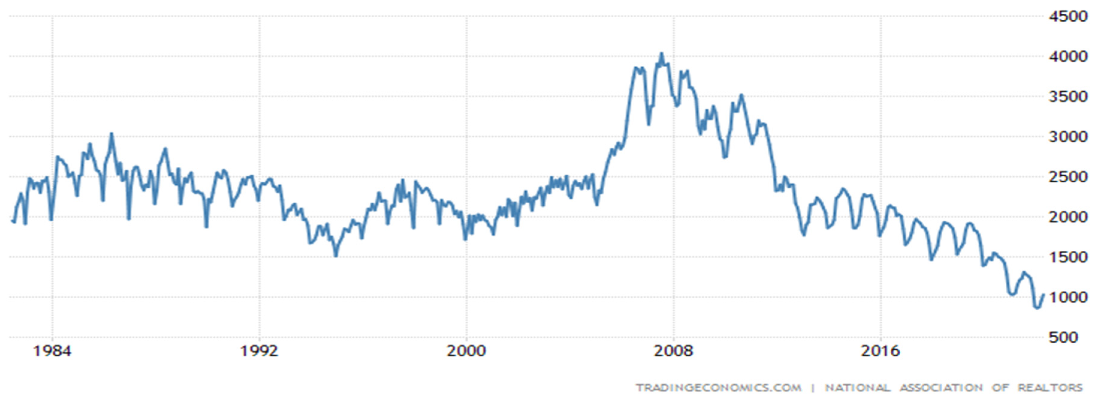
Another significant change in the housing market from the 2007 to 2009 period is on the supply side. Supply conditions during the current cycle are exceedingly tight due to a lack of inventory and shortage of homes available for sale. The implication is that rising rates may not slow homebuilding activity and reduce home prices as typically occurred during past Fed tightening cycles. As shown in Figure 12, the number of single-family and condos units available for sale has been declining since 2007 reaching record lows in 2022. Even before the pandemic, supply conditions in the US housing market were tight and were trending lower.
In 2019, there were roughly 1.6 million existing homes for sale across the country, the equivalent of 3.5 months’ supply at the existing sales pace – both indicators being at low levels relative to history. There were nearly 4 million units available for sale in 2007 (a lot of homes put on market during housing bubble to avoid further price losses) and an average level of 2.8 million and 2.4 million in the decade of the 1980s and 1990s, respectively. Supply shrank further over the course of the pandemic, falling to less than a million homes for sale (or under a 2-month supply at the current sales rate)—the lowest level on record. What explains this downward trend in housing supply? Two major long-term factors are impacting the supply side of the housing market: the declining household mobility rate and the underinvestment in housing.
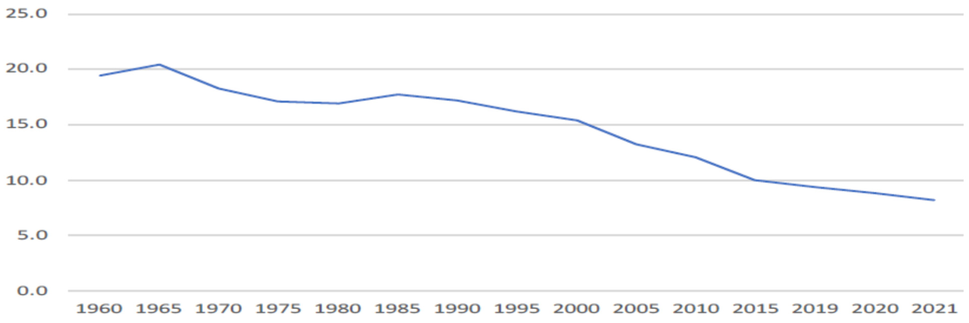
Housing supply is increasingly being limited due to the fact that homeowners are increasingly deciding to stay put and not placing their homes on the market. Geographic mobility measures the rate (percent of population) at which Americans move annually. Most of these moves occur in the same county. Figure 13 shows that geographic mobility has been falling since the mid-1960s with rate of decline accelerating over the last two decades. Mobility declined from nearly 17.0 % in 1980 to a little over 8 % in 2021; this staggering drop in mobility is a problem for the overall economy and the housing market in particular. Workers are unable to move to find new jobs and homeowners are unable to find homes they need to match their changing lifestyle. Every person who doesn’t move clogs the market for others.
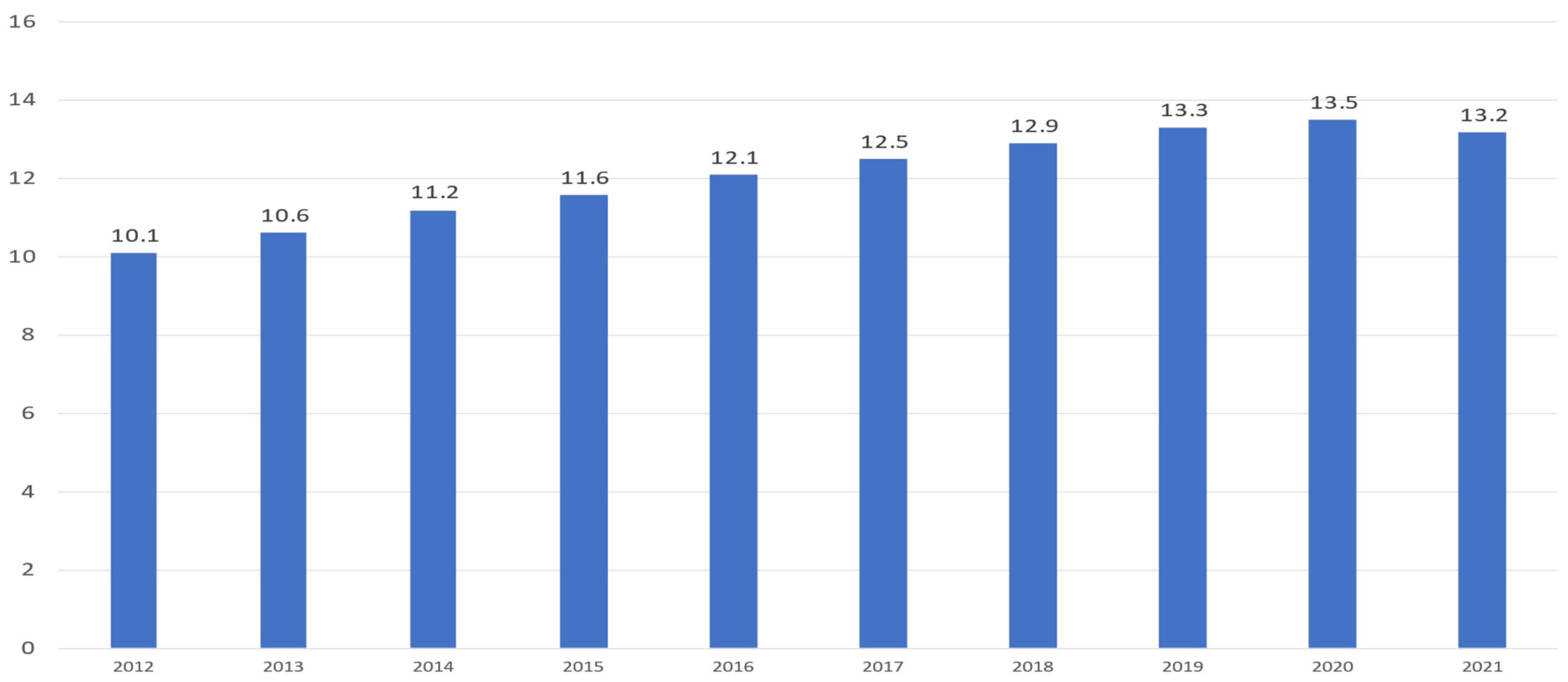
An alternative measure of geographic mobility is provided by Redfin (Figure 14) which shows that homeownership tenure is rising since 2012. Median homeownership tenure rose from 10.1 years in 2012 to 13.5 years in 2020 before dipping slightly in 2021. Americans are living in their homes longer than before, and thus limiting the supply of homes. The rising homeownership tenure and the declining mobility contribute to the housing supply shortages. The pandemic has accentuated the trend since mortgage rates fell to a modern low early in the pandemic; this encouraged a wave of refinancing as homeowners took advantage of the bargain. Now with mortgage rates rising, those bargain rates will have the effect of locking homeowners in place if mortgage rates remain at elevated levels.
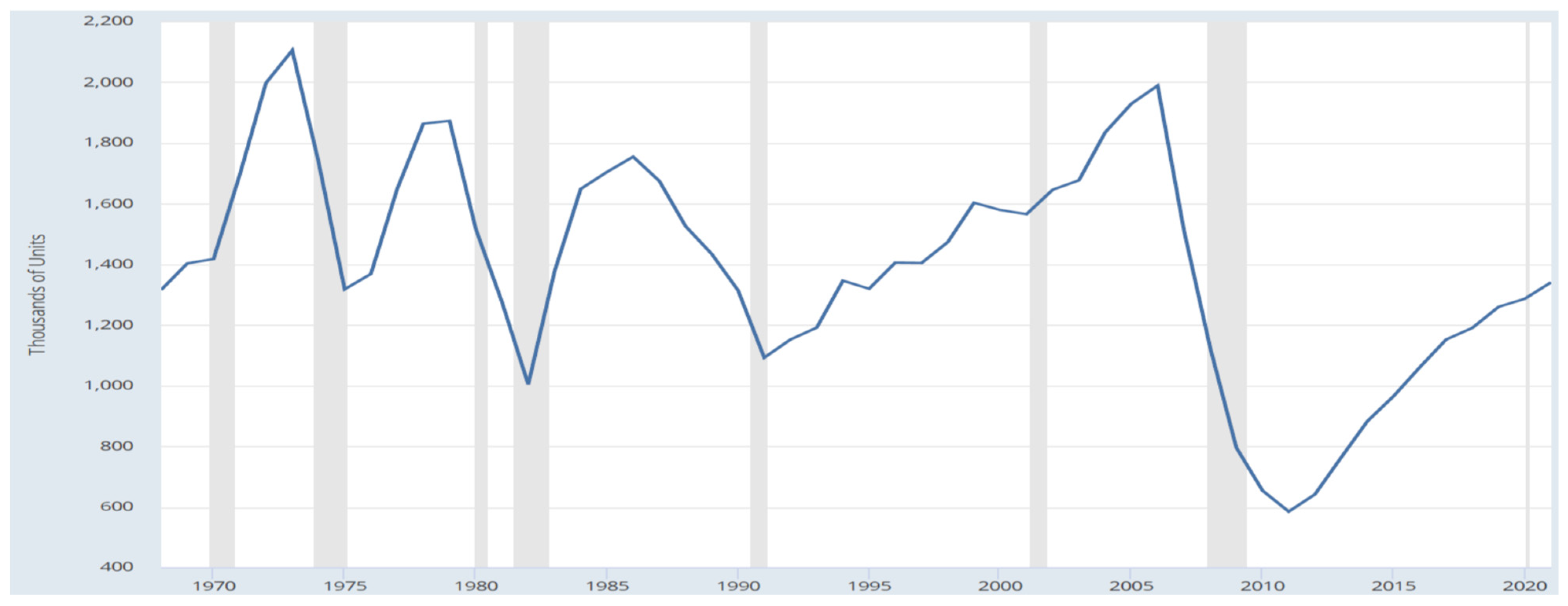
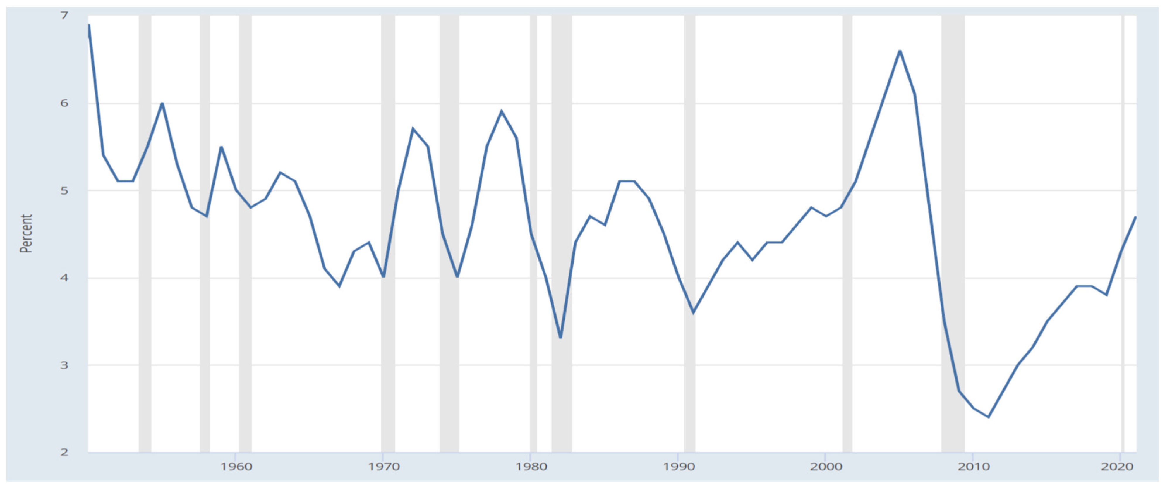
Another factor contributing to the severe housing shortage is the persistent underproduction of housing during the last decade. Figure 15 provides data on the number of homes annually completed in the US. From 1968 through 2005, the annual number of new housing units completed in the United States averaged 1.525 million units; this changed dramatically from 2008 to 2021 when housing completion in the U.S. declined sharply and averaged only 975,000 new unit annually. Even after a considerable increase in construction activity, completions reached a level slightly above 1.3 million units in 2021 which was still well below the historic average. The underinvestment in housing is likewise evident in the data on residential investment as a percent of GDP shown in Figure 16. Since 2008, residential investment as a share of GDP averaged 3.7%; this compares with a 5.1% average in the period 1968 to 2005. Residential investment averaged nearly 6% of GDP in the 1950s and early 1960s.
The underproduction since 2008 has resulted in cumulative shortage of homes. We can get a rough estimate of the underinvestment gap by comparing the historical trend in home completions from 1968 to 2005 (baseline) to the current trend in completions for 2008–2021. In other words, had the 1968 to 2005 trend continued through 2021 how many more homes would have been built; this assumes that the 1968 to 2005 period represents a normal construction period. Based on these trends, we estimate the cumulative underbuilding gap for the 2008 to 2021 period to be over 7.9 million units (see Table 3). The housing market dynamics were quite different in 2007–2009 when if anything there was an excess supply of homes after a surge in construction occurred between 2003 and 2006.
An alternative way to estimate the housing gap is to relate it to the growth in households. To estimate the supply shortfall, one needs to account for the destruction of homes through hurricanes, floods and fire and the demolition/obsolescence of aging homes. Data from the U.S. Department of Housing and Urban Development (HUD) showed that between 2009 and 2017 the U.S. housing stock permanently lost 2.6 million housing units; this translates into an annual average loss of approximately 325,000 units. Using the HUD data and household formation data from the Census, the supply shortfall is estimated in Table 4 by the average annual number of homes completed minus the average annual increase in number of households minus the average annual loss in the housing stock. The household formation approach places the cumulative supply shortfall at almost 4.2 million housing units. A study by Freddie Mac (Khater et al. 2021) estimated the supply gap at 3.8 million units; it should be noted that the supply shortfall of over 4 million units is equivalent to nearly 3 years of current production.
The question of what explains the shortfall in housing supply is a topic for another paper. But essentially it is the result of a confluence of factors, including restrictive zoning and land use laws, lack of buildable land, rising material costs, availability and cost of labor, and NIMBYism.
5. Indicators of a Housing Bubble
As discussed in previous sections, home prices accelerated during the pandemic and are now reaching record levels. The question is whether home prices at these levels are now showing signs of exuberance and if we are now in a real estate bubble. Such bubbles, if they burst, are often followed by severe price declines; this may result in a severe recession as was experienced in 2007–2009. In attempting to identify bubbles before they burst, we can use key indicators to determine whether homes are fairly valued and are justified by economic fundamentals. The idea is to compare current levels of the indicator to historic levels that were previously associated with a housing bubble.
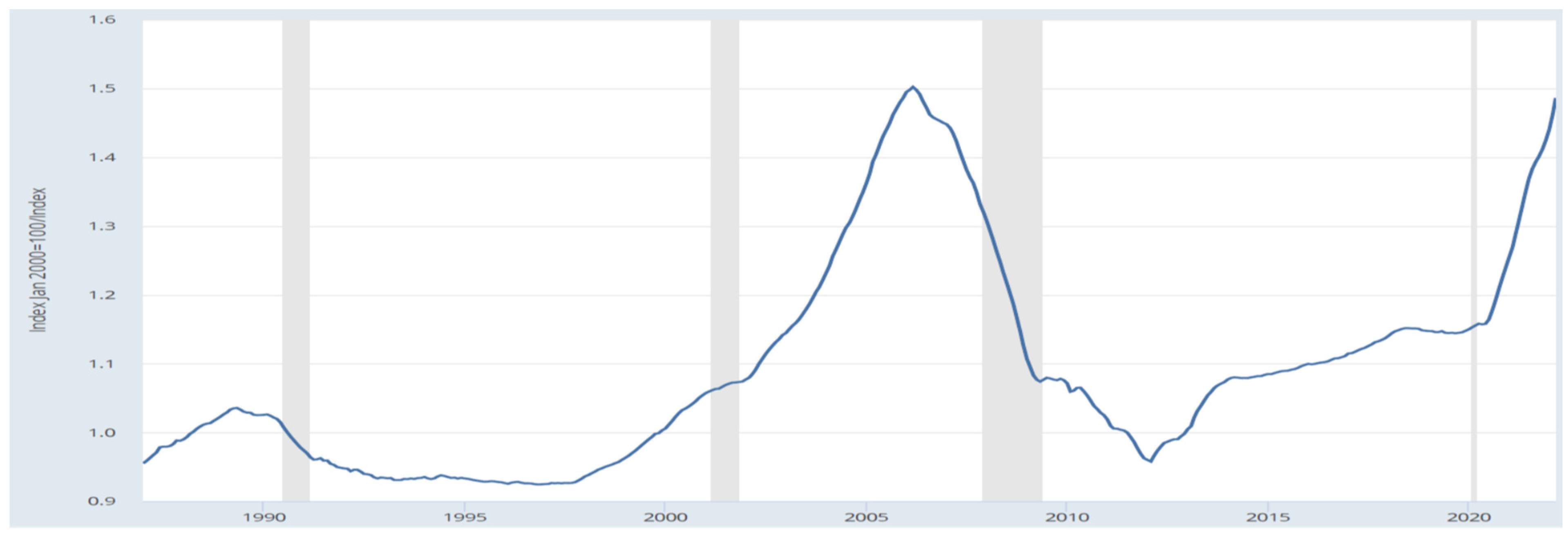
One indictor examining potential troubles in the housing market is the price-to-rent ratio shown in Figure 17; this is a valuation metric and analogous to the price-to-earnings ratio used to value stocks. In this case, the company is the home and dividends are the rents. Historically, the average home price trended around 1 to 1.1 times rent as measured by the CPI-U: Rent of Primary Residence in the US.
During the housing bubble, however, the ratio soared and peaked at around 1.5 in 2006; it then leveled off and returned to its historic trend between 2011 and 2018. What is now of concern is the sharp runup in this ratio over the last 2 years during the pandemic. The move up in the ratio is even sharper than the move that occurred prior to the 2006 peak.
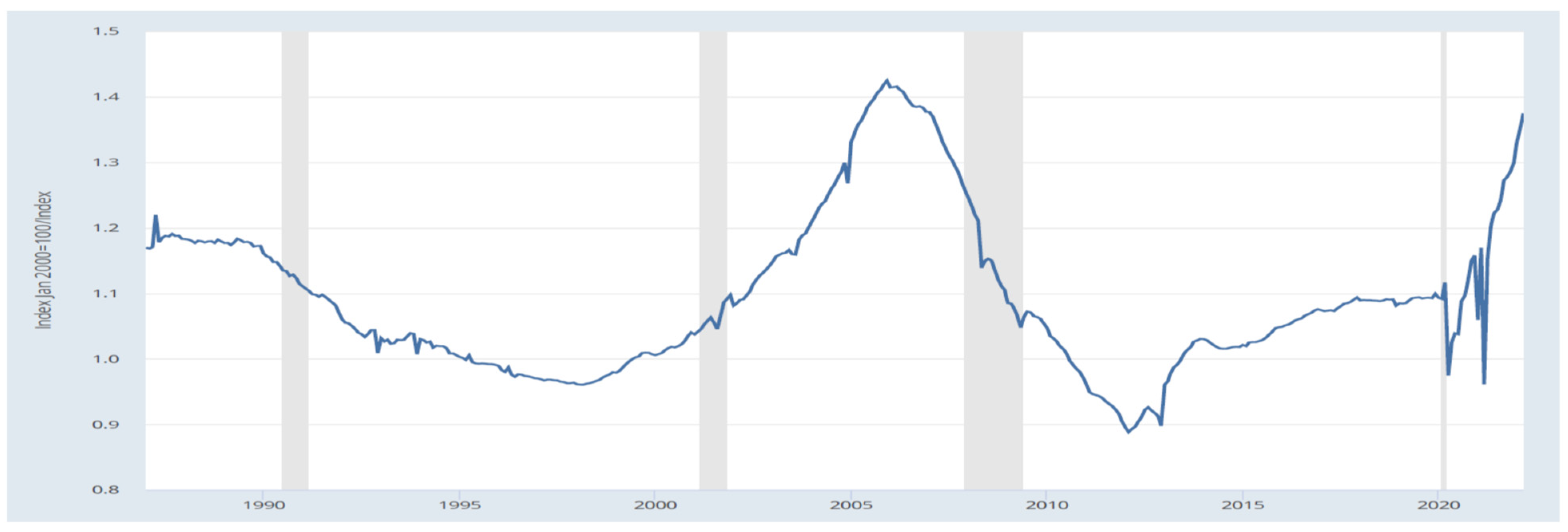
Another important long-term indicator is the price-to-income ratio; this ratio is a measure of housing affordability and is shown in Figure 18. Here, per capita disposable income is used as the indicator of income; this income measure is timely and available monthly in comparison to Census data on household and family income that is available annually and only after a long lag. Like the price-to-rent variable the price-to-income indicator is beginning to flash a yellow warning light. The price-to-income ratio moved up sharply before peaking in 2006 at a level of 1.43; its current reading, as of the first quarter of 2022, is 1.37.
Another indicator of concern is the steep rise in mortgage rates from a historic low of less than 3% in 2020 to close to 6% in early 2022. Higher mortgage rates will likely slow the housing market and encourage the use of adjustable-rate mortgage loans and other mortgage products. The mortgage rate, shown in Figure 19, is still relatively low and still substantially below levels that occurred in the 1990s and the 2000s. The current increase in interest rates will have a moderate effect on housing prices given the supply and demand fundamentals evident in the market.
In summary, the housing market is increasingly showing signs of growing exuberance and potential overvaluation, and as such, needs to be closely monitored by policymakers. Despite these warning signs, housing prices are likely to remain high given the housing market fundamentals.
6. Conclusions
Housing prices surged during the COVID-19 pandemic reaching record levels, raising concern of a housing-related recession similar to that of 2007 to 2009. The rapid home price increases in the period prior to the Great Recession occurred for a number of reasons including: (a) subprime lending; (b) lack of underwriting requirements for mortgages; (c) excessive speculation in mortgage securities; (d) exaggerated credit ratings and (e) lack of regulatory oversight. What is important to understand is that the factors underlying the COVID-19 housing boom are much different from those that drove the housing boom in the period prior to the Great Recession. The major differences are (1) changes in Legislation and (2) Supply and Demand fundamentals.
(1) At the forefront of the differences is the passage of major legislation, which includes: (a) The Dodd–Frank Act, (b) The Basel III Accord and (c) Federal Reserve “stress test” regulations.
The Dodd–Frank Act, which is the most significant and comprehensive of all legislation, significantly lowers the risk on mortgage products by eliminating the no down payment loan option while tightening the underwriting criteria for mortgages based on the borrowers’ ability to pay; it also places various layers of legal responsibility on the lender, which includes comprehensive disclosure about the loan enabling the borrower to understand the major terms of the mortgage. Dodd–Frank also placed more accountability on the credit agencies to provide “realistic and true” ratings. The Volcker rule, which was enacted as part of Dodd–Frank, is aimed in limiting the degree of speculative investments that financial institutions may legally undertake in the goal of preventing “too big to fail” and limiting systemic risk in the financial markets.
In conjunction to placing more fiscal responsibility on financial institutions, the Federal Reserve passed a number of “stress test “regulations along with adherence to The Basel III Accord; these regulations significantly increased minimum capital ratio requirements on financial institutions and created new capital requirements such as leverage, while imposing additional buffer reserves to accommodate potential catastrophes that may occur to a particular financial entity; furthermore critical is the implementation of risk-weighted assets (RWA) capital ratios where capital ratios adjust accordingly on the inherent risk of a bank’s portfolio. Finally, the implementation of Accounting Standards Codification (ASC) 820, requires securities to be priced and presented at a much more conservative “exit price” value which is based on market participants and not internal assumptions. ASC 820 also adds transparency requirements as to the makeup and valuation assumptions of bank owned (and owed)) securities. The passage of this comprehensive and extensive legislation is aimed to best insulate the US from a repeat of a 2007–2009 type financial crisis. As a result, banks are now more capitalized and better able to manage financial stress that could arise from an economic downturn.
(2) Our research attributes the current housing price boom to supply and demand fundamentals.
On the demand side, the price increases are due to an increase in demand (a) from millennials who are entering the housing market in robust numbers, and (b) the significant increase in institutional investor activity in the housing market.
On the supply side, the price increases are due to a decrease in the supply of housing units because of (a) the reduction in geographic mobility, (b) an increase in homeownership tenure and (c) an increasing underproduction in housing units since 2008. Our study estimates that the cumulative underbuilding gap for the 2008–2021 period is between 4.2 million and 7.9 million units. How to increase the supply of housing is a major public policy issue that needs addressing.
While prices in the COVID-19 housing market are at record highs, the improved regulatory structure and the supply and demand fundamentals indicate that a repeat of the 2007–2009 housing crisis is unlikely.
Author Contributions
Conceptualization, P.H., and P.K.; methodology, D.A.; software, D.A.; validation, P.H., D.A., and P.K.; formal analysis, P.K.; investigation, P.H.; resources, P.H.; data curation, D.A.; writing—original draft preparation, P.H.; writing—review and editing, P.K.; visualization, P.H.; supervision, P.K.; project administration, P.H.; funding acquisition, D.A. All authors have read and agreed to the published version of the manuscript.
Funding
This research received no external funding.
Institutional Review Board Statement
Not Applicable.
Informed Consent Statement
Not Applicable.
Data Availability Statement
Found in References section at end of manuscript.
Conflicts of Interest
The authors declare no conflict of interest.
References
- Akerlof, George A., and Robert J. Shiller. 2009. Animal Spirits: How Human Psychology Drives the Economy, and Why It Matters for Global Capitalism. Princeton: Princeton University Press. [Google Scholar]
- Benmelech, Efraim, and Jennifer Dlugosz. 2009. The Credit Rating Crisis, NBER Working Paper 15045. Available online: https://www.nber.org/chapters/c11794.pdf (accessed on 1 May 2022). [CrossRef]
- Birger, Jon. 2008. The Woman Who Called Wall Street’s Meltdown. Available online: https://money.cnn.com/2008/08/04/magazines/fortune/whitney_feature.fortune/index.htm (accessed on 1 May 2022).
- Brunnermeier, Markus K., and Christian Julliard. 2008. Money Illusion and Housing Frenzies. The Review of Financial Studies 21: 135–80. [Google Scholar] [CrossRef]
- Case, Karl E., and Robert J. Shiller. 1989. The Efficiency of the Market for Single-Family Homes. The American Economic Review 79: 125–37. [Google Scholar]
- Chinco, Alex, and Christopher Mayer. 2016. Misinformed Speculators and Mispricing in the Housing Market. The Review of Financial Studies 29: 486–522. [Google Scholar] [CrossRef]
- Courchane, Marsha J., and Peter M. Zorn. 2012. Differential Access to and pricing of Home Mortgages: 2004 through 2009. Real Estate Economics 40: S115–58. [Google Scholar] [CrossRef]
- Demyanyk, Yuliya, and Otto Van Hemert. 2011. Understanding the Subprime Mortgage Crisis. Review of Financial Studies 24: 1848–80. [Google Scholar] [CrossRef]
- Drozdowski, Grzegorz. 2021. Economic Calculus Qua an Instrument to Support Sustainable Development under Increasing Risk. Journal of Risk and Financial Management 14: 15. [Google Scholar] [CrossRef]
- European Central Bank. 2021. ECB to Stress Test 38 Euro Area Banks as Part of the 2021 EU-Wide Stress Test Led by EBA. Available online: https://www.bankingsupervision.europa.eu/press/pr/date/2021/html/ssm.pr210129~69d2d006ec.en.html (accessed on 1 June 2022).
- Favilukis, Jack, Sydney C. Ludvigson, and Stijn Van Nieuwerburgh. 2010. The Macroeconomic Effects of Housing Wealth, Housing Finance, and Limited Risk-Sharing in General Equilibrium. Working Paper 15988. Cambridge, MA: National Bureau of Economic Research (NBER). [Google Scholar]
- FDIC. 2006. FDIC: Interest Only Mortgage Payments and Option Payments ARMS. Available online: https://www.fdic.gov/consumers/consumer/interest-only/index.html (accessed on 1 July 2022).
- Financial Accounting Standards Board. 2018. Fair Value Measurement Topic 820. No. 2018-13. Norwalk: Financial Accounting Standards Board. [Google Scholar]
- Geanakoplos, John. 2010. Solving the Recent Crisis and Managing the Leverage Cycle. Cowles Foundation Discussion Paper No. 1751. Available online: https://papers.ssrn.com/sol3/papers.cfm?abstract_id=1539488 (accessed on 1 June 2022).
- Glaeser, Edward L., Joseph Gyourko, and Albert Saiz. 2008. Housing Supply and Housing Bubbles. Journal of Urban Economics 64: 198–217. [Google Scholar] [CrossRef] [Green Version]
- Glaeser, Edward L., Joshua D. Gottlieb, and Joseph Gyourko. 2010. Can Cheap Credit Explain the Housing Boom? Working Paper 16230. Cambridge, MA: National Bureau of Economic Research (NBER). [Google Scholar]
- Government Publications. 2011. The Financial Crisis Inquiry Report: Final Report of the National Commission on the Causes of the Financial and Economic Crisis in the United States, Executive Agency Publications, Y 3.2:F 49/2/C 86. Available online: https://www.gpo.gov/fdsys/pkg/GPO-FCIC/content-detail.html (accessed on 1 June 2022).
- Hansen, Jacob H., Stig Vinther Møller, Thomas Quistgaard Pedersen, and Erik Christian Montes Schütte. 2022. House Price Bubbles under the COVID-19 Pandemic. Available online: https://ssrn.com/abstract=4067276 (accessed on 1 May 2022). [CrossRef]
- Haslag, Peter H., and Daniel Weagley. 2022. From L.A. to Boise: How Migration Has Changed during the COVID-19 Pandemic. Available online: https://ssrn.com/abstract=3808326 (accessed on 1 June 2022). [CrossRef]
- Haughwout, Andrew, Donghoon Lee, Joseph Tracy, and Wilbert van der Klaauw. 2011. Real Estate Investors, the Leverage Cycle, and the Housing Market Crisis. Federal Reserve Bank of New York Staff Reports No. 514. Available online: https://papers.ssrn.com/sol3/papers.cfm?abstract_id=1926858 (accessed on 1 June 2022).
- Himmelberg, Charles, Christopher Mayer, and Todd Sinai. 2005. Assessing High House Prices: Bubbles, Fundamentals, and Misperceptions. Journal of Economic Perspectives 19: 67–92. [Google Scholar] [CrossRef] [Green Version]
- Khater, Sam, Len Kiefer, and Venkataramana Yanamanda. 2021. Housing Supply: A Growing Deficit. Freddie Mac Economic & Research Notes, May 7. [Google Scholar]
- Knox, Noelle. 2006. 43% of First-Time Home Buyers Put No Money Down. USA Today. Available online: https://usatoday30.usatoday.com/money/perfi/housing/2006-01-17-real-estate-usat_x.htm (accessed on 1 June 2022).
- Liu, Sitian, and Yichen Su. 2021. The Impact of the COVID-19 Pandemic on the Demand for Density: Evidence from the U.S. Housing Market. Economics Letters 207: 110010. [Google Scholar] [CrossRef] [PubMed]
- Mayer, Christopher. 2011. Housing Bubbles: A Survey. Annual Review of Economics 3: 559–77. [Google Scholar] [CrossRef] [Green Version]
- McCarthy, Jonathan, and Richard W. Peach. 2004. Are Home Prices the Next “Bubble”? FRBNY Economic Policy Review. Available online: https://papers.ssrn.com/sol3/papers.cfm?abstract_id=634265 (accessed on 1 May 2022).
- Mian, Atif, and Amir Sufi. 2009. The Consequences of Mortgage Credit Expansion: Evidence from the US Mortgage Default Crisis. Quarterly Journal of Economics 124: 1449–96. [Google Scholar] [CrossRef]
- Pavlov, Andrey, and Susan M. Wachter. 2006. The Inevitability of Marketwide Underpricing of Mortgage Default Risk. Real Estate Economics 34: 479–96. [Google Scholar] [CrossRef]
- Rajan, Raghuram G. 2006. Has Finance Made the World Riskier? European Financial Management 12: 499–533. [Google Scholar] [CrossRef]
- Shiller, Robert J. 2007. Understanding Recent Trends in House Prices and Home Ownership. NBER Working Paper 13553. Available online: http://www.nber.org/papers/w13553 (accessed on 1 May 2022).
- Simkovic, Michael. 2013. Competition and Crisis in Mortgage Securitization. Indiana Law Journal 88: 4. [Google Scholar] [CrossRef] [Green Version]
- Smith, Elliot B. 2008. Bringing Down Wall Street as Ratings Let Loose Subprime Scourge. Bloomberg Business, September 24. [Google Scholar]
- Stiglitz, Joseph. 1990. Symposium on Bubbles. Journal of Economic Perspectives 4: 13–17. [Google Scholar] [CrossRef] [Green Version]
- Stiglitz, Joseph. 2009. The Anatomy of a Murder: Who Killed America’s Economy? Critical Review 21: 329–39. [Google Scholar] [CrossRef]
- Taylor, John B. 2009. Getting Off Track: How Government Actions and Interventions Caused, Prolonged, and Worsened the Financial Crisis. Stanford: Hoover Institution Press. [Google Scholar]
- The Federal Reserve. n.d. Dodd–Frank Act Stress Test Publications. Available online: https://www.federalreserve.gov/publications/Dodd–Frank-act-stress-test-publications.htm (accessed on 1 July 2022).
- Ward, Judy. 2004. Countrywide Extends its Automated Underwriting System. Bank Systems & Technology, February 6. [Google Scholar]
- Zandi, Mark. 2009. Financial Shock: Global Panic and Government Bailouts—How We Got Here and What Must Be Done to Fix It, 1st ed. Upper Saddle River: FT Press. ISBN 978-013701663-1. [Google Scholar]
Figure 1.
Real Residential Housing Prices in the US. Source: Bank of International Settlements.

Figure 2.
Projected Credit Losses and Rates Annual Loss Rate. Source: Davidson Company Inc.

Figure 3.
Loss Adjusted Coupon Rate. Source: Davidson Company Inc.

Figure 4.
Subprime Mortgage Originations.

Figure 5.
Delinquency Rate on Loans Secured by Real Estate, All Commercial Banks. Source: Board of Governors of the Federal Reserve.
Figure 5.
Delinquency Rate on Loans Secured by Real Estate, All Commercial Banks. Source: Board of Governors of the Federal Reserve.

Figure 6.
Bank Regulatory Capital to Risk-Weighted Assets (RWA). Source: World bank.

Figure 7.
Median Sales Prices for New Homes Sold in US. Source: Census; HUD.

Figure 8.
Median Sales Price of Existing Home. Source: National Association of Realtors.

Figure 9.
Household Debt as a Percent of GDP. Source: International Monetary Fund.

Figure 10.
Home Purchases by Investors (Percent share). Source: Corelogic.

Figure 11.
Highest Investor Share by Metro (Q3 2021). Source: Corelogic, Redfin.

Figure 12.
Total Housing Inventory (number of single-family and condos units available for sale).

Figure 13.
Geographic Mobility Rates (% of population). Source: Current Population Survey.

Figure 14.
Homeowners Tenure (median homeowner tenure in years). Source: Redfin.

Figure 15.
New Privately-Owned Housing Units Completed: Total Units. Source: Census; HUD.

Figure 16.
Residential Investment as a Percent of GDP. Source: US Bureau of Economic Analysis.

Figure 17.
Ratio of S&P Case Shiller Price Index to CPI-U: Rent of Primary Residence in the US. Source: S&P Dow Jones; Labor Department.
Figure 17.
Ratio of S&P Case Shiller Price Index to CPI-U: Rent of Primary Residence in the US. Source: S&P Dow Jones; Labor Department.

Figure 18.
Ratio of S&P Case Shiller Price Index to Per Capita Disposable Income. Source: S&P Dow Jones; Bureau of Economic Analysis.
Figure 18.
Ratio of S&P Case Shiller Price Index to Per Capita Disposable Income. Source: S&P Dow Jones; Bureau of Economic Analysis.

Figure 19.
30 Year Average Fixed Mortgage Rate. Source: Freddie Mac.


Table 1.
Comparison of Mortgage Requirements Between the 2005–2009 and 2019–2022 Periods.
| Minimum Requirement | 2004–2009 | 2019–2022 |
|---|---|---|
| Down Payment | Low or no down payment | 3% of loan |
| Income | Stated Income (no verification) | Proof of Income (past 2 years) |
| Credit Score | Below 620 considered subprime loan | 620 |
| Debt to Income Ratio | No DTI ratio requirement | 45% |
| Adjustable-Rate Mortgages | More than 90% | About 4% |
Table 2.
Minimum Capital Requirements for National Bank or Federal Savings Association.
| A common equity tier 1 capital ratio of 4.5 percent. |
| A tier 1 capital ratio of 6 percent |
| A total capital ratio of 8 percent. |
| A leverage ratio of 4 percent |
| For advanced approaches national banks or Federal savings associations or, for Category III OCC-regulated institutions, a supplementary leverage ratio of 3 percent |
| For Federal savings associations, a tangible capital ratio of 1.5 percent. |
| Additional buffer requirements in various situations |
Table 3.
Supply Shortfall Based on Historic Trends.
| Period | Average Annual Completions |
|---|---|
| 1968–2005 | 1,585,000 |
| 2008–2021 | 975,000 |
| Annual Gap | 610,000 |
| Cumulative Gap for 2008–2021 | 7,930,000 |
Sources: Census, HUD.
Table 4.
Supply Shortfall Based on Household Formations Trends.
| Period | Average Annual Completions | Average Annual Increase in Households | Lost Housing Stock | Annual Supply Shortfall |
|---|---|---|---|---|
| 1968–2005 | 1,585,000 | 1,325,000 | 265,000 * | −5000 |
| 2008–2021 | 975,000 | 972,000 | 325,000 | −322,000 |
| Cumulative Gap for 2008–2021 | −4,186,000 |
* Adjusted for housing stock by Authors. Sources: Census, HUD.
Publisher’s Note: MDPI stays neutral with regard to jurisdictional claims in published maps and institutional affiliations. |
© 2022 by the authors. Licensee MDPI, Basel, Switzerland. This article is an open access article distributed under the terms and conditions of the Creative Commons Attribution (CC BY) license (https://creativecommons.org/licenses/by/4.0/).
Share and Cite
MDPI and ACS Style
Afxentiou, D.; Harris, P.; Kutasovic, P. The COVID-19 Housing Boom: Is a 2007–2009-Type Crisis on the Horizon? J. Risk Financial Manag. 2022, 15, 371. https://doi.org/10.3390/jrfm15080371
AMA Style
Afxentiou D, Harris P, Kutasovic P. The COVID-19 Housing Boom: Is a 2007–2009-Type Crisis on the Horizon? Journal of Risk and Financial Management. 2022; 15(8):371. https://doi.org/10.3390/jrfm15080371
Chicago/Turabian StyleAfxentiou, Diamando, Peter Harris, and Paul Kutasovic. 2022. "The COVID-19 Housing Boom: Is a 2007–2009-Type Crisis on the Horizon?" Journal of Risk and Financial Management 15, no. 8: 371. https://doi.org/10.3390/jrfm15080371