
Causality between Arbitrage and Liquidity in Platinum Futures


1
Graduate School of Economics, Kobe University, 2-1 Rokkodai-cho, Nada, Kobe 657-8501, Japan
2
Faculty of International Liberal Arts, Akita International University, Yuwa, Akita-City 010-1292, Japan
*
Authors to whom correspondence should be addressed.
J. Risk Financial Manag. 2022, 15(12), 593; https://doi.org/10.3390/jrfm15120593
Submission received: 3 November 2022
/
Revised: 30 November 2022
/
Accepted: 2 December 2022
/
Published: 9 December 2022
(This article belongs to the Special Issue Commodity Market Finance)
Abstract
:Arbitrage and liquidity are interrelated. Liquidity facilitates arbitrageurs’ trading on deviations from the law of one price. However, whether arbitrage opportunity leads to an increase or decrease in liquidity depends on the cause of the deviation. A demand shock leads to greater liquidity, while asymmetric information is toxic to liquidity. We examine how arbitrage and liquidity influence each other in the world’s largest platinum futures markets on exchanges in New York and Tokyo. The markets provide an interesting institutional setting because the futures are based on an identical underlying commodity but exhibit different liquidity characteristics both intraday and over their lifespans. Using intraday data, we find that deviation in currency-adjusted futures prices leads, on average, to an immediate increase in liquidity, suggesting that demand shocks are the dominant driver of arbitrage opportunities. Less actively traded futures experience a greater liquidity effect. Arbitrageurs improve liquidity in both New York and Tokyo by acting as discretionary liquidity traders and cross-sectional market-makers.
JEL Classification:
G13; G14; G15; Q021. Introduction
The law of one price (LOOP) suggests that the prices of futures on an identical underlying commodity that are traded on different exchanges should be the same, taking into account the currency of denomination and differences in contract specifications. Deviation in such prices gives rise to an arbitrage opportunity that, in competitive and efficient markets, would lead to prices equalizing across exchanges.
Liquidity has long been thought to influence the ability of market participants to conduct arbitrage in financial markets. High levels of market liquidity allow arbitrageurs to exploit price differences across markets that trade homogeneous, similar or closely linked securities. Low liquidity limits arbitrage, as traders who attempt to profit on the convergence of prices are exposed to higher transactions costs and a greater risk that prices move against their trades. Although in theory arbitrage refers to a riskless opportunity to profit from a pricing discrepancy, in practice, such opportunities are rare. Limits to arbitrage include fundamental risk, noise trader risk and implementation costs. Low liquidity or differences in liquidity between markets may enhance limits to arbitrage.
Recent research has examined how arbitrage may affect liquidity. Theory suggests that arbitrage profit opportunities may either lead to an improvement or a deterioration in liquidity, depending on the nature of the shock that led to the deviation in prices between markets. Arbitrage opportunities that arise due to non-fundamental demand shocks are liquidity-enhancing, as arbitrageurs enter both markets to transact against the direction of the shock (Gromb and Vayanos 2010; Holden 1995). Arbitrage trades are likely to be spread over time to minimise price impact, which would bring about autocorrelated orders and a persistent liquidity effect (Kyle 1985; Roll et al. 2007). Arbitragers trade against prevailing demand to provide liquidity to other market participants in exchange for a premium and, in doing so, improve market integration (Rösch 2021). Under these circumstances, arbitrage profit opportunities would be expected to lead to an increase in liquidity.
Alternatively, arbitrage opportunities that arise due to information asymmetry may reduce liquidity due to adverse selection (Foucault et al. 2017; Kumar and Seppi 1994). So-called toxic arbitrage opportunities occur when new information is incorporated in one market’s price, leading to a short-lived price deviation with respect to the other market (Johannsen 2017). Foucault et al.’s (2017) model suggests dealers respond to toxic arbitrage by widening bid–ask spreads to slow their trading and compensate for the risk of transacting at stale prices. Toxic arbitrage opportunities lead to a decrease in liquidity. Furthermore, limits to arbitrage may dissuade arbitrageurs from taking advantage of price deviations. For instance, arbitrageurs may avoid arbitrage trades with high idiosyncratic volatility that would expose them to losses or the need to liquidate the arbitrage trade (Shleifer and Vishny 1997).
These different strands of the literature raise several empirical questions. What is the direction of causality between arbitrage and liquidity? Are arbitrage opportunities generally associated with lower or higher liquidity? Does the sign and magnitude of the relationship between arbitrage and liquidity change when a futures contract is in a more or less actively traded phase of its lifespan?
Researchers have examined the empirical relationship between arbitrage and liquidity for similar or related securities in equity, currency and fixed-income markets. Roll et al. (2007) find bidirectional relationships between liquidity on the New York Stock Exchange (NYSE) and arbitrage opportunities in the futures cash basis associated with the NYSE composite index futures contract. Schultz and Shive (2010) show that arbitrage opportunities between dual-class shares, which are typically driven by the more liquid share, lead to increased trade volumes, with trades within one or the other share class being relatively more important in closing the price gap than matched trades across the dual-share classes. Marshall et al. (2013a) examines arbitrage opportunities in similar highly liquid exchange traded funds (ETFs) that track the S&P500 index. Their results suggest that a fall in liquidity combined with an increase in liquidity risk contribute to arbitrage opportunities, which are rapidly eliminated with buyer (seller)-initiated trades in the underpriced (overpriced) ETF that is most prevalent. Ghadhab (2018) find that arbitrage opportunities in cross-listed stocks lead to greater liquidity. Rösch (2021) examine the arbitrage and liquidity relationships between the American Depositary Receipt (ADR) market and home market shares and find that a positive shock to arbitrage decreased the price deviations and bid–ask spreads. Rappoport and Tuzun (2020) find bidirectional Granger causality between liquidity and arbitrage opportunity between ETFs and their constituents in both equity and bond markets, but the effect of arbitrage on liquidity and vice versa is larger for bond than equity markets, as bond ETF constituents are generally less actively traded. Foucault et al. (2017) examine triangular arbitrage in foreign exchange markets and find a positive relationship between illiquidity and both the fraction of toxic arbitrage opportunities and arbitrageurs’ relative speed in trading.
Several recently published articles analyze commodity futures, including the platinum contract traded in New York. Ludwig (2019) investigate the relationship between speculative activity and liquidity, while Bohl et al. (2021) consider speculative activity and informational efficiency. Lauter and Prokopczuk (2022) identify low-frequency proxies for commodity futures market quality. Boos and Grob (2022) investigate the trading strategies of managed futures funds, Sakkas and Tessaromatis (2020) evaluate factor-based commodity futures investment, and Kwon et al. (2020) evaluate model momentum. Sun et al. (2023) examine the price impact of traders on commodity futures. Tokyo platinum contracts also feature in recent published research. Boubaker et al. (2021) evaluate the performance of momentum based on functional data analysis. Iwatsubo and Watkins (2020) present evidence on which traders influence the efficient prices of commodity futures traded in Tokyo. Iwatsubo et al. (2018) examine the intraday seasonality of the microstructure characteristics in the platinum and gold futures contracts traded in New York and Tokyo.
To our knowledge, there is no published research on the potentially bidirectional causal relationship between arbitrage and liquidity in commodity futures markets. However, the arbitrage–liquidity relationship is particularly relevant for commodity futures, given their institutional environment. It is now common for multiple futures exchanges to list contracts based on the same underlying commodity traded in concurrent or overlapping sessions in different countries. Exchanges use day and night trading sessions to facilitate market access by participants in different time zones around the world, arguably to boost liquidity and promote efficient price discovery. Arbitrageurs can trade on LOOP violations between exchanges around the clock. With sufficient liquidity, arbitrage activity between the exchanges is expected to encourage a single world price for futures based on an identical underlying commodity, consistent with the LOOP after adjusting for contract specifications and exchange rates. Hence, understanding the potentially bidirectional relationship between arbitrage and liquidity, and particularly whether arbitrage is beneficial or harmful for liquidity, is of practical importance in commodity futures markets. Our research contributes toward filling this gap in the literature.
In this paper, we examine the relationship between arbitrage and liquidity in the platinum futures markets on the New York Mercantile Exchange (NYMEX) and the Tokyo Commodity Exchange (TOCOM), taking into account both potential directions of causality. We use intraday price and volume data for one contract on each exchange with a common expiry month. The platinum futures markets in New York and Tokyo provide an interesting environment to examine the interaction of arbitrage and liquidity. The exchanges are the primary global derivative venues for hedging and speculation in platinum. Both exchanges trade futures based on the same grade of the underlying commodity, while the contract specifications and currency of denomination differ.
The liquidity patterns for the contracts in New York and Tokyo are distinct both intraday and over their contract lifespans. This provides an interesting institutional setting to examine the relationship between arbitrage and liquidity. Intraday liquidity on each market is greatest during the respective exchange’s daytime trading session (Iwatsubo et al. 2018). Prices may deviate from the parity implied by the LOOP due to the different intraday liquidity patterns if there are enhanced limits to arbitrage in the relatively illiquid market. As the relative liquidity conditions adjust over the trading day, arbitrageurs have the opportunity to exploit any deviation from the LOOP. Trading activity differs substantially over the two contracts’ lifespans. Near contracts are most actively traded in New York, while far contracts are most actively traded in Tokyo. In this paper, we focus on analyzing the differences in lifespan trading activity by dividing our data into subsamples that reflect the trading activity in New York and Tokyo.
Our analysis shows bidirectional Granger causality between arbitrage and liquidity. We find that deviation in currency-adjusted futures prices leads, on average, to an immediate increase in liquidity, suggesting that demand shocks are the dominant driver of arbitrage opportunities. The liquidity effect is relatively large when a contract is in a less actively traded phase of its lifespan compared with when the contract is more actively traded. A negative shock to liquidity in one market leads to room for arbitrage between the markets. Liquidity in the other market responds in the same direction, consistent with liquidity commonality.
Our research contributes to the small-but-growing literature that analyzes the bidirectional relationship between arbitrage and liquidity for similar securities that trade on different exchanges. Our paper extends this research to include commodity futures, an asset class in which the situation of multiple exchanges in different countries listing contracts based on an identical underlying commodity with overlapping trading sessions is common.
This article proceeds as follows. We explain the institutional details of the platinum markets, the data and variable construction in Section 2. We describe our empirical methodology in Section 3. In Section 4, we discuss our empirical results and their interpretation. Section 5 concludes the paper.
2. Platinum Futures Market Details and Data
2.1. Market Institutional Details
The platinum futures markets on NYMEX and TOCOM are the world’s largest.1 During the period of this study, NYMEX was the bigger market both in terms of the weight of metal represented by the futures traded as well as the number of contracts traded. However, TOCOM has long been an important market for hedging and speculating on platinum in futures, and it was by far the largest market in the early 2000s. Both exchanges are major venues for hedging by firms involved in producing or consuming platinum. Automobile catalytic converters constitute the largest use of platinum at around 40% of global demand, followed by jewelery at 30% (Johnson Matthey 2016; McDonald and Hunt 1982). Platinum is also used in the chemical, electronics, glass, medical and petroleum industries. South Africa is the largest producer of platinum, constituting over 70% of the global supply, while Russia produces around 12% (Johnson Matthey 2016). Platinum derivatives have long been used by professional investors to take exposure to the market, and the introduction of platinum ETFs since 2010 has provided access at a lower cost, particularly for smaller investors (Vigne et al. 2017).
The physical commodities underlying the contracts on NYMEX and TOCOM are identical at a minimum of 99.95 percent pure platinum, but the contract units differ in terms of the weight of the metal. The NYMEX contract is based on 50 troy ounces, while the TOCOM standard contract is for 500 g, equivalent to 16.08 troy ounces.2
The exchanges have different contract listing schedules. NYMEX lists monthly contracts for the nearest three consecutive months and contracts expiring in January, April, July and October for the nearest 15 months. TOCOM lists the nearest six contract months with expiries in February, April, June, August, October and December. The most actively traded contracts also differ between the exchanges. Contracts for the nearest four months to expiry after the spot month are the most actively traded on NYMEX, while the farthest and second-farthest listed contracts are most active on TOCOM. Position limit rules constrain trading in the spot or expiry month on both exchanges.3
Figure 1 shows the daily prices for the April 2016 expiration of New York and Tokyo platinum futures in the units in which each contract is denominated. The contracts listed on NYMEX are in US dollars per troy ounce, while those on TOCOM are in Japanese yen per gram. Platinum prices trend down from May 2015 to January 2016, with industry analysts observing factors including a declining production deficit, greater investment demand offset by higher South African mine production and lower jewelery demand. From February to May 2016, prices increase with market expectations of a larger production deficit in 2016 on lower South African mining output, greater demand for autocatalysts in Europe, a recovery in jewelery demand and continued investment demand from Japan (Johnson Matthey 2016; Wilson 2015).
2.2. Data and Sample
Our raw data consists of 1 min best bid and ask quotes and traded volumes for the April 2016 expiration platinum futures contracts traded on NYMEX and TOCOM. Data for the NYMEX contract were obtained from Thomson Reuters (now Refinitiv), and those for the TOCOM contract were obtained directly from the exchange. The data begin at 9:00 a.m. Japan Standard Time (JST) on 7 May 2015 and end at 4:00 a.m. JST on 23 April 2016, containing 264 trading days and 223,650 1 min observations.
At the time of the April 2016 contracts, the TOCOM daytime trading session was scheduled to begin at 9:00 a.m. JST and end at 3:15 p.m. JST. After a break, the night session began at 4:30 p.m. JST and ended at 4:00 a.m. JST the next morning.4 For the purpose of this study, we define the trading day to be 19 continuous hours long based on the TOCOM day and night trading sessions. This covers the daily period for which the NYMEX and TOCOM platinum trading sessions overlap for our sample period.
We convert the NYMEX prices from US dollars per troy ounce to yen per gram using the troy ounce to gram conversion factor and 1 min USD/JPY forward exchange rates calculated from the 1 min spot USD/JPY exchange rate and daily US dollar and Japanese yen LIBOR rates.5 The foreign exchange and interest rate data were obtained from Bloomberg.
To take advantage of the differences between the trading activity over the lifespan of the New York and Tokyo contracts, we divide our data into five subsamples as described in Table 1. Subsample 1, running from 7 May to 2 July 2015, reflects the period in which the Tokyo future is the farthest contract and the most traded TOCOM contract. Subsample 2 covers the period 6 July to 4 September 2015, when the Tokyo future is the second-farthest contract. Trade in the New York future is relatively low but increasing over time during subsamples 1 and 2. Subsample 3, from 9 September to 30 November 2015, reflects the period in which there is consistent trade in both the New York and Tokyo contracts, but neither is the most traded contract on its respective exchange. Subsample 4, from 1 December 2015 to 31 March 2016, covers the period in which the New York contract is most actively traded (i.e., when the NYMEX contract was within the nearest four months to expiry). During this period, the Tokyo contract continues to be traded, albeit at a relatively low level compared with subsample 1. Subsample 5 represents the expiration month for both contracts and runs from 1 to 23 April 2016. We omit this period from our modeling because the exchanges impose position limits that may have influenced our results.
2.3. Variable Construction
To analyze the relationships between arbitrage and liquidity across the platinum futures markets in Tokyo and New York, measures of the arbitrage profit opportunity and liquidity are required. We calculate arbitrage profit (PROF) at time t, , based on an arbitrage transaction between the April 2016 platinum futures on NYMEX and TOCOM in Equation (1). PROF is defined as the supremum of buying the NYMEX contract and selling the TOCOM contract, selling the NYMEX contract and buying the TOCOM contract or zero in the case that neither trade provides a positive arbitrage profit. PROF is expressed relative to Tokyo’s mid-price. This profit measure has the advantage of being a directly tradeable arbitrage strategy. PROF can only take positive or zero values. A positive value for PROF indicates the violation of the LOOP and a possible arbitrage opportunity if the deviation in price is enough to offset the costs and risk of transacting. A PROF of zero indicates that no arbitrage opportunity exists. PROF is defined as
where and are the bid and ask quotes and is the mid-prices at time t on platinum market , representing NYMEX and TOCOM, respectively. The mid-prices are calculated as . refers to the USD/JPY forward exchange rate at time t.
The relative quoted bid–ask spread is used to measure the market liquidity of each exchange. The higher the relative quoted spread, the less liquid the market is. The spread is defined as
In the modeling that follows, we denote the spread on NYMEX as SPNY and that on TOCOM as SPTO. To reduce the impact of microstructure noise, we convert the data to a 5 min frequency by taking the mean of PROF, SPNY and SPTO for each 5 min interval. This leaves us with 41,322 observations for the full sample. Figure 2 shows the 5 min data for PROF, SPTO and SPNY in panels (a), (b) and (c), respectively. The shaded regions indicate the five subsamples.
Table 2 shows the summary statistics for PROF, SPNY and SPTO for the full sample and each subsample. PROF is relatively high in subsample 2 followed by subsample 3 when the Tokyo contract is not the farthest and the New York contract is not within the nearest 4 months to expiration. PROF is lower and less variable in subsample 4 when the New York contract is actively traded compared with subsample 1, when the Tokyo contract is actively traded. The bid–ask spread on TOCOM increases and is more variable over successive subsamples, while the spread on NYMEX declines and becomes less variable, as would be expected given that the far contract is the most traded in Tokyo, while the near-expiration contracts are the most traded in New York. All variables are stationary for the full sample and in all subsamples. As the subsamples are formed on the basis of when the contracts are most actively traded in each market, the number of observations differs.
Figure 3 shows the number of platinum futures traded during each 5 min period over the full sample for TOCOM (VOLTO) and NYMEX (VOLNY) in panels (a) and (b), respectively. Panel (c) provides a cumulative sum of the trading volume in the April 2016 contract on each exchange. This shows the different pattern in trading volume over the lifespan of the contracts on each exchange. The TOCOM April 2016 contract is most actively traded when it is the far contract, while the NYMEX contract is most active when it is within the nearest four contracts.
Table 3 provides a summary of the statistics for the 5 min aggregate trade volumes on each exchange. The different trading activity patterns between New York and Tokyo over the respective contract lifespans can be observed in the mean and maximum number of contracts traded in each 5 min interval and in the sum of all contracts traded over each subsample. The mean, maximum and standard deviation of volumes decreases over subsamples 1–4 for TOCOM and increases for NYMEX. The minimum of the 5 min volumes is zero for each subsample on both exchanges (not shown in the table). The volume data series are highly leptokurtic.
3. Methodology
We estimated a vector autoregression (VAR) of three variables—SPNY, SPTO and PROF—as follows:
where , a constant and deterministic trend are included with , A represents the coefficients of the lagged variables and C contains the coefficients of the constant and deterministic trend terms.
The model is estimated efficiently using ordinary least squares for each of subsamples 1–4. We select the number lags to include in each model using the Schwarz Information Criterion. The number of lags included in the models for subsamples 1–4 are 6, 5, 9 and 8, respectively. We order the variables as SPNY, SPTO and PROF. The ordering of the variables in the VAR can influence the orthogonalized impulse responses, and if this happens, the variables should be ordered from the most to least exogenous. However, given that we view both arbitrage and liquidity as endogenous, it is difficult to determine an appropriate variable ordering. Accordingly, we calculate generalized impulse response functions (GIRFs) using the method suggested by Pesaran and Shin (1998), which are not influenced by the order of the variables in the VAR.
4. Empirical Results
Granger causality tests based on the estimated VAR models suggest a bidirectional relationship between the arbitrage profits and liquidity (see Table 4). The null of no Granger causality is rejected at the 1-percent level for all tests, except PROF does not Granger cause SPNY or SPTO in subsample 2, being rejected at the 5-percent level, and SPNY does not Granger cause SPTO or PROF, being rejected at the 10-percent level.
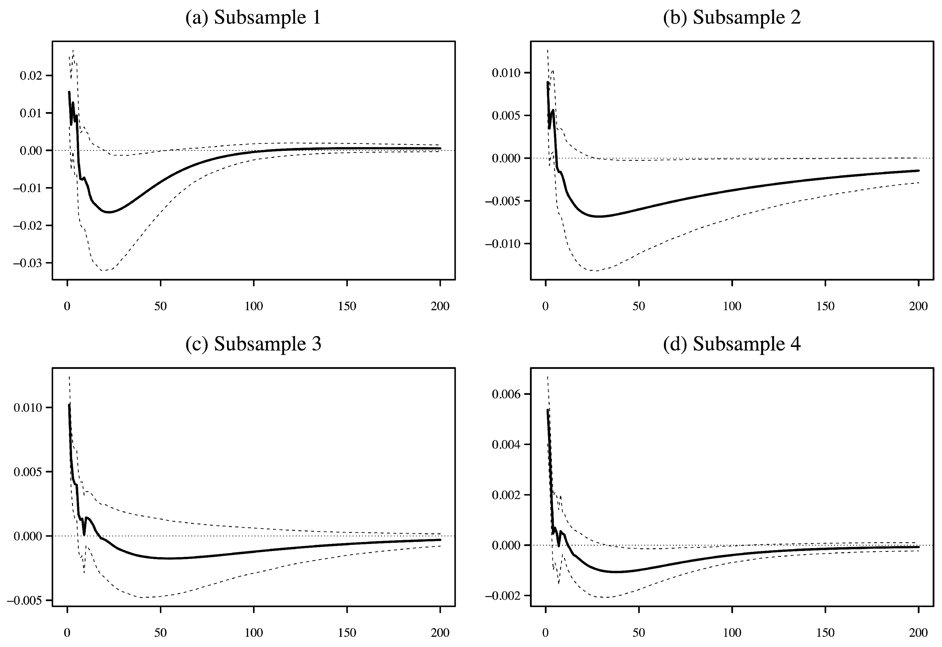
Plots of the GIRFs derived from the VAR model are presented in Figure 4, Figure 5, Figure 6, Figure 7, Figure 8 and Figure 9, organized as single impulse response pairs shown for each of subsamples 1–4 in panels (a–d), respectively. The GIRFs are shown for 200 steps ahead with 90-percent confidence intervals bootstrapped using 200 iterations. Note that 50 steps ahead represents just over 4 hours of trading time.
Figure 4 and Figure 5 indicate that a one standard deviation shock in PROF is associated with an immediate and generally short-lived negative response in the relative bid–ask spreads of both New York and Tokyo. This suggests that, in the short term, liquidity improves in both markets following an arbitrage profit opportunity, as arbitragers act as “cross-sectional market makers” as described by Holden (1995). Accordingly, we conclude that the deviations from the LOOP that lead to arbitrage opportunities in platinum futures are generally due to non-fundamental demand shocks.
Furthermore, the immediate liquidity-enhancing effect of an arbitrage profit shock is greater when the futures contract is less actively traded. The size of the immediate liquidity response is greatest for SPNY in subsample 1, as shown in Figure 4a, which is when the New York contract is least actively traded. The opposite is true for SPTO in that the liquidity response is greatest in subsample 4, as shown in Figure 5d, at the time when the Tokyo contract is least actively traded. The peak of the immediate liquidity response in New York decreases monotonically over subsamples 1–4, while it increases in Tokyo. The liquidity-enhancing effect of arbitrage profit opportunities is not only greater but also more persistent when a market is less actively traded, consistent with the findings of Rappoport and Tuzun (2020) for equity and bond markets.
An interesting feature of the GIRFs when the contract in each market is most actively traded, which is in subsample 4 for New York shown in Figure 4d and in subsample 1 for Tokyo shown in Figure 5a, is the small but persistent positive marginal spreads that began within 50 steps following the PROF shock. This may seem inconsistent with our non-fundamental demand shock explanation. Does this delayed decrease in liquidity suggest the arbitrage opportunity is first mistaken for a non-fundamental demand shock and shortly after recognized to be the result of asymmetric information? Given that we observe this effect only when the respective contract is most actively traded, we favor an alternative and more plausible interpretation. In response to a demand shock, the resulting highly liquid market can lead to a deterioration in liquidity, as predicted by Admati and Pfleiderer (1988). Discretionary liquidity traders prefer to trade when they have little impact on prices to minimize their losses to informed traders. Greater liquidity trading encourages more informed trading at the same time, but competition between informed traders reduces their total profit. This benefits liquidity traders and encourages their further participation. Liquidity will eventually deteriorate when the concentration of informed traders increases the cost of adverse selection. Thus, for highly liquid markets, arbitrage associated with a non-fundamental demand shock may lead to an immediate increase in liquidity, followed by a persistent decrease in liquidity relative to before the shock.
Figure 6 and Figure 7 show the response of PROF to a one standard deviation positive shock in SPNY and SPTO, respectively. The immediate response is negative in all cases, which seems inconsistent with the notion that a decrease in liquidity should increase arbitrage profit opportunities. However, the immediate negative response is explained by how the widening of the relative spread affects the calculation of arbitrage profit. A positive shock in the relative spread represents a decrease in or negative shock to liquidity and occurs via an increase in the ask price, a decrease in the bid price or both. The change in ask or bid prices due to the shock decreases PROF on impact, as Equation (1) suggests. As time passes, the deviation from the LOOP increases as traders find more room for arbitrage following the negative liquidity shock. The positive response of PROF is most apparent for liquidity shocks originating in subsample 4 for New York (Figure 6d) and in subsample 1 for Tokyo (Figure 7a). Thus, the positive effect on arbitrage opportunity is larger when the negative liquidity shock comes from a market in the actively traded phase of its lifespan. The positive response is less apparent in Figure 6a–c for subsamples 1, 2 and 3, respectively, and Figure 7b–d for subsamples 2, 3 and 4, respectively. This is because the liquidity shock in these subsamples originates from a market with relatively few active traders and is less likely to lead to a meaningful increase in opportunities for arbitrage between New York and Tokyo. The magnitudes of the PROF responses to liquidity shocks from each spread are comparable, except in Figure 6a for subsample 1, when the New York market is relatively inactive.
Figure 8 and Figure 9 show the response of SPTO to a shock in SPNY and the response of SPNY to a shock in SPTO, respectively. A positive shock in the relative spread of one market initially results in an increase in the relative spread of the other market. This reflects liquidity commonality, defined as the co-movement in liquidity across securities or markets that are driven by one or more common factors. Chordia et al. (2000) identified liquidity commonality in U.S. stocks, while Marshall et al. (2013b) and Caporin et al. (2015) provided evidence for a systematic liquidity factor in commodity futures markets. However, as time goes on, the positive response weakens, and spreads generally narrow as traders find that the source of the spread increase is non-fundamental. The latter liquidity-enhancing effect dominates in all subsamples, except for subsample 1 in Figure 8a. The liquidity-enhancing effect is of greater magnitude when the impulse market is in a more active part of its lifespan and the response market is less active. This can be observed clearly in Figure 8d for subsample 4 and Figure 9a for subsample 1.
5. Conclusions
Arbitrage and liquidity in markets for substitute securities are closely related. Theory posits reasons by which arbitrage should affect liquidity and liquidity should affect arbitrage. Whether arbitrage opportunities are associated with enhanced or diminished liquidity depends on the reason behind why the arbitrage opportunity has arisen. Non-fundamental demand shocks enhance liquidity, while asymmetric information diminishes or is toxic to liquidity.
Arbitrage profit opportunities in futures markets trading an identical underlying grade of platinum in New York and Tokyo generally lead to increased liquidity in both markets. This suggests that non-fundamental demand shocks are the predominant cause of deviations from the LOOP across the two markets. The liquidity improvement is larger during periods of a contract’s lifespan in which it is less actively traded. When a contract is most actively traded, liquidity first improves in response to an arbitrage opportunity and then deteriorates. This is consistent with the notion proposed by Admati and Pfleiderer (1988) that discretionary liquidity and informed traders may concentrate their transactions following non-fundamental demand shocks, and subsequently, liquidity declines as the risk of adverse selection rises. In particular, when the contracts are in an actively traded phase of their lifespan, a negative liquidity shock is associated with greater room for arbitrage between the two major future markets for platinum. A degree of relative liquidity commonality was observed across the two markets over the entirety of the contracts’ lifespans.
Our results suggest that non-fundamental demand shocks, which are the main source of arbitrage opportunities between the New York and Tokyo markets, provide opportunities for both hedgers and speculators to trade, facilitated by liquidity provision from market participants performing the role of discretionary liquidity traders. Demand shocks provide a relatively advantageous opportunity for market participants to transact even when the contract in question is not in an actively traded phase of its lifespan.
Understanding the causal relationship between arbitrage and liquidity is important for commodity futures markets, given that multiple exchanges list contracts based on identical underlying commodities which are traded concurrently in overlapping day and night trading sessions. There is a number of potential directions for extending the research on this relationship in commodity futures markets. Although our research suggests toxic arbitrage is not prevalent in platinum futures, a switching regime approach may be used to better understand the circumstances around which arbitrage leads to lower market liquidity. Panel VAR models may be used to examine a series of contracts over time for a single underlying commodity or for multiple related commodity futures contracts at a point in time.
Author Contributions
Conceptualization, K.I. and C.W.; methodology, K.I. and C.W.; software, C.W.; validation, K.I. and C.W.; formal analysis, C.W.; investigation, K.I. and C.W.; resources, K.I. and C.W.; data curation, K.I.; writing—original draft preparation, C.W.; writing—review and editing, K.I. and C.W.; visualization, C.W.; supervision, K.I.; project administration, K.I.; funding acquisition, K.I. All authors have read and agreed to the published version of the manuscript.
Funding
This work is supported by JSPS KAKENHI Grant Numbers 19K01754 and 22K18529.
Data Availability Statement
Data were obtained from Thomson Reuters (now Refinitiv), Bloomberg and the Tokyo Commodity Exchange.
Acknowledgments
We thank Michael McAleer for his helpful comments and Tao Xu for assistance in compiling the data.
Conflicts of Interest
The authors declare no conflict of interest.
| 1 | NYMEX is part of the CME Group, and TOCOM is part of the Japan Exchange Group. |
| 2 | The NYMEX platinum contract specifications can be found at https://www.cmegroup.com/markets/metals/precious/platinum.contractSpecs.html (accessed on 3 May 2019). The TOCOM platinum standard contract specifications can be found at https://www.jpx.co.jp/english/derivatives/products/precious-metals/platinum-standard-futures/01.html (accessed on 3 May 2019). |
| 3 | Note that in addition to limits in the expiry month, TOCOM imposes looser position limits in the month before the expiry month and the second contract month. There is also a position limit for all contract months combined. |
| 4 | TOCOM extended its trading hours after the sample period of our study. The day session now opens at 8:45 a.m. JST and closes at 3:15 p.m. The night session runs from 4:30 p.m. to 6:00 a.m. the next day. |
| 5 | Forward exchange rates are used for the currency conversion presuming that the arbitrage trades between the New York and Tokyo markets are held to expiry. 12-month LIBOR rates are used when the futures have between 12 and 6 months to expiry, 6-month rates for when the contracts have between 6 and 3 months to expiry, the 2-month rates for when the contracts have between 2 months and 1 month to expiry, 1-month rates for when the contracts have between 1 month and 1 week to expiry, and 1-week rates are used for the contracts when they have less than 1 week to expiry. One gram is equivalent to 0.03215 troy ounces. |
References
- Admati, Anat R., and Paul Pfleiderer. 1988. Theory of Intraday Patterns: Volume and Price Variability A Theory of Intraday Patterns: Volume and Price Variability. The Review of Financial Studies 1: 3–40. [Google Scholar] [CrossRef] [Green Version]
- Bohl, Martin T., Alexander Pütz, and Christoph Sulewski. 2021. Speculation and the informational efficiency of commodity futures markets. Journal of Commodity Markets 23: 100159. [Google Scholar] [CrossRef]
- Boos, Dominik, and Linus Grob. 2022. Tracking speculative trading. Journal of Financial Markets, 100774. [Google Scholar] [CrossRef]
- Boubaker, Sabri, Zhenya Liu, Shanglin Lu, and Yifan Zhang. 2021. Trading signal, functional data analysis and time series momentum. Finance Research Letters 42: 101933. [Google Scholar] [CrossRef]
- Caporin, Massimiliano, Angelo Ranaldo, and Gabriel G Velo. 2015. Precious metals under the microscope: A high-frequency analysis. Quantitative Finance 15: 743–59. [Google Scholar] [CrossRef] [Green Version]
- Chordia, Tarun, Richard Roll, and Avanidhar Subrahmanyam. 2000. Commonality in liquidity. Journal of Financial Economics 56: 3–28. [Google Scholar] [CrossRef]
- Foucault, Thierry, Roman Kozhan, and Wing Wah Tham. 2017. Toxic arbitrage. Review of Financial Studies 30: 1053–94. [Google Scholar] [CrossRef]
- Ghadhab, Imen. 2018. Arbitrage opportunities and liquidity: An intraday event study on cross-listed stocks. Journal of Multinational Financial Management 46: 1–10. [Google Scholar] [CrossRef]
- Gromb, Denis, and Dimitri Vayanos. 2010. Limits of Arbitrage: The State of the Theory. National Bureau of Economic Research, Working Paper 15821. Cambridge: National Bureau of Economic Research. [Google Scholar] [CrossRef]
- Holden, Craig W. 1995. Index arbitrage as cross-sectional market making. Journal of Futures Markets 15: 423–55. [Google Scholar] [CrossRef]
- Iwatsubo, Kentaro, and Clinton Watkins. 2020. Who influences the fundamental value of commodity futures in Japan? International Review of Financial Analysis 67: 1–15. [Google Scholar] [CrossRef]
- Iwatsubo, Kentaro, Clinton Watkins, and Tao Xu. 2018. Intraday seasonality in efficiency, liquidity, volatility and volume: Platinum and gold futures in Tokyo and New York. Journal of Commodity Markets 11: 59–71. [Google Scholar] [CrossRef] [Green Version]
- Johannsen, Kolja. 2017. Toxic Arbitrage and Price Discovery. Available online: https://ssrn.com/abstract=2950161 (accessed on 6 March 2019). [CrossRef]
- Johnson Matthey. 2016. PGM Market Report May 2016. Johnson Matthey Technology Review, 60. London: Johnson Matthey. [Google Scholar] [CrossRef]
- Kumar, Praveen, and Duane J. Seppi. 1994. Information and Index Arbitrage. The Journal of Business 67: 481–509. [Google Scholar] [CrossRef]
- Kwon, Kyung Yoon, Jangkoo Kang, and Jaesun Yun. 2020. Weekly momentum in the commodity futures market. Finance Research Letters 35: 1–8. [Google Scholar] [CrossRef]
- Kyle, Albert S. 1985. Continuous Auctions and Insider Trading. Econometrica 53: 1315–35. [Google Scholar] [CrossRef] [Green Version]
- Lauter, Tobias, and Marcel Prokopczuk. 2022. Measuring commodity market quality. Journal of Banking and Finance 145: 106658. [Google Scholar] [CrossRef]
- Ludwig, Michael. 2019. Speculation and its impact on liquidity in commodity markets. Resources Policy 61: 532–47. [Google Scholar] [CrossRef]
- Marshall, Ben R., Nhut H. Nguyen, and Nuttawat Visaltanachoti. 2013a. ETF arbitrage: Intraday evidence. Journal of Banking and Finance 37: 3486–98. [Google Scholar] [CrossRef]
- Marshall, Ben R., Nhut H. Nguyen, and Nuttawat Visaltanachoti. 2013b. Liquidity commonality in commodities. Journal of Banking and Finance 37: 11–20. [Google Scholar] [CrossRef]
- McDonald, Donald, and Leslie B. Hunt. 1982. A History of Platinum and Its Allied Metals. London: Johnson Matthey. [Google Scholar]
- Pesaran, H. Hashem, and Yongcheol Shin. 1998. Generalized impulse response analysis in linear multivariate models. Economics Letters 58: 17–29. [Google Scholar] [CrossRef]
- Rappoport, David Elias, and Tugkan Tuzun. 2020. Arbitrage and Liquidity: Evidence from a Panel of Exchange Traded Funds. Finance and Economics Discussion Series 2020-097; Washington, DC: Board of Governors of the Federal Reserve System. [Google Scholar] [CrossRef]
- Roll, Richard, Eduardo Schwartz, and Avanidhar Subrahmanyam. 2007. Liquidity and the Law of One Price: The Case of the Futures-Cash Basis. Journal of Finance 62: 2201–34. [Google Scholar] [CrossRef] [Green Version]
- Rösch, Dominik. 2021. The impact of arbitrage on market liquidity. Journal of Financial Economics 142: 195–213. [Google Scholar] [CrossRef]
- Sakkas, Athanasios, and Nikolaos Tessaromatis. 2020. Factor based commodity investing. Journal of Banking and Finance 115: 105807. [Google Scholar] [CrossRef]
- Schultz, Paul, and Sophie Shive. 2010. Mispricing of dual-class shares: Profit opportunities, arbitrage, and trading. Journal of Financial Economics 98: 524–49. [Google Scholar] [CrossRef]
- Shleifer, Andrei, and Robert W. Vishny. 1997. The limits of arbitrage. Journal of Finance 52: 35–55. [Google Scholar] [CrossRef]
- Sun, Hang, Jaap W. B. Bos, and Paulo Rodrigues. 2023. Destabilizing or passive? The impact of commodity index traders on equilibrium prices. International Review of Economics and Finance 83: 271–85. [Google Scholar] [CrossRef]
- Vigne, Samuel A., Brian M. Lucey, Fergal A. O’Connor, and Larisa Yarovaya. 2017. The financial economics of white precious metals—A survey. International Review of Financial Analysis 52: 292–308. [Google Scholar] [CrossRef]
- Wilson, Paul. 2015. WPIC Platinum Quarterly Q2 2015. London: World Platinum Investment Council. [Google Scholar]
Figure 1.
Daily prices for the April 2016 futures on TOCOM and NYMEX. (Note: The figure shows the daily April 2016 futures prices for platinum on NYMEX and TOCOM in US dollars per troy ounce on the RHS axis and Japanese yen per kilogram on the LHS axis).
Figure 1.
Daily prices for the April 2016 futures on TOCOM and NYMEX. (Note: The figure shows the daily April 2016 futures prices for platinum on NYMEX and TOCOM in US dollars per troy ounce on the RHS axis and Japanese yen per kilogram on the LHS axis).
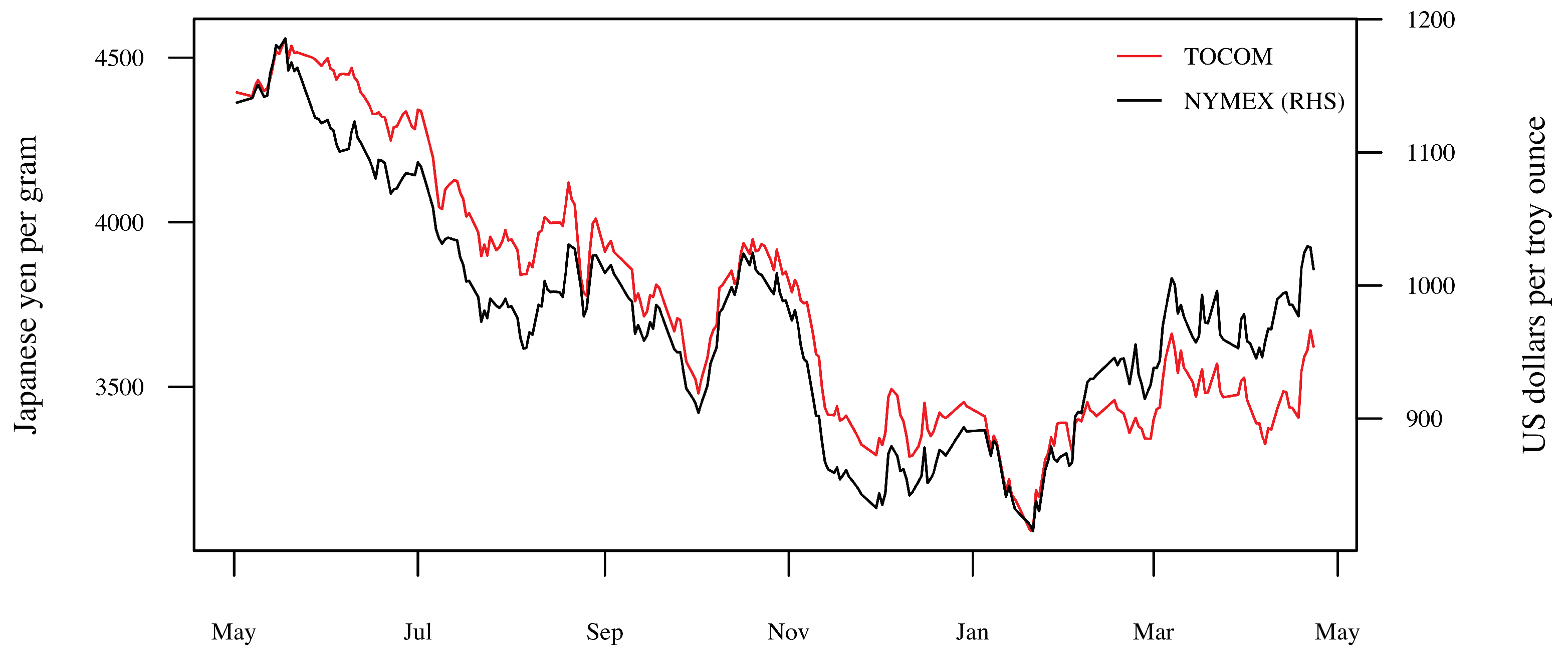
Figure 2.
Arbitrage profit and liquidity variables. (Note: The figure shows the 5 min of average arbitrage profit (PROF) and the relative bid–ask spreads for the NYMEX (SPNY) and TOCOM (SPTO) contracts calculated from 1 min data for 264 trading days starting at 9:00 a.m. Japan Standard Time (JST) on 7 May 2015 and ending at 4:00 a.m. JST on 23 April 2016 in basis points in panels (a–c), respectively. The shaded regions indicate the five subsamples).
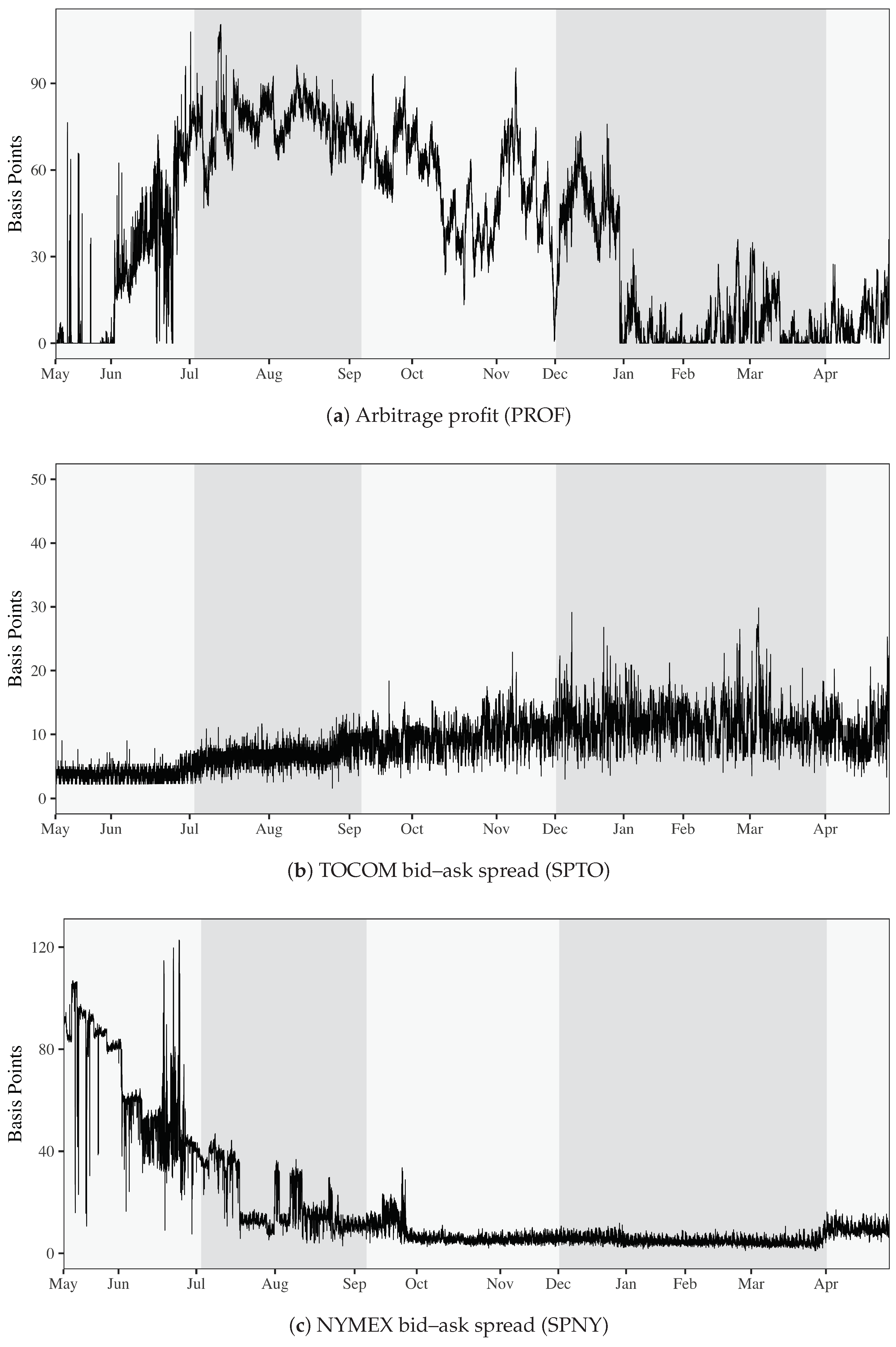
Figure 3.
Platinum futures contract volumes on TOCOM and NYMEX (Notes: Panels (a,b) show the 5-min aggregate trading volumes for the TOCOM (VOLTO) and NYMEX (VOLNY) April 2016 platinum futures contracts over 264 trading days starting at 9:00 a.m. Japan Standard Time (JST) on 7 May 2015 and ending at 4:00 a.m. JST on 23 April 2016, respectively. Panel (c) provides the cumulative total trading volume for the April 2016 contract on each exchange over the sample period. The shaded regions indicate the five subsamples).
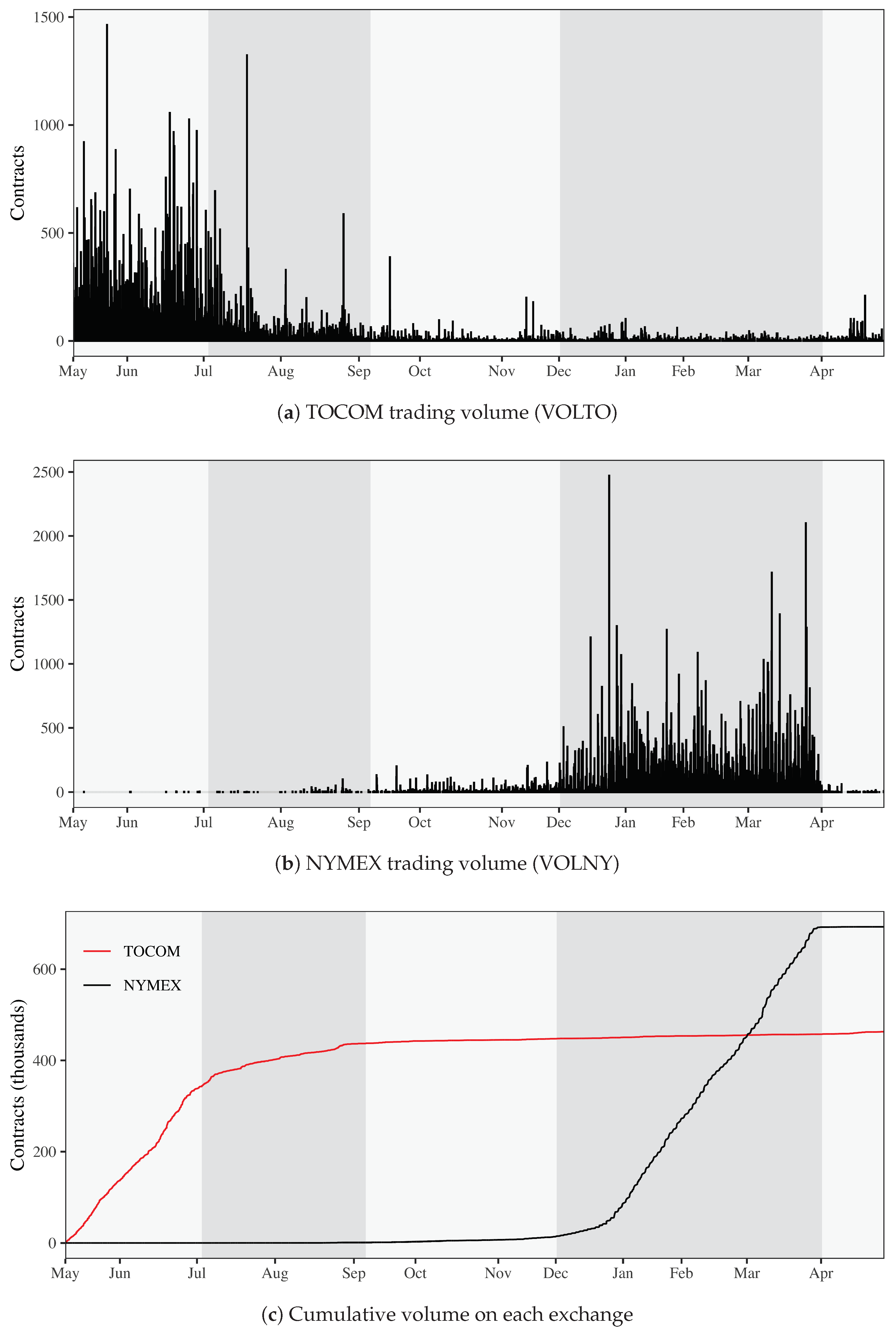
Figure 4.
Response of SPNY to a shock in PROF. (Notes: The solid lines represent the 200-step-ahead GIRFs. The dashed lines show 90-percent confidence intervals bootstrapped using 200 iterations).
Figure 4.
Response of SPNY to a shock in PROF. (Notes: The solid lines represent the 200-step-ahead GIRFs. The dashed lines show 90-percent confidence intervals bootstrapped using 200 iterations).

Figure 5.
Response of SPTO to a shock in PROF. (Notes: The solid lines represent the 200-step-ahead GIRFs. The dashed lines show 90-percent confidence intervals bootstrapped using 200 iterations).
Figure 5.
Response of SPTO to a shock in PROF. (Notes: The solid lines represent the 200-step-ahead GIRFs. The dashed lines show 90-percent confidence intervals bootstrapped using 200 iterations).
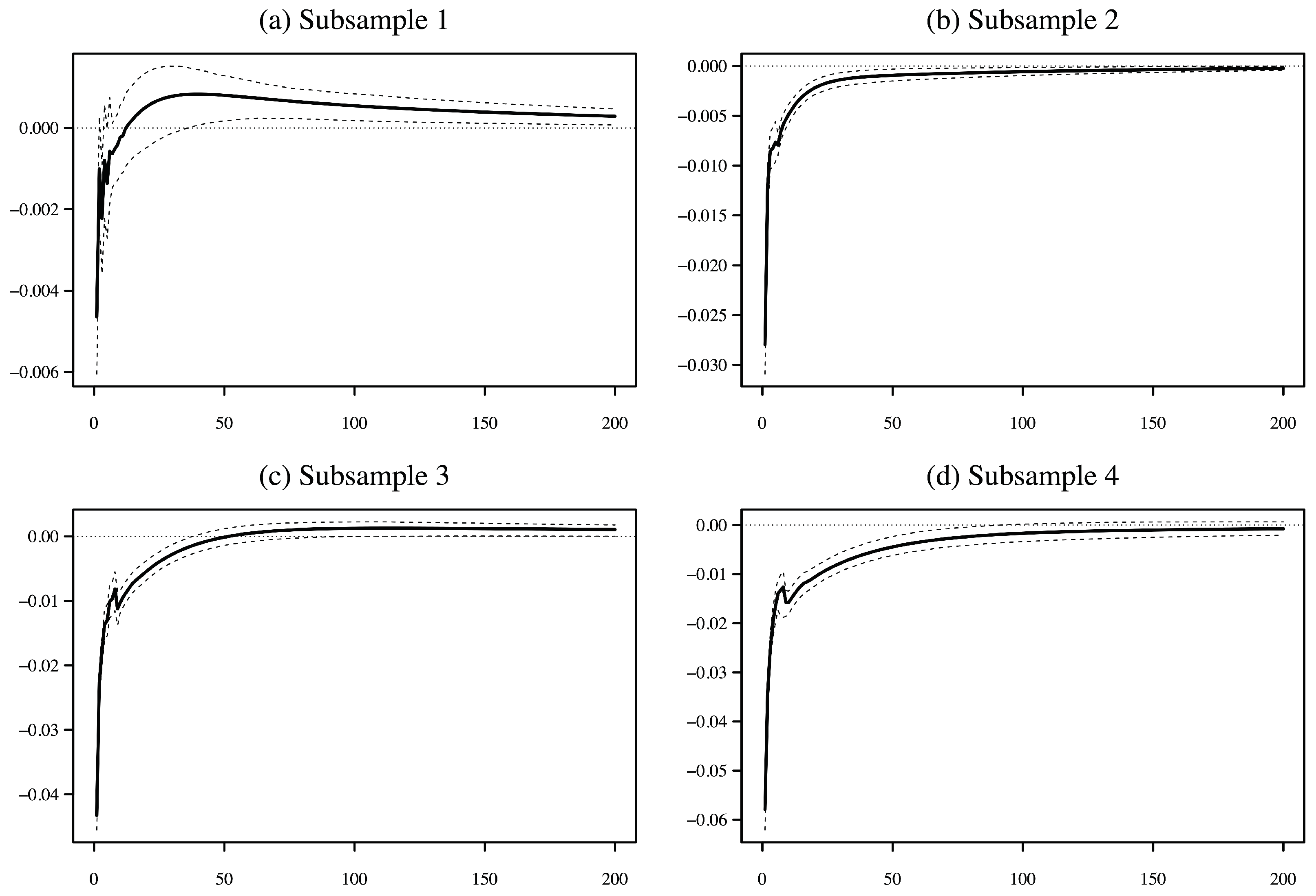
Figure 6.
Response of PROF to a shock in SPNY. (Notes: The solid lines represent the 200-step-ahead GIRFs. The dashed lines show 90-percent confidence intervals bootstrapped using 200 iterations).
Figure 6.
Response of PROF to a shock in SPNY. (Notes: The solid lines represent the 200-step-ahead GIRFs. The dashed lines show 90-percent confidence intervals bootstrapped using 200 iterations).
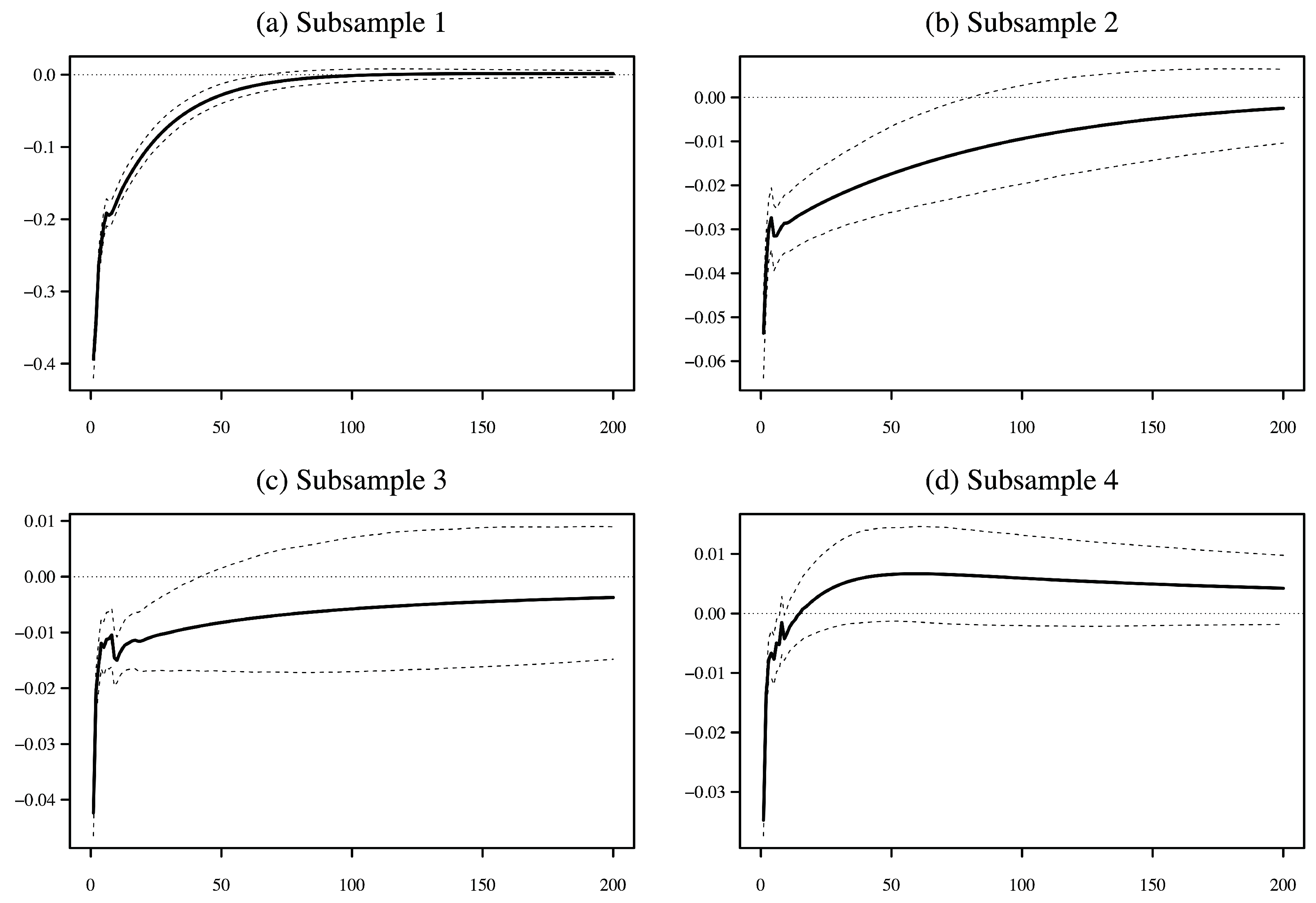
Figure 7.
Response of PROF to a shock in SPTO. (Notes: The solid lines represent the 200-step-ahead GIRFs. The dashed lines show 90-percent confidence intervals bootstrapped using 200 iterations).
Figure 7.
Response of PROF to a shock in SPTO. (Notes: The solid lines represent the 200-step-ahead GIRFs. The dashed lines show 90-percent confidence intervals bootstrapped using 200 iterations).
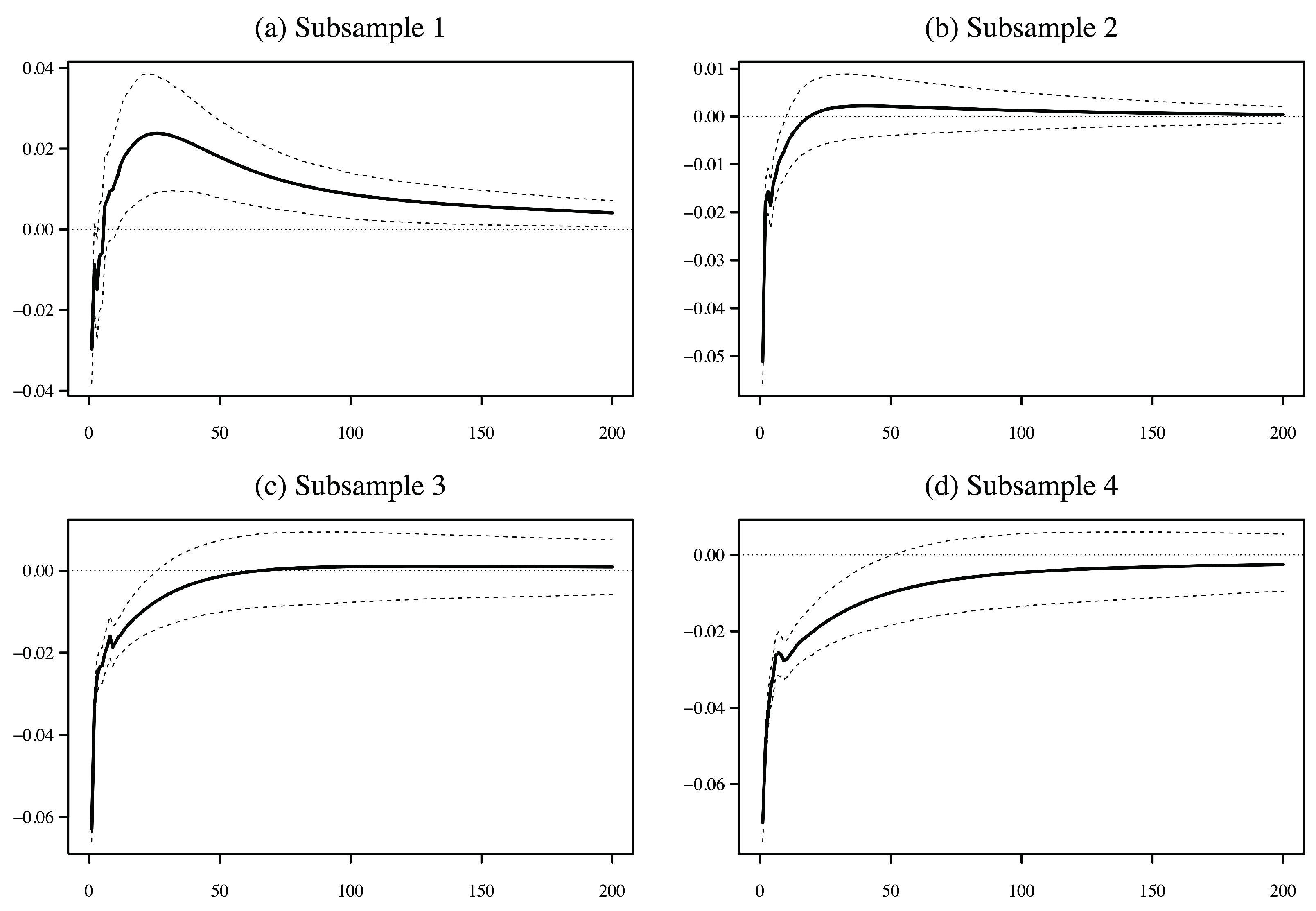
Figure 8.
Response of SPTO to a shock in SPNY. (Notes: The solid lines represent the 200-step-ahead GIRFs. The dashed lines show 90-percent confidence intervals bootstrapped using 200 iterations).
Figure 8.
Response of SPTO to a shock in SPNY. (Notes: The solid lines represent the 200-step-ahead GIRFs. The dashed lines show 90-percent confidence intervals bootstrapped using 200 iterations).
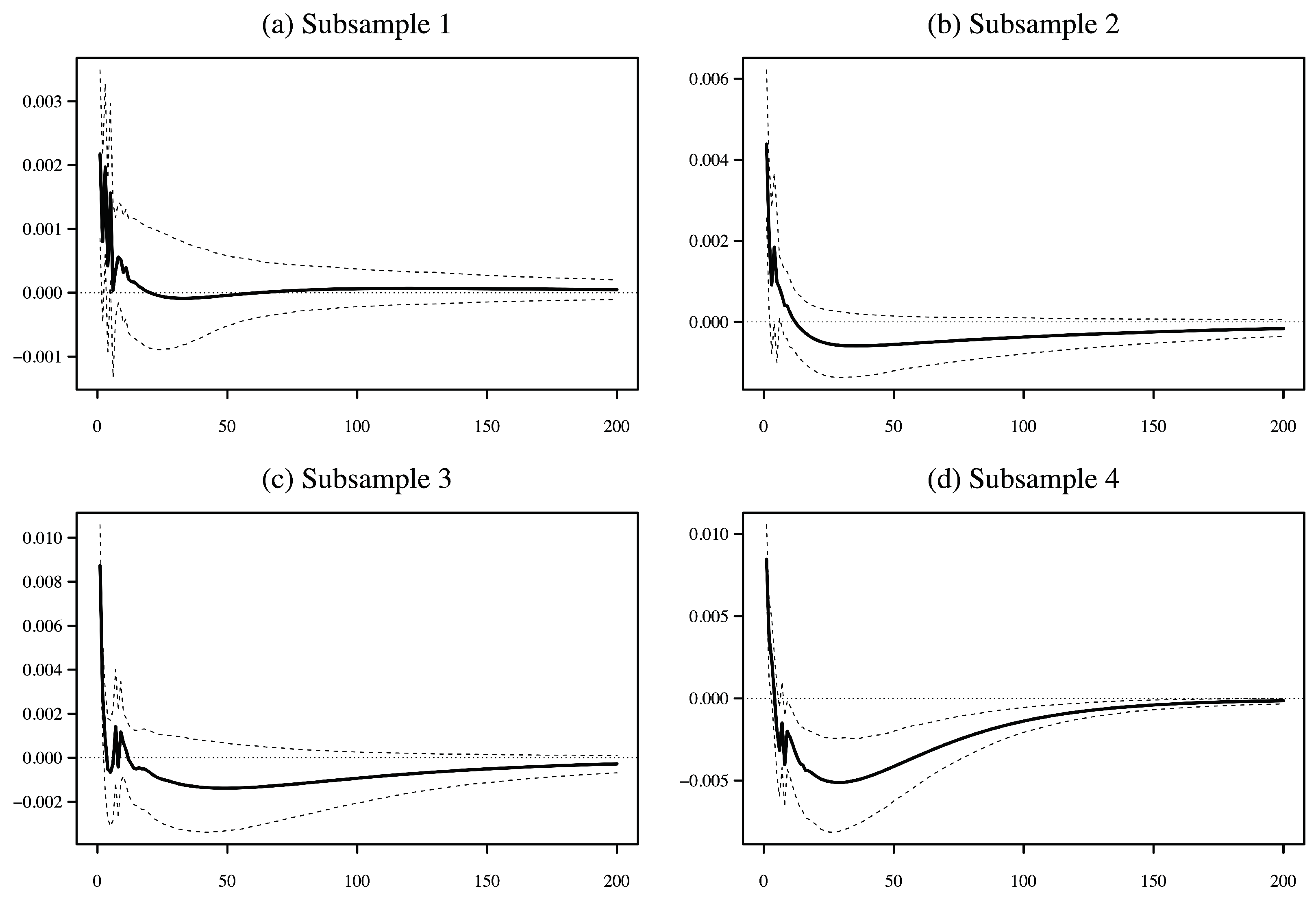
Figure 9.
Response of SPNY to a shock in SPTO. (Notes: The solid lines represent the 200-step-ahead GIRFs. The dashed lines show 90-percent confidence intervals bootstrapped using 200 iterations).
Figure 9.
Response of SPNY to a shock in SPTO. (Notes: The solid lines represent the 200-step-ahead GIRFs. The dashed lines show 90-percent confidence intervals bootstrapped using 200 iterations).

Table 1.
The April 2016 futures contracts on NYMEX and TOCOM and the subsamples.
| 2015 | 2016 | |||||||||||
|---|---|---|---|---|---|---|---|---|---|---|---|---|
| Exchange | May | Jun. | Jul. | Aug. | Sep. | Oct. | Nov. | Dec. | Jan. | Feb. | Mar. | Apr. |
| TOCOM | Farthest | 2nd Farthest | 3rd Farthest | 3rd Nearest | 2nd Nearest | Nearest | ||||||
| NYMEX | 11 | 10 | 9 | 8 | 7 | 6 | 5 | 4 | 3 | 2 | 1 | Expiry |
| Subsamples | 1 | 2 | 3 | 4 | 5 | |||||||
Notes: The TOCOM contract is denoted using the nearest and farthest nomenclature. The NYMEX contract is labeled in terms of months before the expiration month. The shaded regions indicate the five subsamples.
Table 2.
Summary statistics for the arbitrage and liquidity variables.
| Full Sample | Subsample 1 | Subsample 2 | |||||||
| PROF | SPTO | SPNY | PROF | SPTO | SPNY | PROF | SPTO | SPNY | |
| Mean | 0.0040 | 0.0009 | 0.0020 | 0.0024 | 0.0004 | 0.0066 | 0.0077 | 0.0007 | 0.0020 |
| Median | 0.0043 | 0.0009 | 0.0007 | 0.0021 | 0.0004 | 0.0061 | 0.0077 | 0.0007 | 0.0014 |
| Minimum | 0.0000 | 0.0002 | 0.0001 | 0.0000 | 0.0002 | 0.0008 | 0.0047 | 0.0002 | 0.0003 |
| Maximum | 0.0110 | 0.0030 | 0.0127 | 0.0108 | 0.0009 | 0.0127 | 0.0110 | 0.0013 | 0.0047 |
| St. Dev. | 0.0031 | 0.0004 | 0.0025 | 0.0025 | 0.0001 | 0.0021 | 0.0009 | 0.0001 | 0.0011 |
| Skewness | −0.03 | 0.56 | 1.83 | 0.66 | 0.38 | 0.12 | 0.18 | 0.53 | 0.75 |
| Ex. Kurtosis | −1.46 | 0.81 | 2.32 | −0.73 | 0.84 | −1.19 | 1.75 | 1.51 | −1.00 |
| Unit Root | −5.66 | −61.13 | −10.09 | −12.76 | −54.53 | −16.92 | −7.23 | −58.49 | −8.05 |
| P-value | 0.01 | 0.01 | 0.01 | 0.01 | 0.01 | 0.01 | 0.01 | 0.01 | 0.01 |
| Observations | 41,322 | 41,322 | 41,322 | 7455 | 7455 | 7455 | 8946 | 8946 | 8946 |
| Subsample 3 | Subsample 4 | Subsample 5 | |||||||
| PROF | SPTO | SPNY | PROF | SPTO | SPNY | PROF | SPTO | SPNY | |
| Mean | 0.0055 | 0.0010 | 0.0007 | 0.0015 | 0.0012 | 0.0005 | 0.0007 | 0.0011 | 0.0010 |
| Median | 0.0057 | 0.0010 | 0.0006 | 0.0005 | 0.0012 | 0.0005 | 0.0006 | 0.0010 | 0.0010 |
| Minimum | 0.0001 | 0.0003 | 0.0002 | 0.0000 | 0.0003 | 0.0001 | 0.0000 | 0.0003 | 0.0004 |
| Maximum | 0.0095 | 0.0023 | 0.0034 | 0.0076 | 0.0030 | 0.0013 | 0.0036 | 0.0025 | 0.0017 |
| St. Dev. | 0.0016 | 0.0002 | 0.0004 | 0.0019 | 0.0003 | 0.0001 | 0.0006 | 0.0003 | 0.0002 |
| Skewness | −0.33 | 0.49 | 2.01 | 1.17 | 1.22 | 0.83 | 0.68 | 1.31 | 0.55 |
| Ex. Kurtosis | −0.29 | 0.63 | 4.02 | −0.09 | 3.51 | 1.04 | −0.28 | 2.64 | 0.37 |
| Unit Root | -3.91 | −34.24 | −22.98 | −5.12 | −30.88 | -60.67 | −7.24 | −13.37 | −24.26 |
| P-value | 0.01 | 0.01 | 0.01 | 0.01 | 0.01 | 0.01 | 0.01 | 0.01 | 0.01 |
| Observations | 10,437 | 10,437 | 10,437 | 14,484 | 14,484 | 14,484 | 3408 | 3408 | 3408 |
Notes: PROF represents arbitrage profit. SPNY and SPTO are the relative bid–ask spreads for the April 2016 platinum futures contracts traded on NYMEX and TOCOM, respectively. Each variable is constructed using 1 min data, and the result is averaged over 5 min periods. The table shows summary statistics for the full sample and each subsample calculated from the 5 min data. Unit Root and P-value represent the Phillips–Perron test statistic and its associated p-value for a 5% level of significance.
Table 3.
Summary statistics for trading volume during each 5 min interval for each sample.
| Full Sample | Subsample 1 | Subsample 2 | ||||
| VOLTO | VOLNY | VOLTO | VOLNY | VOLTO | VOLNY | |
| Mean | 11.08 | 16.75 | 46.02 | 0.00 | 10.51 | 0.10 |
| St. Dev. | 39.65 | 58.04 | 77.36 | 0.10 | 29.96 | 1.59 |
| Skewness | 10.90 | 10.32 | 5.57 | 31.34 | 15.89 | 36.71 |
| Ex. Kurtosis | 202.98 | 215.55 | 50.81 | 1150.56 | 501.97 | 1885.75 |
| Maximum | 1464 | 2471 | 1464 | 5 | 1323 | 99 |
| Sum | 457,723 | 692,167 | 343,072 | 30 | 94,006 | 904 |
| Subsample 3 | Subsample 4 | Subsample 5 | ||||
| VOLTO | VOLNY | VOLTO | VOLNY | VOLTO | VOLNY | |
| Mean | 1.03 | 1.33 | 0.69 | 46.77 | 1.56 | 0.19 |
| St. Dev. | 6.48 | 7.83 | 3.47 | 90.43 | 6.98 | 2.07 |
| Skewness | 29.02 | 15.88 | 11.36 | 6.76 | 13.71 | 21.45 |
| Ex. Kurtosis | 1403.95 | 340.72 | 189.45 | 93.15 | 292.49 | 526.09 |
| Maximum | 388 | 230 | 102 | 2471 | 209 | 62 |
| Sum | 10,713 | 13,833 | 9932 | 677,400 | 5321 | 632 |
Notes: VOLTO and VOLNY represent the aggregate 5 min trading volumes in the April 2016 platinum futures contracts traded on TOCOM and NYMEX, respectively. Maximum indicates the largest number of contracts traded within the 5 min time intervals. The minimum for all subsamples is zero contracts for both exchanges and is not shown in the table. Sum provides the total number of contracts traded during each subsample for each exchange.
Table 4.
Granger causality F-statistics.
| Null Hypothesis | Subsample 1 | Subsample 2 | Subsample 3 | Subsample 4 |
|---|---|---|---|---|
| PROF does not Granger cause SPNY or SPTO | 5.40 *** | 2.12 *** | 2.32 *** | 3.70 *** |
| SPTO does not Granger cause SPNY or PROF | 5.55 *** | 16.89 *** | 6.73 *** | 6.21 *** |
| SPNY does not Granger cause SPTO or PROF | 6.48 *** | 1.63 *** | 4.14 *** | 11.63 *** |
Notes: PROF represents arbitrage profit. SPNY and SPTO are the relative bid–ask spreads for the April 2016 platinum futures contracts traded on NYMEX and TOCOM, respectively. The table shows the Granger causality F-statistic. ***, ** and * indicate significance at the 1%, 5% and 10% levels, respectively.
Publisher’s Note: MDPI stays neutral with regard to jurisdictional claims in published maps and institutional affiliations. |
© 2022 by the authors. Licensee MDPI, Basel, Switzerland. This article is an open access article distributed under the terms and conditions of the Creative Commons Attribution (CC BY) license (https://creativecommons.org/licenses/by/4.0/).
Share and Cite
MDPI and ACS Style
Iwatsubo, K.; Watkins, C. Causality between Arbitrage and Liquidity in Platinum Futures. J. Risk Financial Manag. 2022, 15, 593. https://doi.org/10.3390/jrfm15120593
AMA Style
Iwatsubo K, Watkins C. Causality between Arbitrage and Liquidity in Platinum Futures. Journal of Risk and Financial Management. 2022; 15(12):593. https://doi.org/10.3390/jrfm15120593
Chicago/Turabian StyleIwatsubo, Kentaro, and Clinton Watkins. 2022. "Causality between Arbitrage and Liquidity in Platinum Futures" Journal of Risk and Financial Management 15, no. 12: 593. https://doi.org/10.3390/jrfm15120593