
Volatility Spillover among Japanese Sectors in Response to COVID-19

1
Graduate School of Science and Technology, Kwansei Gakuin University, 2-1 Gakuen, Sanda 669-1337, Hyogo, Japan
2
School of Science, Kwansei Gakuin University, 2-1 Gakuen, Sanda 669-1337, Hyogo, Japan
*
Author to whom correspondence should be addressed.
J. Risk Financial Manag. 2022, 15(10), 480; https://doi.org/10.3390/jrfm15100480
Submission received: 21 September 2022
/
Revised: 17 October 2022
/
Accepted: 17 October 2022
/
Published: 20 October 2022
(This article belongs to the Special Issue Public Economics and Finance Pre-during-Post COVID-19 Pandemic)
Abstract
:This study clarifies how risks spread across economic sectors and indicates the sectors that are the most affected to help investors with asset allocation and to support them in risk management. Although the Japanese stock market is one of the relatively large global stock markets, no studies have explored volatility spillovers among its sectors. Using the forecast error variance decomposition of the vector autoregressive model, this study examines the volatility spillovers among sectors classified on the Tokyo Stock Exchange. Our findings show that the pattern of volatility spillovers across sectors in the Japanese stock market differs between a few years preceding the coronavirus disease 2019 (pre-COVID-19), from 2014 to 2019, and during the COVID-19 period, in 2020. Although the energy resources and bank sectors are risk receivers in the pre-COVID-19 period, these sectors are risk transmitters during the COVID-19 period. We also find that volatility spillovers in the Japanese stock market are mainly driven by negative realized semivariance. These results are useful for asset allocation and risk management.
1. Introduction
Interdependence between financial markets has increased with financial liberalization, which increases the vulnerability of markets to domestic and international events and shocks and reduces the diversification effect. For example, a huge shocks that occurs in one market can spread to other markets rapidly, like the global financial crisis in 2007 and 2008, the Chinese shock in 2015, and COVID-19 in 2020. In this context, volatility spillovers have attracted much attention recently. Volatility spillovers play an important role for investors by enhancing their asset allocation, investment strategies, and risk management. However, the direction and magnitude of volatility spillovers vary depending on market conditions and asset types. Therefore, studies of volatility spillover have been conducted not only among international stock markets (Li 2021) and domestic sectors (Mensi et al. 2021), but also among various financial instruments, such as among banks (Diebold and Yilmaz 2014), between oil price and stock sectors (Kang et al. 2021), between VIX and stock sectors (Ahmad et al. 2021), economic policy uncertainty and oil price (Yang 2019), foreign exchange and stock markets (Grobys 2015), and among cryptocurrencies (Kumar and Anandarao 2019) using some quantified method.
Diebold and Yilmaz (2009) proposed a new volatility spillover index called the Diebold–Yilmaz (DY) index as a connectedness measure, based on the forecast error variance decomposition from the vector autoregressive (VAR) framework. The DY index was further developed by Diebold and Yilmaz (2012) to use the generalized VAR framework that its forecast error variance decomposition is invariant to variable ordering. The DY index can not only measure time-varying volatility spillovers but also specify the direction of spillovers for each sector. Diebold and Yilmaz (2012) used their proposed index to investigate the volatility spillover among stock, bond, exchange rate, and commodity market in the United States (U.S.). Moreover, Diebold and Yilmaz (2014) constructed the spillover network using the DY index and examined the relationship between some financial institutions during the global financial crisis in 2007 and 2008. This index has also been used to analyze spillovers from the global financial crisis (Liow 2015); (Wang et al. 2016); (Yarovaya et al. 2016) and the COVID-19 shock (Choi et al. 2021); (Costa et al. 2021); (Laborda and Olmo 2021); Lee and Lee (2022); (Li 2021) (Shahzad et al. 2021).
COVID-19 has caused a massive and sudden global stock market crash since 2020. This crash has had an impact on both developed and emerging markets. Li (2021) investigated volatility spillovers between 10 developed and emerging countries before and during the pandemic and discovered that risk transmission occurs in developed markets rather than emerging markets. Additionally, Li (2021) has shown that Japan, India, China, and Brazil are risk receivers, and the U.S. the United Kingdom, and Germany are risk transmitters. Meanwhile, Lee and Lee (2022) examined the volatility spillover relationship among China, Japan, Korea, the U.S., and the Euro area. Regrading the volatility spillover relationship between COVID-19 and industries, Laborda and Olmo (2021) and Costa et al. (2021) researched the U.S., whereas Shahzad et al. (2021) investigated China. Meanwhile, Zhang et al. (2020) have shown that volatility increased before and during this pandemic, indicating a clear change in the pattern of stock market linkages. Research on volatility spillovers across sectors is motivated by the interest of investors and policymakers in investing in relevant sectors for portfolio rebalancing. Ratner et al. (2006) demonstrated that the volatility of industry indices can be used to forecast stock market returns. Industry indices are also used to evaluate portfolio performance. Identifying which sectors cause volatile spillovers and market fluctuations as well as how risks transmit the most risk to the market are highly considered by policy maker with respect to implementing regulations and policies based on the risk level (Mensi et al. 2021).
For the Japanese stock market1, the results presented by Li (2021) showed that in the international markets, Japan generally has fewer spillovers from other countries, fewer spillovers to others, and relatively more spillovers from its own market. However, during the COVID-19 period, volatility spillovers from others are as high as in emerging countries, but spillovers to others and from one’s own market are also low. According to Li (2021), emerging countries are risk receivers, whereas developed countries are risk transmitters. Kanno (2021) used a correlation-based network to examine the impact of COVID-19 on Japanese firms. He stated that the state of emergency declaration makes more connections across sectors than pre-COVID-19 and the WHO’s declaration of it as a global pandemic. However, Kanno (2021) did not investigate the direction of spillover and only examined the effect of COVID-19 in Japan using limited data. Based on these studies, although the Japanese stock market does not send spillovers to other markets, unlike other developed countries during the crisis, the market receives a huge spillover. Therefore, we consider that the Japanese stock market is very affected by foreign and domestic factors during the crisis, and that the effects will persist for a long time. To confirm this hypothesis, we investigate the volatility spillover across the Japanese stock market response to the COVID-19 pandemic. For the analysis, we use the Japanese industry indices called TOPIX-17 series2. We focus on the changes in the volatility spillover network across sectors prior to and during COVID-19. We apply the volatility spillover method proposed by both Diebold and Yilmaz (2012, 2014) and Baruník et al. (2016). Baruník et al. (2016) developed the DY index to introduce the realized semivariance (RS, Barndorff-Nielsen et al. 2010), and proposed the spillover asymmetry measure (SAM).
2. Methodology
2.1. Realized Volatility
The RV could be stated, according to Andersen and Bollerslev (1998), as follows:
where is the RV for day t, represents the observed i-th returns for day t, and n indicates the number of observations of intraday returns.
2.2. Realized Semivariance
The RS that captures changes in intraday returns corresponding to negative and positive fluctuations is indicated according to Barndorff-Nielsen et al. (2010). and refer to the RS of returns that could be positive or negative. They are defined as follows:
and denote the measures (Barndorff-Nielsen et al. 2010), and are expressed as positive (good) and negative (bad) according to Segal et al. (2015). The RV is also the sum of positive and negative RS, . Hereafter, we say that is positive RS, and is negative RS.
2.3. Vector Autoregressive Model
This study uses the N-dimensional vector autoregressive (VAR) model (Johansen 1988); (Johamen and Juselius 1990); (Sims 1980),
or,
where is the vector consisting of RV or RS, is coefficient matrices, and is the independently and identically distributed error vector. The VAR model can rewrite the moving average representation as follows:
where is coefficient matrices that follow , with being an identity matrix and for .
2.4. Volatility Spillover Index
We use two indices developed by Diebold and Yilmaz (2012) and Baruník et al. (2016). Diebold and Yilmaz (2012) exploit Koop et al. (1996) and Pesaran and Shin’s (1998) generalized VAR framework that produces variance decompositions. Variance decompositions are invariant concerning the ordering of the variables. The generalized H-step-ahead forecast error variance decomposition is as follows:
where is the covariance matrix for the error vector , denotes the standard deviation of the error term for the j-th equation, and is the selection vector with 1 denoting the i-th element and 0 otherwise. In Equation (1), the sum of the elements in each row is not equal to 1, because the error term is correlated. Calculating the spillover index requires normalizing each element within the variance decomposition matrix by the row sum as follows:
where , and . The own variance shares are the fractions of the H-step-ahead forecast error variance in forecasting the variable that are due to shocks to for , and cross variance shares or spillovers, according to Diebold and Yilmaz (2012). The fractions of the H-step-ahead forecast error variance in forecasting the variable occur because of shocks to for , and .
The total volatility spillover index measures the rate of contribution of spillovers from volatility shocks across variables within the system to the total forecast error variance:
The generalized VAR framework shows the volatility spillover across assets’ directions. The directional volatility spillover that asset i receives from all other assets j, and the directional volatility spillover that asset i transmits to all other assets j are indicated as follows:
We can obtain the net volatility spillover index from asset i to all other assets j as:
In the system, this index indicates whether an asset acts as a net transmitter or net recipient of spillovers in the system. In other words, we can obtain the relationship between one asset and other assets.
We can also consider the pairwise and net pairwise spillover indices between assets i and j as follows:
The pairwise spillover index measures the spillover from asset i to asset j. The net pairwise spillover index also gives us the relationship between assets i and j, whether it is a net pairwise transmitter or a net pairwise receiver. In our empirical analysis, we use these indices, net and net pairwise spillover index, to make spillover networks.
2.5. Asymmetric Spillovers
The spillover asymmetry measure (SAM) using negative and positive RS, according to Baruník et al. (2016), is as follows:
where and are indices of total spillover estimated by negative and positive RS. When , volatility spillovers based on positive RS and negative RS are equal and symmetric. If , volatility spillover based on positive (negative) RS is larger than that based on negative (positive) RS, which means that positive (negative) spillover dominates the market.
2.6. Data Collection
For our empirical analysis, we use the TOPIX-17 series obtained from JPX Data Cloud. The TOPIX-17 series is a stock price index of the TOPIX components divided into 17 industries. Sectors included in this index are food, energy resources, construction/materials, materials/chemicals, pharmaceuticals, automobiles/transportation equipment, steel/non-ferrous, machinery, electric/precision machinery, information/communications/services/others, electricity/gas, transportation/logistics, trading/wholesale, retail, banks, finance (excluding banks), and real estate. Table 1 shows these sectors and their symbols. The sample period starts on 1 January 2014, and ends on 31 December 2020, covering 1708 trading days. We set the period so that the pre-COVID period runs from 1 January 2014 to 21 February 2020, and the COVID-19 period runs from 25 February 2020 to 31 December 2020 in our data. We set such periods because the Japanese stock market is thought to have crashed from 25 February to 28 February due to to concern about the spread of COVID-19 and the resulting economic consequences.
The order of the VAR model using our empirical analysis is set as based on the Bayesian information criterion. We also set as the forecast horizon of the forecast variance error decomposition, and as the rolling-sample window. We use the Econometric Toolbox of MATLAB to estimate the VAR model and the MFE Toolbox, which was published by Professor Kevin Sheppard for the estimation of the RV and RS3. The RV and RS are estimated based on 5 min high-frequency data.
3. Empirical Analysis
We use these indices to examine the volatility spillover in the Japanese stock market. First, we describe our data (RV and RS) and the setting of the VAR model used in our empirical analysis. Second, we analyze static volatility spillovers during the pre-COVID-19 and COVID-19 periods. Third, we investigate dynamic volatility spillovers using rolling-sample data.
3.1. Descriptive Statistics
The daily price, RV, and each RS for the energy resource sector are shown in Figure 1. Table 2 displays the descriptive statistics of RV and RS for each sector in the pre-COVID-19 and COVID-19 periods. We indicate that increases in mean, standard deviation, maximum, and minimum values of RV and RS are observed across almost all sectors during both the pre-COVID-19 and COVID-19 periods. These statistics of negative RS are also larger than positive RSs for the pre-COVID-19 and COVID-19 periods.
3.2. Static Volatility Spillover Analysis
Total volatility spillover results for RV and each RS in the pre-COVID-19 and COVID-19 periods, as well as net volatility spillover networks among 17 sectors, are shown in Table 3, Table 4 and Table 5, and Figure 2. The elements indicate the estimated contribution to the forecast error variance of asset i due to asset j innovations. We decompose the total volatility spillover index into two directional spillovers: (1) From: the receiver of volatility spillovers; and (2) To: the transmitter of volatility spillovers. Equation (2) calculates the net volatility spillover index; if for sector i, the sector is the net transmitter (receiver) of volatility spillover.
To provide a simple interpretation, we also conduct volatility spillover networks of RV and RS using the net pairwise spillover index in Equation (3). Figure 2 shows the volatility spillover networks across each sectors for the pre-COVID-19 (until 21 February 2020) and COVID-19 (after 21 February 2020) periods. Figure 2a,c,e show the pre-COVID-19 period, and Figure 2b,d,f show the COVID-19 period, showing the volatility spillover estimated by RV and the negative and positive RS from the top. The size of nodes in each network indicates the size of ; the red nodes are net recipients (), and the blue nodes are net transmitters () of spillovers. The edge thickness indicates the size of the net pairwise spillover index obtained with Equation (3), and the edge colors indicate the top 5 (black), 6–10 (red), and 11–20 (green), while other edges are omitted. The direction of the arrows indicates the direction of spillover.
3.2.1. Volatility Spillover Based on RV
Table 3 shows that in the pre-COVID-19 and COVID-19 periods, the total spillover is and , respectively. This result indicates that % of the volatility spillovers within the system is accounted for by spillovers between other sectors during the pre-COVID-19 period. This increase denotes that the systemic risk during the COVID-19 period becomes higher than in the pre-COVID-19 period. The diagonal elements (own volatility spillover) tend to be the largest value among each sector. In particular, the energy resource sector has the largest value among all sectors.
For the values of “From” (from others), the minimum values are (in pre-COVID-19) and (during the COVID-19 period) for the energy resource sector, and the maximum values are (in the pre-COVID-19 period) for the electric/precision machinery sector and (during the COVID-19 period) for the electricity/gas sector. Meanwhile, for the values of “To” (to others), the minimum values are (in the pre-COVID-19 period) for the energy resource sector and (during the COVID-19 period) for the electricity/gas sector, and the maximum values are (in the pre-COVID-19 period) for the construction/materials sector and (during the COVID-19 period) for the machinery sector. Therefore, the spillovers “to” others are more diverse than the spillovers “from” others. This finding is supported by Costa et al. (2021) for the U.S. market and for the Australian market by Choi et al. (2021). In the pre-COVID-19 period for “To”, the food, construction/materials, materials/chemicals, machinery, electricity/precision machinery, and information/communication/service/other sectors sent the most volatility spillover to the other sectors. During the COVID-19 period, the energy resource, machinery, electricity/precision machinery, information/communications/service/other, and bank sectors sent out the most volatility to other sectors.
For the pairwise spillover, the largest risk transmitter, construction/materials and materials/chemicals sectors, have almost the same pairwise spillover among others. In other words, these two sectors have nearly identical spillover effects on other sectors. In the pre-COVID-19 period, the bank, finance, and real estate sectors have large pairwise spillovers. However, these sectors, among others, increase pairwise spillovers, and the pairwise spillovers within three sectors decrease overall during the COVID-19 period. According to Costa et al. (2021), the pairwise spillover between the finance and real estate sectors is small in the pre-COVID-19 period, but increases during the COVID-19 period. Furthermore, Shahzad et al. (2021) reported that there are three clusters in the Chinese stock market: energy and utilities; finance; and others. The finance sector, in particular, has the fewest systemic spillovers.
For the spillover index in the pre-COVID-19 period, the construction/materials and materials/chemical sectors are sending spillovers to other sectors at and , respectively. In contrast, energy resources, electricity/gas, banks, and real estate have , indicating that they are net receivers. In particular, the energy resource sector is the largest net receiver. However, during the COVID-19 period, pharmaceutical, transportation/logistics, and retail sectors change from net transmitter to net receiver or vice versa, and the energy resources and bank sectors especially become the net transmitter.
Additionally, net spillover of the construction/materials and materials/chemical sectors is decreasing, whereas the electricity/gas sector has become a larger net receiver. We visualize these results with the network method in Figure 2a,b. We can clearly see a difference between the pre-COVID-19 and COVID-19 periods. Although many main net pairwise spillovers are sent to the energy resource sector within the pre-COVID-19 and COVID-19 periods, these main net pairwise spillovers are transmitted to the electricity/gas sector. This finding is consistent with the U.S. stock market in Costa et al. (2021), where the spillovers are sent to the “Utilities” sector.
3.2.2. Volatility Spillover Based on RS
Further, as for negative RS, the total volatility spillover is in the pre-COVID-19 period, and during the COVID-19 period (Table 4). Similar to RV, the volatility spillovers increased compared to pre-COVID-19. The change in connectedness for most sectors is the same as that in RV, for example, the range of the values about From and To, the largest sector of transmitting, the cluster among banks, finance, and real estate, and the net spillover. Figure 2c,d show that networks based on negative RS are similar to RV networks in the pre-COVID-19 and COVID-19 periods.
Finally, regarding positive RS, in the pre-COVID-19 period, the total volatility spillover is , and in the COVID-19 period, it is (Table 5). This is also applies to RV and negative RS. Furthermore, total volatility spillovers based on positive RS in both the pre-COVID-19 and the COVID-19 periods are smaller than total volatility spillovers based on negative RS. This indicates that negative RS has a greater effect than positive RS. Based on RV and a negative RS, the total volatility spillovers, the bank sector increases net spillover between the pre-COVID-19 and COVID-19 periods, and the finance sector has positive net spillovers in both periods. The net spillover of the bank sector also increases from to for the total spillover based on positive RS, but the net spillover of the finance sector decreases dramatically from to . There are some distinctions between Figure 2e,f. First, in the pre-COVID-19 period, each sector’s net spillover is relatively larger than the negative RS and RV, but the network shape is similar to their networks. Second, this is the most significant difference during the COVID-19 period. Some major net pairwise spillovers are sent to the electricity/gas sector in RV and negative RS. However, the real estate sector receives positive RS. Furthermore, the energy resource sector becomes a net transmitter. From the above, the energy resource sector is the largest net receiver during the pre-COVID-19 period, whereas the electricity/gas sector becomes the largest net receiver during the COVID-19 period. Moreover, the energy resource sector becomes a net transmitter during the COVID-19 period. Additionally, the network based on positive RS during the COVID-19 period is clearly different from networks based on RV and negative RS. However the shapes of the negative RS and RV networks are almost identical. These results indicate that the influence of positive RS is limited under the volatile situation.
3.3. Dynamic Volatility Spillover Analysis Using Rolling Sample
The static volatility spillover table is shown; although it provides a useful summary of the “average” volatility spillover behavior, it is probably misses important cyclical and secular spillover movements (Diebold and Yilmaz 2012). Therefore, we employ the rolling-sample method to assess the variation of spillover over time; we use time series of spillover indices. Figure 3a,b show the time-varying total spillover index based on RV and each RS, and Figure 3c shows the SAM estimated by Equation (4). As shown in these figures, the total spillover index among Japanese industrial sectors varies over time; this means that investors can revise their portfolios frequently (Mensi et al. 2021).
In Figure 3a, the total spillover varies from in early 2020 to in middle 2015 and 2020. It varies at a relatively low level from early 2015 to around August 2015, and from 2019 to early 2020. The first increase in spillovers that occurred in late August 2015 can be deemed due to the spillover effects of the Chinese stock market crash that occurred on 24 August 2015. This phenomenon was also observed in the U.S. market. Costa et al. (2021) found that the increased connectedness observed shows contagion from China to different sectors of the U.S. economy, accompanied by economic and financial causes, such as supply chain failure, low demand, invested assets, forced fire sales, and an upward trend in credit delinquency. The second increase in spillover is observed on 6 February 2018, and is thought to have been influenced by the Dow Jones Industrial Average’s largest drop on 5 February due to concerns about inflation and rising interest rates (Costa et al. 2021). The third increase is seen in late February 2020, when COVID-19 began to spread, and the amount of spillover has remained nearly unchanged since then. However, in the U.S. (Costa et al. 2021), the total spillover is shown to have decreased after August 2020 due to much positive news such as government stimulus efforts and vaccines. We can also confirm the decrease of total spillover in the Chinese stock market in Shahzad et al. (2021).
In Figure 3b, the spillover generated by negative volatility is greater than that generated by positive volatility during the period when the total spillover is relatively large. This result is also confirmed in Figure 3c, where the SAM has been negative since August 2015. Accordingly, the volatility spillover in the Japanese stock market is influenced by negative factors rather than by positive factors. Additionally, spillovers generated by positive volatility tend to decrease with time, while spillovers generated by negative volatility show a smaller decrease over time, confirming their persistence.
Robustness Checks
We perform robustness checks using several combinations of the following parameter sets to demonstrate that our empirical results are not sensitive to the selection of settings, which are the forecasting horizon (H), the rolling-window sample (w), and the order of the VAR model (p), for the analysis: and 10; and 300; and and 3.
Figure 3d presents the total time-varying volatility spillover based on each combination. The red line (baseline) is , , and . The dark and light blue areas indicate the and quantiles and the minimum and maximum values of the obtained distribution. When the total volatility spillover is large, the estimation is more robust. Additionally, even when the total volatility spillover is small, the range of is narrow and includes the baseline values almost at all times. Moreover, when the total volatility spillover is extreme, the estimated values are close to the baseline. Therefore, our empirical results are not sensitive to the choice of parameters.
4. Discussion
This study shows that the sectors of risk transmitter are the construction/materials and materials/chemical sectors, and these sectors also transmit the volatility spillovers to other sectors during the COVID-19 period. On the other hand, the volatility spillovers that each sector receives from others do not change much. The energy resources and bank sectors are very different in the pre-COVID-19 and COVID-19 periods. Although these sectors sent out relatively little spillover to others in the pre-COVID-19 period, their spillover to others largely increased during the COVID-19 period. Moreover, the networks and the total time-varying volatility spillover suggested that the volatility spillover based on positive factors is more limited than the spillovers based on negative factors for all periods, and we confirmed that the spillover based on negative factors does not decrease over time. Therefore, the volatility spillover in the Japanese stock market is probably dominated for long periods of time by spillovers based on negative factors that occurred once. Overall, the results are similar to those of volatility spillovers in the U.S. and Chinese stock market.
Although the network structures among Japan, the U.S., and China are similar, there is a difference in the fluctuations of total volatility spillover during the COVID-19 period. For the Chinese spillover of Shahzad et al. (2021), the dynamic volatility spillover increased in February 2020 and corresponding to the Chinese government’s lock-down policy. For the U.S. spillover, Costa et al. (2021) showed that the dynamic spillover in the U.S. stock market also declined because of government policy and vaccines. For the Japanese stock market, nevertheless, the Japanese government declared a state of emergency on 7 April 2020, and the spiked time-varying spillover has been keeping at a high level. This difference may show that the state of emergency in Japan was not reassuring news for the market.
5. Conclusions
This study examined the static and dynamic volatility spillover across sectors within the Japanese stock market in the pre-COVID-19 and COVID-19 periods using the volatility spillover index. We conducted volatility spillover networks across 17 sectors included in the TOPIX-17 series. This research contributes to existing research in the following ways. First, using the DY index, we examine the volatility spillovers across the Japanese industry indices (TOPIX-17 series). Despite the relatively large size of the Japanese stock market on a global scale, the volatility spillovers across industries in Japan have rarely been investigated. Second, we measure the asymmetric volatility spillover based on RS, including the positive volatility and negative volatility among Japanese stock sectors. Volatility is intensified more by negative returns than positive returns. Therefore, investors focused on the asymmetric volatility spillovers in the last few years (Mensi et al. 2021). Third, we consider the effects of COVID-19 in Japan. During the COVID-19 pandemic, society and lifestyles have dramatically changed, and the stock market may have changed along with it. Therefore, we analyze the changes in volatility spillovers before and during the COVID-19 pandemic by using a network method.
Among the many findings of this study, we discover that total volatility spillover increases in the Japanese stock market during the COVID-19 period. Furthermore, until the end of the sample period, the increased volatility spillover fluctuated without decreasing. This increase has been reported in previous financial crises, including the global financial crisis (Baruník et al. 2016), and Brexit (Mensi et al. 2021). The increase in total volatility spillover implies an increase in the connectedness of sectors. Costa et al. (2021) reported that it is difficult to obtain sectoral diversification in such a situation.
Future studies should investigate the volatility spillovers in individual sectors and compare them with past financial crises in the Japanese stock market in order to confirm the differences between the system in financial crises arising from infectious diseases and those in financial crises such as the global financial crisis and Brexit.
Author Contributions
Conceptualization, H.S. and T.M.; software, H.S.; data curation, H.S. and T.M.; formal analysis, H.S.; writing—original draft preparation, H.S.; writing—review and editing, H.S. and T.M.; supervision, T.M. All authors have read and agreed to the published version of the manuscript.
Funding
This study is partly supported by the Institute of Statistical Mathematics (ISM) cooperative research program (2022-ISMCRP-2024), JSPS KAKENHI Grant Number 21K01433, and Grant-in-Aid for JSPS Fellows Grant Number 22J10285.
Conflicts of Interest
The authors declare that they have no conflict of interest.
| 1 | For the Japanese stock market, we note some information. According to the document reported by Tokyo Stock Exchange; at the end of March 2020, the value of equity holdings in all investment sectors, which is the market capitalization of all companies covered by the survey increased by 200 trillion yen () from the previous year. For the proportion of retail and institutional investors, the proportion of retail investors became , which increased by . Although this proportion is so small compared to the 1970s, the number of investors in 2020 is the largest. The proportion of institutional investors, that is, financial institutions, was , and it increased by . In particular, the proportion of trust banks is large because the Bank of Japan bought a huge amount of ETFs. Additionally, the proportion of foreign investors increased by and became , exceeding for the first time in two years. The document can be retrieved at: https://www.jpx.co.jp/english/markets/statistics-equities/examination/b5b4pj0000047w2y-att/e-bunpu2020.pdf, accessed on 30 September 2022. |
| 2 | TOPIX means the Tokyo Stock Price Index which is the representative index in Japan. The TOPIX-17 series is also an index in which the components of TOPIX are classified by sector for investment convenience. For more information, please review the documents at: https://www.jpx.co.jp/english/markets/indices/line-up/files/e_fac_13_sector.pdf, accessed on 30 September 2022. |
| 3 | MFE Toolbox: https://www.kevinsheppard.com/MFE_Toolbox, accessed on 3 June 2020. |
References
- Ahmad, Wasim, Jose Arreola Hernandez, Seema Saini, and Ritesh Kumar Mishra. 2021. The US equity sectors, implied volatilities, and COVID-19: What does the spillover analysis reveal? Resources Policy 72: 102102. [Google Scholar] [CrossRef]
- Andersen, Torben G., and Tim Bollerslev. 1998. Answering the Skeptics: Yes, Standard Volatility Models do Provide Accurate Forecasts. International Economic Review 39: 885–905. [Google Scholar] [CrossRef] [Green Version]
- Barndorff-Nielsen, Ole E., Silja Kinnebrouk, and Neil Shephard. 2010. Measuring downside risk realised semivariance. In Volatility and Time Series Econometrics: Essays in Honor of Robert F. Engle. Oxford: Oxford University Press, pp. 117–36. [Google Scholar]
- Baruník, Jozef, Evžen Kočenda, and Lukáš Vácha. 2016. Asymmetric connectedness on the U.S. stock market: Bad and good volatility spillovers. Journal of Financial Markets 27: 55–78. [Google Scholar] [CrossRef]
- Choi, Ki-Hong, Ron P. McIver, Salvatore Ferraro, Lei Xu, and Sang Hoon Kang. 2021. Dynamic volatility spillover and network connectedness across ASX sector markets. Journal of Economics and Finance 45: 677–91. [Google Scholar] [CrossRef]
- Costa, Antonio, Paulo Matos, and Cristiano da Silva. 2021. Sectoral connectedness: New evidence from US stock market during COVID-19 pandemics. Finance Research Letters 45: 102124. [Google Scholar] [CrossRef]
- Diebold, Francis X., and Kamil Yilmaz. 2009. Measuring financial asset return and volatility spillovers, with application to global equity markets. Economic Journal 119: 158–71. [Google Scholar] [CrossRef] [Green Version]
- Diebold, Francis X., and Kamil Yilmaz. 2012. Better to give than to receive: Predictive directional measurement of volatility spillovers. International Journal of Forecasting 28: 57–66. [Google Scholar] [CrossRef] [Green Version]
- Diebold, Francis X., and Kamil Yilmaz. 2014. On the network topology of variance decompositions: Measuring the connectedness of financial firms. Journal of Econometrics 182: 119–34. [Google Scholar] [CrossRef] [Green Version]
- Grobys, Klaus. 2015. Are volatility spillovers between currency and equity market driven by economic states? Evidence from the US economy. Economics Letters 127: 72–75. [Google Scholar] [CrossRef]
- Johansen, Søren, and Katarina Juselius. 1990. Maximum likelihood estimation and inference on cointegration-with applications to the demand for money. Oxford Bulletin of Economics and Statistics 52: 169–210. [Google Scholar] [CrossRef]
- Johansen, Søren. 1988. Statistical analysis of cointegration vectors. Journal of Economic Dynamics and Control 12: 231–54. [Google Scholar] [CrossRef]
- Kang, Sanghoon, Jose Arreola Hernandez, Perry Sadorsky, and Ronald McIver. 2021. Frequency spillovers, connectedness, and the hedging effectiveness of oil and gold for US sector ETFs. Energy Economics 99: 105278. [Google Scholar] [CrossRef]
- Kanno, Masayasu. 2021. Assessing the Impact of COVID-19 on Major Industries in Japan: A Dynamic Conditional Correlation Approach. SSRN Electronic Journal 58: 101488. [Google Scholar]
- Koop, Gary, M. Hashem Pesaran, and Simon M. Potter. 1996. Impulse response analysis in nonlinear multivariate models. Journal of Econometrics 74: 119–47. [Google Scholar] [CrossRef]
- Kumar, Annop S., and Suvvari Anandarao. 2019. Volatility spillover in crypto-currency markets: Some evidences from GARCH and wavelet analysis. Physica A: Statistical Mechanics and Its Applications 524: 448–58. [Google Scholar] [CrossRef]
- Laborda, Ricardo, and Jose Olmo. 2021. Volatility spillover between economic sectors in financial crisis prediction: Evidence spanning the great financial crisis and COVID-19 pandemic. Research in International Business and Finance 57: 101402. [Google Scholar] [CrossRef]
- Lee, Woo Suk, and Hahn S. Lee. 2022. Asymmetric volatility transmission across Northeast Asian stock markets. Borsa Istanbul Review 22: 341–51. [Google Scholar] [CrossRef]
- Li, Wenqi. 2021. COVID-19 and asymmetric volatility spillovers across global stock markets. North American Journal of Economics and Finance 58: 101474. [Google Scholar] [CrossRef]
- Liow, Kim Hiang. 2015. Conditional volatility spillover effects across emerging financial markets. Asia-Pacific Journal of Financial Studies 44: 215–45. [Google Scholar] [CrossRef]
- Mensi, Walid, Ramzi Nekhili, Xuan Vinh Vo, Tahir Suleman, and Sang Hoon Kang. 2021. Asymmetric volatility connectedness among U.S. stock sectors. North American Journal of Economics and Finance 56: 101327. [Google Scholar] [CrossRef]
- Pesaran, H. Hashem, and Yongcheol Shin. 1998. Generalized impulse response analysis in linear multivariate models. Economics Letters 58: 17–29. [Google Scholar] [CrossRef]
- Ratner, Mitchell, Ilhan Meric, and Gulser Meric. 2006. Sector Dispersion and Stock Market Predictability. The Journal of Investing 15: 56–61. [Google Scholar] [CrossRef]
- Segal, Gill, Ivan Shaliastovich, and Amir Yaron. 2015. Good and bad uncertainty: Macroeconomic and financial market implications. Journal of Financial Economics 117: 369–97. [Google Scholar] [CrossRef] [Green Version]
- Shahzad, Syed Jawad Hussain, Muhammad Abubakr Naeem, Zhe Peng, and Elie Bouri. 2021. Asymmetric volatility spillover among Chinese sectors during COVID-19. International Review of Financial Analysis 75: 101754. [Google Scholar] [CrossRef]
- Sims, Christopher A. 1980. Macroeconomics and Reality. Econometrica 48: 1–48. [Google Scholar] [CrossRef] [Green Version]
- Wang, Gang-Jin, Chi Xie, Zhi-Qiang Jiang, and H. Eugene Stanley. 2016. Who are the net senders and recipients of volatility spillovers in China’s financial markets? Finance Research Letters 18: 255–62. [Google Scholar] [CrossRef]
- Yang, Lu. 2019. Connectedness of economic policy uncertainty and oil price shocks in a time domain perspective. Energy Economics 80: 219–33. [Google Scholar] [CrossRef]
- Yarovaya, Larisa, Janusz Brzeszczyński, and Chi Keung Marco Lau. 2016. Intra- and inter-regional return and volatility spillovers across emerging and developed markets: Evidence from stock indices and stock index futures. International Review of Financial Analysis 43: 96–114. [Google Scholar] [CrossRef] [Green Version]
- Zhang, Dayong, Min Hu, and Qiang Ji. 2020. Financial markets under the global pandemic of COVID-19. Finance Research Letters 36: 101528. [Google Scholar] [CrossRef]
Figure 1.
The daily price, realized volatility, and realized semivariance of the energy resource sector.
Figure 1.
The daily price, realized volatility, and realized semivariance of the energy resource sector.
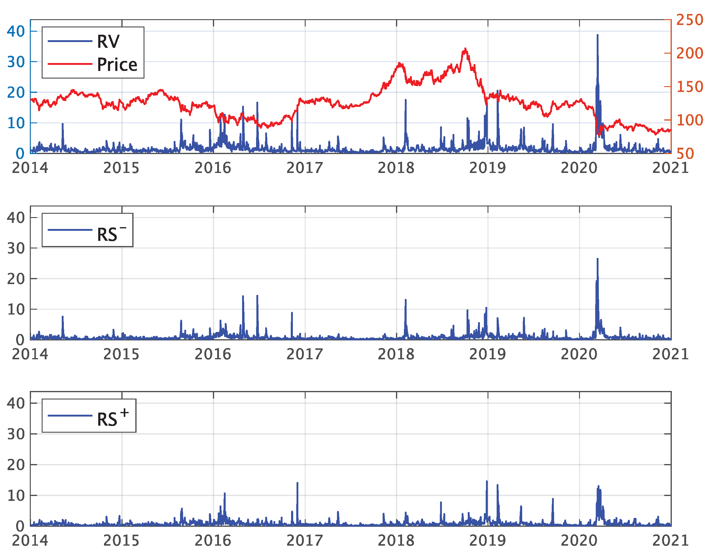
Figure 2.
Volatility spillover networks of realized volatility (RV) and realized semivariance (RS) using NET and net pairwise spillover index.
Figure 2.
Volatility spillover networks of realized volatility (RV) and realized semivariance (RS) using NET and net pairwise spillover index.

Figure 3.
Total volatility spillover, spillover asymmetry measure, and robust check for rolling sample.
Figure 3.
Total volatility spillover, spillover asymmetry measure, and robust check for rolling sample.


Table 1.
Sectors included in the TOPIX-17 series and their symbols.
| Symbol | Sector | Symbol | Sector |
|---|---|---|---|
| Food | Food | IT | Information/Communications/Services/Others |
| Enrg | Energy Resources | ElGs | Electricity/Gas |
| Cnst | Construction/Materials | Tras | Transportation/Logistics |
| Matr | Materials/Chemicals | Whol | Trading/Wholesale |
| Medi | Pharmaceuticals | Reta | Retail |
| Cars | Automobiles/Transportation Equipment | Bank | Banks |
| Stel | Steel/Non-Ferrous | Fina | Finance (excluding banks) |
| Mach | Machinery | Real | Real Estate |
| ElEq | Electric/Precision Machinery |
Table 2.
Descriptive statistics for 17 sectors’ indices’ realized volatility and realized semivariance.
Table 2.
Descriptive statistics for 17 sectors’ indices’ realized volatility and realized semivariance.
| Pre-COVID-19 period (1 January 2014–21 February 2020) | |||||||||||||||||
| Food | Enrg | Cnst | Matr | Medi | Cars | Stel | Mach | ElEq | IT | ElGs | Tras | Whol | Reta | Bank | Fina | Real | |
| Mean | 0.66 | 1.51 | 0.64 | 0.62 | 0.86 | 0.83 | 1.11 | 0.88 | 0.77 | 0.61 | 1.12 | 0.63 | 0.63 | 0.57 | 1.18 | 1.12 | 1.20 |
| Std.dev | 1.03 | 1.70 | 1.09 | 1.04 | 1.28 | 1.58 | 1.52 | 1.36 | 1.38 | 1.09 | 1.27 | 0.98 | 1.08 | 0.92 | 2.20 | 1.96 | 2.00 |
| Max | 20.94 | 20.51 | 20.46 | 20.42 | 27.91 | 27.53 | 29.75 | 24.86 | 27.39 | 22.62 | 23.34 | 21.68 | 18.31 | 16.25 | 31.58 | 32.38 | 33.53 |
| Min | 0.06 | 0.18 | 0.05 | 0.06 | 0.09 | 0.07 | 0.11 | 0.08 | 0.06 | 0.04 | 0.09 | 0.05 | 0.06 | 0.05 | 0.08 | 0.07 | 0.09 |
| Skewness | 9.22 | 5.19 | 9.21 | 8.99 | 9.88 | 9.28 | 8.27 | 8.01 | 9.32 | 9.77 | 8.10 | 11.06 | 8.79 | 8.88 | 8.07 | 8.09 | 8.70 |
| Kurtosis | 136.45 | 40.55 | 123.45 | 124.94 | 162.59 | 118.62 | 115.75 | 100.70 | 133.45 | 148.08 | 112.73 | 185.62 | 112.24 | 120.20 | 86.78 | 91.56 | 103.51 |
| COVID-19 period (25 February 2020–31 December 2020) | |||||||||||||||||
| Food | Enrg | Cnst | Matr | Medi | Cars | Stel | Mach | ElEq | IT | ElGs | Tras | Whol | Reta | Bank | Fina | Real | |
| Mean | 0.99 | 2.15 | 1.48 | 1.10 | 1.43 | 1.63 | 2.35 | 1.41 | 1.39 | 1.09 | 1.50 | 1.81 | 1.18 | 1.02 | 1.60 | 1.69 | 2.59 |
| Std.dev | 1.90 | 3.99 | 2.88 | 2.49 | 2.97 | 3.21 | 3.62 | 2.91 | 3.30 | 2.58 | 2.55 | 3.10 | 2.48 | 2.08 | 3.05 | 3.45 | 4.58 |
| Max | 19.76 | 38.77 | 28.69 | 28.67 | 35.72 | 36.36 | 38.31 | 32.14 | 38.43 | 28.36 | 19.80 | 31.04 | 29.63 | 20.41 | 32.31 | 37.90 | 46.70 |
| Min | 0.07 | 0.26 | 0.10 | 0.09 | 0.15 | 0.14 | 0.23 | 0.12 | 0.12 | 0.07 | 0.21 | 0.06 | 0.10 | 0.07 | 0.09 | 0.08 | 0.20 |
| Skewness | 5.67 | 5.27 | 5.64 | 7.40 | 7.67 | 6.83 | 5.69 | 6.63 | 7.34 | 6.87 | 4.33 | 5.36 | 7.47 | 5.64 | 6.00 | 6.32 | 5.46 |
| Kurtosis | 46.14 | 38.41 | 44.53 | 72.10 | 79.94 | 64.25 | 47.74 | 60.80 | 72.90 | 62.16 | 24.55 | 41.52 | 76.88 | 43.36 | 51.42 | 56.83 | 42.93 |
| Pre-COVID-19 period (1 January 2014–21 February 2020) | |||||||||||||||||
| Food | Enrg | Cnst | Matr | Medi | Cars | Stel | Mach | ElEq | IT | ElGs | Tras | Whol | Reta | Bank | Fina | Real | |
| Mean | 0.34 | 0.77 | 0.33 | 0.32 | 0.44 | 0.43 | 0.58 | 0.45 | 0.40 | 0.32 | 0.57 | 0.32 | 0.32 | 0.29 | 0.59 | 0.56 | 0.61 |
| Std.dev | 0.69 | 1.06 | 0.75 | 0.71 | 0.86 | 1.04 | 1.03 | 0.93 | 0.95 | 0.74 | 0.76 | 0.67 | 0.76 | 0.60 | 1.39 | 1.24 | 1.15 |
| Max | 16.81 | 14.42 | 16.71 | 16.86 | 21.78 | 20.79 | 23.54 | 20.84 | 21.10 | 17.26 | 15.23 | 16.99 | 15.48 | 13.43 | 28.43 | 25.55 | 21.29 |
| Min | 0.01 | 0.04 | 0.02 | 0.01 | 0.03 | 0.02 | 0.03 | 0.03 | 0.02 | 0.02 | 0.05 | 0.02 | 0.02 | 0.02 | 0.03 | 0.03 | 0.04 |
| Skewness | 13.47 | 6.87 | 12.68 | 12.98 | 14.34 | 12.36 | 12.31 | 12.23 | 12.90 | 12.96 | 9.88 | 15.90 | 13.10 | 11.89 | 12.43 | 12.32 | 10.66 |
| Kurtosis | 266.18 | 69.01 | 220.12 | 243.04 | 301.40 | 197.29 | 223.92 | 217.28 | 230.74 | 239.71 | 153.87 | 338.72 | 225.70 | 205.85 | 201.34 | 205.15 | 153.34 |
| COVID-19 period (25 February 2020–31 December 2020) | |||||||||||||||||
| Food | Enrg | Cnst | Matr | Medi | Cars | Stel | Mach | ElEq | IT | ElGs | Tras | Whol | Reta | Bank | Fina | Real | |
| Mean | 0.51 | 1.11 | 0.75 | 0.57 | 0.72 | 0.80 | 1.17 | 0.71 | 0.71 | 0.56 | 0.76 | 0.90 | 0.60 | 0.53 | 0.80 | 0.84 | 1.34 |
| Std.dev | 1.13 | 2.43 | 1.65 | 1.53 | 1.75 | 1.83 | 2.04 | 1.65 | 1.96 | 1.52 | 1.39 | 1.75 | 1.50 | 1.21 | 1.75 | 2.07 | 3.06 |
| Max | 13.70 | 26.54 | 19.69 | 20.73 | 23.42 | 24.07 | 24.81 | 20.68 | 26.03 | 19.11 | 14.44 | 21.22 | 20.22 | 14.13 | 21.67 | 27.07 | 38.85 |
| Min | 0.03 | 0.10 | 0.03 | 0.02 | 0.05 | 0.03 | 0.09 | 0.05 | 0.04 | 0.03 | 0.05 | 0.03 | 0.02 | 0.03 | 0.03 | 0.03 | 0.03 |
| Skewness | 7.54 | 7.13 | 7.43 | 10.08 | 9.64 | 9.21 | 7.30 | 8.23 | 9.55 | 8.57 | 5.64 | 7.45 | 9.78 | 7.16 | 8.09 | 9.19 | 8.66 |
| Kurtosis | 80.04 | 65.37 | 76.62 | 126.91 | 120.05 | 111.61 | 77.39 | 92.70 | 117.63 | 96.11 | 45.47 | 79.18 | 122.98 | 71.86 | 88.18 | 110.08 | 98.49 |
| RS+ | Pre-COVID-19 period (1 January 2014–21 February 2020) | ||||||||||||||||
| Food | Enrg | Cnst | Matr | Medi | Cars | Stel | Mach | ElEq | IT | ElGs | Tras | Whol | Reta | Bank | Fina | Real | |
| Mean | 0.32 | 0.74 | 0.31 | 0.30 | 0.42 | 0.41 | 0.54 | 0.42 | 0.37 | 0.29 | 0.55 | 0.31 | 0.31 | 0.27 | 0.59 | 0.55 | 0.59 |
| Std.dev | 0.45 | 0.99 | 0.48 | 0.46 | 0.57 | 0.73 | 0.69 | 0.65 | 0.60 | 0.46 | 0.63 | 0.44 | 0.48 | 0.40 | 1.15 | 1.02 | 1.16 |
| Max | 6.24 | 14.62 | 6.63 | 6.19 | 7.22 | 10.79 | 8.74 | 11.73 | 7.11 | 5.83 | 11.09 | 7.68 | 7.74 | 6.16 | 20.30 | 15.42 | 25.03 |
| Min | 0.02 | 0.05 | 0.02 | 0.01 | 0.04 | 0.03 | 0.04 | 0.03 | 0.02 | 0.01 | 0.02 | 0.02 | 0.01 | 0.01 | 0.02 | 0.03 | 0.03 |
| Skewness | 6.03 | 7.39 | 7.56 | 6.84 | 6.08 | 7.99 | 4.96 | 7.83 | 6.33 | 6.60 | 6.36 | 7.67 | 6.98 | 6.75 | 8.72 | 8.45 | 13.12 |
| Kurtosis | 54.72 | 83.17 | 83.08 | 67.22 | 53.65 | 88.92 | 39.10 | 99.47 | 56.83 | 62.13 | 75.40 | 92.96 | 76.52 | 72.05 | 108.68 | 98.73 | 240.48 |
| COVID-19 period (25 February 2020–31 December 2020) | |||||||||||||||||
| Food | Enrg | Cnst | Matr | Medi | Cars | Stel | Mach | ElEq | IT | ElGs | Tras | Whol | Reta | Bank | Fina | Real | |
| Mean | 0.47 | 1.04 | 0.73 | 0.53 | 0.71 | 0.83 | 1.18 | 0.69 | 0.67 | 0.53 | 0.74 | 0.90 | 0.58 | 0.49 | 0.81 | 0.86 | 1.25 |
| Std.dev | 0.88 | 1.89 | 1.38 | 1.11 | 1.39 | 1.60 | 1.86 | 1.39 | 1.51 | 1.17 | 1.30 | 1.56 | 1.13 | 1.00 | 1.49 | 1.65 | 1.99 |
| Max | 6.90 | 13.04 | 11.37 | 10.43 | 12.30 | 12.29 | 14.88 | 12.58 | 12.70 | 10.49 | 9.11 | 13.82 | 9.81 | 9.97 | 10.83 | 11.23 | 14.72 |
| Min | 0.03 | 0.06 | 0.05 | 0.04 | 0.04 | 0.04 | 0.12 | 0.06 | 0.05 | 0.04 | 0.06 | 0.03 | 0.04 | 0.03 | 0.03 | 0.02 | 0.05 |
| Skewness | 4.39 | 4.26 | 4.53 | 5.54 | 5.59 | 5.05 | 4.50 | 5.51 | 5.42 | 5.61 | 4.07 | 4.48 | 5.28 | 5.52 | 4.20 | 4.18 | 3.65 |
| Kurtosis | 25.50 | 23.09 | 27.54 | 39.94 | 40.66 | 32.23 | 28.02 | 40.38 | 37.36 | 40.41 | 21.64 | 28.77 | 37.55 | 42.61 | 23.73 | 22.44 | 18.10 |
Table 3.
Total spillover table based on realized volatility during pre-COVID-19 and COVID-19 periods.
Table 3.
Total spillover table based on realized volatility during pre-COVID-19 and COVID-19 periods.
| Pre-COVID-19 period (1 January 2014–21 February 2020) | ||||||||||||||||||
| Food | Enrg | Cnst | Matr | Medi | Cars | Stel | Mach | ElEq | IT | ElGs | Tras | Whol | Reta | Bank | Fina | Real | FROM | |
| Food | 7.9 | 2.4 | 6.6 | 6.5 | 6.5 | 6.1 | 5.9 | 5.9 | 6.3 | 6.7 | 5.2 | 6.4 | 5.9 | 6.9 | 4.5 | 5.7 | 4.6 | 92.1 |
| Enrg | 5.0 | 15.6 | 5.7 | 6.0 | 5.1 | 5.2 | 6.0 | 7.1 | 6.2 | 5.6 | 3.8 | 4.7 | 6.2 | 5.0 | 4.1 | 4.8 | 3.9 | 84.4 |
| Cnst | 6.5 | 2.6 | 7.2 | 6.8 | 5.9 | 6.3 | 6.1 | 6.4 | 6.6 | 6.6 | 5.1 | 6.2 | 6.2 | 6.5 | 4.8 | 5.7 | 4.6 | 92.8 |
| Matr | 6.4 | 2.9 | 6.8 | 7.2 | 6.1 | 6.2 | 6.2 | 6.6 | 6.8 | 6.5 | 4.9 | 6.1 | 6.1 | 6.4 | 4.8 | 5.7 | 4.3 | 92.8 |
| Medi | 6.9 | 2.5 | 6.4 | 6.6 | 7.7 | 6.0 | 6.1 | 6.1 | 6.5 | 6.6 | 4.9 | 6.3 | 6.0 | 6.6 | 4.7 | 5.7 | 4.3 | 92.3 |
| Cars | 6.3 | 2.5 | 6.6 | 6.5 | 5.7 | 7.1 | 6.1 | 6.3 | 6.6 | 6.2 | 4.8 | 5.9 | 6.2 | 6.1 | 5.5 | 6.3 | 5.1 | 92.9 |
| Stel | 6.3 | 3.0 | 6.6 | 6.6 | 5.9 | 6.3 | 7.6 | 6.7 | 6.7 | 6.3 | 4.7 | 5.9 | 6.3 | 6.0 | 5.0 | 5.8 | 4.4 | 92.4 |
| Mach | 6.1 | 3.4 | 6.7 | 6.8 | 5.8 | 6.3 | 6.5 | 7.3 | 6.9 | 6.4 | 4.5 | 5.8 | 6.3 | 5.9 | 4.9 | 5.9 | 4.5 | 92.7 |
| ElEq | 6.3 | 2.9 | 6.7 | 6.8 | 6.0 | 6.3 | 6.4 | 6.7 | 7.0 | 6.5 | 4.6 | 6.1 | 6.2 | 6.1 | 5.0 | 5.9 | 4.5 | 93.0 |
| IT | 6.7 | 2.6 | 6.7 | 6.7 | 6.2 | 6.0 | 6.0 | 6.3 | 6.5 | 7.4 | 5.1 | 6.2 | 6.0 | 6.6 | 4.7 | 5.7 | 4.5 | 92.6 |
| ElGs | 6.8 | 2.2 | 6.7 | 6.3 | 5.9 | 5.9 | 5.8 | 5.6 | 5.9 | 6.6 | 9.6 | 6.5 | 5.6 | 7.1 | 4.3 | 5.1 | 4.1 | 90.4 |
| Tras | 6.8 | 2.3 | 6.7 | 6.7 | 6.3 | 6.1 | 6.0 | 6.0 | 6.4 | 6.5 | 5.3 | 7.3 | 6.1 | 6.6 | 4.9 | 5.6 | 4.4 | 92.7 |
| Whol | 6.3 | 3.0 | 6.6 | 6.6 | 5.8 | 6.4 | 6.3 | 6.5 | 6.6 | 6.3 | 4.7 | 6.1 | 7.4 | 6.0 | 5.2 | 5.9 | 4.5 | 92.6 |
| Reta | 7.0 | 2.4 | 6.8 | 6.6 | 6.3 | 6.0 | 5.8 | 5.9 | 6.3 | 6.8 | 5.7 | 6.3 | 5.8 | 8.0 | 4.6 | 5.3 | 4.4 | 92.0 |
| Bank | 5.8 | 2.4 | 6.1 | 6.2 | 5.4 | 6.8 | 6.0 | 6.0 | 6.2 | 5.7 | 4.2 | 5.7 | 6.1 | 5.6 | 8.7 | 7.1 | 5.9 | 91.3 |
| Fina | 6.2 | 2.5 | 6.3 | 6.4 | 5.8 | 6.7 | 6.1 | 6.3 | 6.4 | 6.1 | 4.3 | 5.7 | 6.1 | 5.6 | 6.2 | 7.5 | 5.8 | 92.5 |
| Real | 6.0 | 2.5 | 6.2 | 5.9 | 5.4 | 6.6 | 5.5 | 6.0 | 6.0 | 5.9 | 4.1 | 5.6 | 5.8 | 5.7 | 6.3 | 6.9 | 9.6 | 90.4 |
| TO | 101.3 | 42.0 | 104.3 | 104.0 | 94.3 | 99.2 | 96.8 | 100.6 | 102.8 | 101.3 | 75.6 | 95.6 | 97.0 | 98.7 | 79.6 | 93.1 | 73.6 | Total: 91.8 |
| NET | 9.2 | −42.4 | 11.4 | 11.2 | 2.0 | 6.3 | 4.4 | 7.9 | 9.8 | 8.7 | −14.8 | 2.9 | 4.4 | 6.8 | −11.7 | 0.6 | −16.7 | |
| COVID-19 period (25 February 2020–31 December 2020) | ||||||||||||||||||
| Food | Enrg | Cnst | Matr | Medi | Cars | Stel | Mach | ElEq | IT | ElGs | Tras | Whol | Reta | Bank | Fina | Real | FROM | |
| Food | 6.4 | 6.1 | 6.1 | 6.2 | 5.5 | 5.9 | 5.5 | 6.4 | 6.4 | 6.4 | 4.8 | 5.3 | 6.0 | 5.7 | 6.1 | 5.8 | 5.2 | 93.6 |
| Enrg | 5.6 | 9.4 | 6.0 | 5.9 | 5.0 | 5.8 | 5.8 | 6.3 | 6.3 | 6.2 | 4.1 | 4.8 | 5.9 | 5.1 | 6.9 | 5.8 | 4.9 | 90.6 |
| Cnst | 6.0 | 6.3 | 6.3 | 6.2 | 5.4 | 6.1 | 5.8 | 6.5 | 6.4 | 6.3 | 4.5 | 5.1 | 6.0 | 5.6 | 6.3 | 5.9 | 5.4 | 93.7 |
| Matr | 6.2 | 5.8 | 6.1 | 6.4 | 5.6 | 6.0 | 5.6 | 6.4 | 6.4 | 6.4 | 4.5 | 5.2 | 6.1 | 5.7 | 6.2 | 5.9 | 5.4 | 93.6 |
| Medi | 6.3 | 5.3 | 6.1 | 6.3 | 6.3 | 6.0 | 5.5 | 6.4 | 6.4 | 6.3 | 4.9 | 5.2 | 6.2 | 5.6 | 5.9 | 5.9 | 5.4 | 93.7 |
| Cars | 6.0 | 5.9 | 6.2 | 6.2 | 5.5 | 6.4 | 5.9 | 6.4 | 6.3 | 6.2 | 4.7 | 5.2 | 6.0 | 5.5 | 6.2 | 5.9 | 5.3 | 93.6 |
| Stel | 5.9 | 6.0 | 6.1 | 6.0 | 5.3 | 6.2 | 6.6 | 6.4 | 6.1 | 5.9 | 4.6 | 5.2 | 6.0 | 5.3 | 6.6 | 6.1 | 5.6 | 93.4 |
| Mach | 6.1 | 6.1 | 6.2 | 6.3 | 5.6 | 6.1 | 5.8 | 6.6 | 6.4 | 6.3 | 4.5 | 5.1 | 6.1 | 5.6 | 6.3 | 5.9 | 5.3 | 93.4 |
| ElEq | 6.1 | 6.2 | 6.2 | 6.3 | 5.6 | 6.0 | 5.6 | 6.5 | 6.6 | 6.5 | 4.4 | 5.0 | 6.1 | 5.7 | 6.2 | 5.8 | 5.3 | 93.4 |
| IT | 6.2 | 6.4 | 6.1 | 6.3 | 5.5 | 5.8 | 5.4 | 6.5 | 6.6 | 6.8 | 4.3 | 5.0 | 6.1 | 5.8 | 6.2 | 5.8 | 5.2 | 93.2 |
| ElGs | 6.2 | 6.1 | 6.2 | 6.2 | 5.5 | 6.0 | 5.6 | 6.3 | 6.2 | 6.3 | 6.1 | 5.2 | 5.9 | 5.5 | 6.0 | 5.9 | 5.0 | 93.9 |
| Tras | 6.2 | 5.6 | 6.0 | 6.2 | 5.4 | 6.0 | 5.6 | 6.1 | 6.0 | 6.1 | 5.0 | 6.4 | 5.9 | 5.8 | 6.1 | 5.9 | 5.5 | 93.6 |
| Whol | 6.1 | 6.0 | 6.1 | 6.2 | 5.6 | 5.9 | 5.7 | 6.4 | 6.4 | 6.3 | 4.6 | 5.2 | 6.4 | 5.6 | 6.2 | 5.9 | 5.3 | 93.6 |
| Reta | 6.1 | 6.4 | 6.2 | 6.2 | 5.3 | 5.8 | 5.5 | 6.4 | 6.4 | 6.6 | 4.4 | 5.2 | 6.0 | 6.2 | 6.2 | 5.7 | 5.3 | 93.8 |
| Bank | 5.9 | 6.9 | 6.0 | 6.2 | 5.2 | 6.1 | 5.9 | 6.3 | 6.1 | 6.1 | 4.2 | 5.2 | 5.9 | 5.2 | 7.5 | 6.2 | 5.3 | 92.5 |
| Fina | 6.0 | 5.9 | 6.0 | 6.2 | 5.4 | 6.0 | 5.9 | 6.3 | 6.2 | 6.1 | 4.6 | 5.2 | 6.0 | 5.3 | 6.7 | 6.5 | 5.5 | 93.5 |
| Real | 6.0 | 5.5 | 6.1 | 6.1 | 5.3 | 5.9 | 6.0 | 6.2 | 6.1 | 6.1 | 4.8 | 5.5 | 5.9 | 5.7 | 6.1 | 6.2 | 6.4 | 93.6 |
| TO | 96.9 | 96.6 | 97.6 | 99.0 | 86.7 | 95.6 | 91.0 | 102.0 | 100.6 | 100.2 | 73.1 | 82.7 | 95.8 | 88.7 | 100.3 | 94.8 | 85.0 | Total: 93.3 |
| NET | 3.3 | 6.0 | 3.9 | 5.4 | −7.0 | 2.0 | −2.4 | 8.6 | 7.2 | 7.0 | −20.9 | −10.9 | 2.2 | −5.1 | 7.9 | 1.3 | −8.6 | |
Notes: The numbers in bold italics are the spillover itself and total spillover. The numbers in italics in NET are the negative values.
Table 4.
Total spillover table based on negative realized semivariance during pre-COVID-19 and COVID-19 periods.
Table 4.
Total spillover table based on negative realized semivariance during pre-COVID-19 and COVID-19 periods.
| Pre-COVID-19 period (1 January 2014–21 February 2020) | ||||||||||||||||||
| Food | Enrg | Cnst | Matr | Medi | Cars | Stel | Mach | ElEq | IT | ElGs | Tras | Whol | Reta | Bank | Fina | Real | FROM | |
| Food | 7.3 | 3.0 | 6.4 | 6.4 | 6.3 | 6.0 | 5.9 | 6.0 | 6.1 | 6.4 | 5.5 | 6.3 | 5.8 | 6.5 | 5.2 | 6.1 | 4.8 | 92.7 |
| Enrg | 5.0 | 12.2 | 5.8 | 6.1 | 5.4 | 5.4 | 6.2 | 7.0 | 6.4 | 5.6 | 4.4 | 4.7 | 6.0 | 5.1 | 4.9 | 5.4 | 4.4 | 87.8 |
| Cnst | 6.2 | 3.4 | 6.8 | 6.5 | 5.8 | 6.2 | 6.2 | 6.3 | 6.4 | 6.3 | 5.3 | 5.9 | 6.0 | 6.2 | 5.2 | 6.1 | 5.1 | 93.2 |
| Matr | 6.1 | 3.6 | 6.5 | 6.8 | 5.9 | 6.2 | 6.2 | 6.4 | 6.5 | 6.3 | 5.1 | 6.0 | 5.9 | 6.1 | 5.1 | 6.1 | 4.9 | 93.2 |
| Medi | 6.5 | 3.3 | 6.2 | 6.4 | 7.3 | 5.9 | 6.1 | 6.2 | 6.3 | 6.4 | 5.2 | 6.3 | 5.9 | 6.2 | 5.2 | 6.0 | 4.8 | 92.7 |
| Cars | 6.0 | 3.3 | 6.4 | 6.3 | 5.7 | 6.9 | 6.1 | 6.2 | 6.4 | 6.1 | 5.1 | 5.8 | 6.2 | 5.9 | 5.8 | 6.5 | 5.3 | 93.1 |
| Stel | 5.9 | 3.8 | 6.4 | 6.5 | 5.9 | 6.2 | 7.1 | 6.6 | 6.5 | 6.1 | 5.1 | 5.8 | 6.1 | 5.8 | 5.3 | 6.2 | 4.9 | 92.9 |
| Mach | 5.9 | 4.2 | 6.4 | 6.5 | 5.9 | 6.1 | 6.4 | 6.9 | 6.6 | 6.2 | 5.0 | 5.7 | 6.1 | 5.8 | 5.2 | 6.1 | 4.9 | 93.1 |
| ElEq | 5.9 | 3.8 | 6.4 | 6.6 | 5.9 | 6.2 | 6.3 | 6.6 | 6.8 | 6.2 | 4.9 | 5.9 | 6.1 | 5.8 | 5.4 | 6.2 | 5.1 | 93.2 |
| IT | 6.3 | 3.4 | 6.5 | 6.5 | 6.1 | 6.0 | 6.1 | 6.3 | 6.3 | 7.0 | 5.2 | 6.0 | 5.9 | 6.3 | 5.2 | 6.1 | 4.9 | 93.0 |
| ElGs | 6.5 | 3.1 | 6.4 | 6.1 | 5.8 | 5.9 | 5.9 | 5.8 | 5.8 | 6.2 | 8.6 | 6.3 | 5.6 | 6.5 | 4.7 | 5.8 | 5.0 | 91.4 |
| Tras | 6.5 | 2.9 | 6.3 | 6.3 | 6.2 | 6.0 | 5.9 | 5.9 | 6.2 | 6.3 | 5.6 | 7.1 | 5.9 | 6.3 | 5.4 | 6.0 | 5.0 | 92.9 |
| Whol | 5.9 | 3.7 | 6.3 | 6.2 | 5.7 | 6.4 | 6.2 | 6.3 | 6.4 | 6.1 | 5.0 | 5.9 | 7.1 | 5.7 | 5.7 | 6.3 | 5.1 | 92.9 |
| Reta | 6.7 | 3.1 | 6.5 | 6.4 | 6.1 | 6.0 | 5.9 | 6.0 | 6.1 | 6.5 | 5.7 | 6.2 | 5.7 | 7.4 | 5.0 | 5.8 | 4.9 | 92.6 |
| Bank | 5.8 | 3.3 | 6.0 | 5.9 | 5.6 | 6.6 | 5.9 | 5.9 | 6.2 | 5.9 | 4.5 | 5.9 | 6.2 | 5.5 | 8.0 | 6.9 | 5.9 | 92.0 |
| Fina | 6.0 | 3.2 | 6.3 | 6.2 | 5.8 | 6.4 | 6.1 | 6.2 | 6.3 | 6.1 | 4.8 | 5.8 | 6.1 | 5.6 | 6.1 | 7.1 | 5.7 | 92.9 |
| Real | 5.7 | 3.2 | 6.2 | 5.9 | 5.5 | 6.3 | 5.8 | 6.0 | 6.1 | 5.8 | 4.9 | 5.7 | 5.9 | 5.5 | 6.2 | 6.8 | 8.6 | 91.4 |
| TO | 96.9 | 54.3 | 101.0 | 100.8 | 93.6 | 97.9 | 97.1 | 99.6 | 100.7 | 98.7 | 81.2 | 94.1 | 95.4 | 94.8 | 85.8 | 98.3 | 80.7 | Total: 92.4 |
| NET | 4.2 | −33.5 | 7.9 | 7.7 | 0.9 | 4.8 | 4.2 | 6.6 | 7.4 | 5.7 | −10.2 | 1.2 | 2.5 | 2.3 | −6.2 | 5.3 | −10.6 | |
| COVID-19 period (25 February 2020–31 December 2020) | ||||||||||||||||||
| Food | Enrg | Cnst | Matr | Medi | Cars | Stel | Mach | ElEq | IT | ElGs | Tras | Whol | Reta | Bank | Fina | Real | FROM | |
| Food | 6.4 | 5.0 | 6.1 | 6.1 | 5.7 | 5.8 | 5.9 | 6.1 | 6.2 | 6.3 | 5.0 | 5.6 | 6.0 | 5.9 | 6.0 | 6.0 | 5.6 | 93.6 |
| Enrg | 5.1 | 10.1 | 5.9 | 5.6 | 4.9 | 5.9 | 6.4 | 6.3 | 6.5 | 6.0 | 3.9 | 4.5 | 5.7 | 5.0 | 7.7 | 5.9 | 4.6 | 89.9 |
| Cnst | 6.0 | 5.3 | 6.4 | 6.1 | 5.6 | 6.0 | 6.3 | 6.3 | 6.3 | 6.3 | 4.6 | 5.2 | 6.0 | 5.6 | 6.3 | 6.1 | 5.6 | 93.6 |
| Matr | 6.0 | 4.9 | 6.1 | 6.3 | 5.9 | 6.0 | 5.9 | 6.3 | 6.3 | 6.3 | 4.8 | 5.4 | 6.1 | 5.7 | 6.2 | 6.2 | 5.6 | 93.7 |
| Medi | 6.1 | 4.5 | 6.1 | 6.2 | 6.4 | 6.0 | 5.8 | 6.2 | 6.3 | 6.2 | 5.0 | 5.6 | 6.1 | 5.7 | 6.0 | 6.2 | 5.6 | 93.6 |
| Cars | 5.9 | 5.1 | 6.2 | 6.1 | 5.7 | 6.3 | 6.2 | 6.3 | 6.3 | 6.2 | 4.8 | 5.3 | 6.1 | 5.6 | 6.2 | 6.1 | 5.7 | 93.7 |
| Stel | 5.8 | 5.5 | 6.3 | 6.0 | 5.5 | 6.2 | 6.8 | 6.3 | 6.2 | 6.0 | 4.6 | 5.2 | 6.0 | 5.5 | 6.4 | 6.1 | 5.6 | 93.2 |
| Mach | 5.8 | 5.6 | 6.2 | 6.1 | 5.7 | 6.1 | 6.2 | 6.5 | 6.3 | 6.3 | 4.6 | 5.3 | 6.0 | 5.5 | 6.4 | 6.1 | 5.4 | 93.5 |
| ElEq | 5.9 | 5.6 | 6.1 | 6.2 | 5.7 | 6.0 | 6.0 | 6.3 | 6.5 | 6.4 | 4.6 | 5.2 | 6.1 | 5.6 | 6.3 | 6.1 | 5.4 | 93.5 |
| IT | 5.9 | 5.7 | 6.1 | 6.2 | 5.6 | 5.9 | 6.0 | 6.3 | 6.4 | 6.6 | 4.6 | 5.1 | 6.0 | 5.6 | 6.3 | 6.1 | 5.4 | 93.4 |
| ElGs | 6.1 | 5.0 | 6.1 | 5.9 | 5.5 | 5.8 | 5.9 | 6.0 | 6.0 | 6.1 | 6.8 | 5.5 | 5.9 | 5.8 | 5.9 | 6.0 | 5.5 | 93.2 |
| Tras | 6.3 | 4.5 | 6.0 | 6.1 | 5.8 | 5.9 | 5.8 | 6.1 | 6.0 | 6.1 | 5.3 | 6.5 | 5.9 | 6.0 | 5.8 | 6.0 | 5.8 | 93.5 |
| Whol | 6.0 | 5.1 | 6.1 | 6.1 | 5.7 | 6.0 | 6.0 | 6.2 | 6.3 | 6.2 | 5.0 | 5.4 | 6.3 | 5.7 | 6.2 | 6.2 | 5.7 | 93.7 |
| Reta | 6.2 | 5.3 | 6.1 | 6.0 | 5.6 | 5.8 | 6.0 | 6.1 | 6.2 | 6.3 | 4.9 | 5.6 | 6.0 | 6.4 | 6.0 | 5.9 | 5.7 | 93.6 |
| Bank | 5.6 | 6.3 | 6.0 | 6.1 | 5.5 | 6.0 | 6.2 | 6.3 | 6.3 | 6.1 | 4.6 | 5.1 | 6.0 | 5.2 | 7.3 | 6.2 | 5.2 | 92.7 |
| Fina | 5.9 | 5.2 | 6.1 | 6.2 | 5.7 | 6.0 | 6.0 | 6.3 | 6.3 | 6.3 | 4.8 | 5.3 | 6.1 | 5.4 | 6.4 | 6.4 | 5.6 | 93.6 |
| Real | 6.1 | 4.4 | 6.1 | 6.1 | 5.7 | 6.0 | 6.1 | 6.0 | 6.1 | 6.1 | 5.1 | 5.6 | 6.2 | 6.0 | 5.8 | 6.1 | 6.5 | 93.5 |
| TO | 94.7 | 83.2 | 97.6 | 97.1 | 89.7 | 95.4 | 96.8 | 99.4 | 99.9 | 99.1 | 76.4 | 85.0 | 96.3 | 89.9 | 99.8 | 97.4 | 87.9 | Total: 93.3 |
| NET | 1.1 | −6.7 | 4.0 | 3.5 | −3.9 | 1.7 | 3.6 | 5.9 | 6.4 | 5.7 | −16.9 | −8.5 | 2.6 | −3.6 | 7.2 | 3.8 | −5.6 | |
Notes: The numbers in bold italics are the spillover itself and total spillover. The numbers in italics in NET are the negative values.
Table 5.
Total spillover table based on positive realized semivariance during pre-COVID-19 and COVID-19 periods.
Table 5.
Total spillover table based on positive realized semivariance during pre-COVID-19 and COVID-19 periods.
| Pre-COVID-19 period (1 January 2014–21 February 2020) | ||||||||||||||||||
| Food | Enrg | Cnst | Matr | Medi | Cars | Stel | Mach | ElEq | IT | ElGs | Tras | Whol | Reta | Bank | Fina | Real | FROM | |
| Food | 11.3 | 1.1 | 6.7 | 6.4 | 7.0 | 5.9 | 4.5 | 4.3 | 6.4 | 7.9 | 5.2 | 7.1 | 5.5 | 8.7 | 2.7 | 4.3 | 4.9 | 88.7 |
| Enrg | 4.1 | 26.3 | 5.2 | 6.1 | 4.5 | 4.7 | 5.5 | 6.4 | 6.1 | 5.5 | 2.5 | 4.2 | 6.5 | 4.1 | 2.3 | 3.7 | 2.4 | 73.7 |
| Cnst | 6.4 | 1.2 | 8.5 | 7.7 | 6.1 | 6.6 | 5.7 | 6.3 | 7.3 | 7.1 | 4.5 | 6.8 | 6.5 | 6.6 | 3.5 | 5.1 | 4.0 | 91.5 |
| Matr | 6.0 | 1.5 | 7.7 | 8.8 | 6.3 | 6.5 | 5.9 | 6.8 | 7.8 | 6.9 | 4.0 | 6.5 | 6.6 | 6.3 | 3.7 | 5.2 | 3.5 | 91.2 |
| Medi | 7.4 | 1.2 | 6.9 | 7.1 | 10.2 | 5.8 | 5.1 | 5.2 | 7.1 | 7.5 | 4.6 | 6.6 | 5.9 | 7.6 | 3.4 | 4.8 | 3.5 | 89.8 |
| Cars | 5.8 | 1.3 | 7.1 | 7.1 | 5.6 | 8.6 | 6.0 | 6.8 | 7.6 | 6.3 | 3.7 | 6.0 | 6.5 | 5.6 | 4.4 | 6.6 | 4.8 | 91.4 |
| Stel | 5.8 | 1.7 | 7.1 | 7.1 | 5.4 | 6.8 | 9.8 | 7.3 | 7.5 | 6.3 | 3.8 | 5.6 | 7.1 | 5.4 | 4.0 | 5.3 | 4.1 | 90.2 |
| Mach | 5.0 | 1.9 | 7.4 | 7.9 | 5.6 | 7.2 | 7.0 | 8.9 | 8.2 | 6.3 | 3.2 | 5.7 | 7.0 | 5.1 | 3.9 | 6.0 | 3.8 | 91.1 |
| ElEq | 6.0 | 1.5 | 7.3 | 7.7 | 6.1 | 7.0 | 6.1 | 7.0 | 8.6 | 7.1 | 3.9 | 6.1 | 6.4 | 6.1 | 3.6 | 5.6 | 4.0 | 91.4 |
| IT | 7.2 | 1.4 | 7.3 | 7.1 | 6.6 | 6.0 | 5.0 | 5.4 | 7.3 | 9.4 | 4.9 | 7.0 | 6.1 | 7.5 | 3.2 | 4.7 | 4.0 | 90.6 |
| ElGs | 7.8 | 0.8 | 7.0 | 6.0 | 6.2 | 5.5 | 4.7 | 3.9 | 6.0 | 7.6 | 14.3 | 7.1 | 5.1 | 8.4 | 3.0 | 3.8 | 3.1 | 85.7 |
| Tras | 7.3 | 1.1 | 7.5 | 7.2 | 6.6 | 6.1 | 5.0 | 5.2 | 6.8 | 7.5 | 5.1 | 9.0 | 6.3 | 7.2 | 3.6 | 4.8 | 3.7 | 91.0 |
| Whol | 6.0 | 1.8 | 7.3 | 7.4 | 6.0 | 6.6 | 6.4 | 6.6 | 7.3 | 6.9 | 3.8 | 6.4 | 8.9 | 5.8 | 3.7 | 5.4 | 3.7 | 91.1 |
| Reta | 8.3 | 1.2 | 7.2 | 6.9 | 7.1 | 5.6 | 4.6 | 4.6 | 6.6 | 8.0 | 5.7 | 7.0 | 5.6 | 10.5 | 3.0 | 4.1 | 4.1 | 89.5 |
| Bank | 4.5 | 1.1 | 6.2 | 6.7 | 5.2 | 7.2 | 6.2 | 6.1 | 6.5 | 5.3 | 3.4 | 5.6 | 5.9 | 4.7 | 13.0 | 9.0 | 3.5 | 87.0 |
| Fina | 5.4 | 1.3 | 6.6 | 6.8 | 5.7 | 7.7 | 5.7 | 6.6 | 7.1 | 6.0 | 3.2 | 5.7 | 6.2 | 5.0 | 6.4 | 9.3 | 5.3 | 90.7 |
| Real | 7.0 | 1.2 | 6.9 | 6.2 | 5.3 | 7.1 | 4.9 | 5.5 | 6.1 | 6.6 | 3.1 | 5.8 | 5.9 | 6.3 | 3.4 | 6.0 | 12.8 | 87.2 |
| TO | 100.2 | 21.0 | 111.5 | 111.4 | 95.1 | 102.4 | 88.2 | 94.1 | 111.6 | 108.6 | 64.6 | 99.2 | 99.2 | 100.3 | 57.6 | 84.5 | 62.5 | Total: 88.9 |
| NET | 11.6 | −52.8 | 20.0 | 20.2 | 5.4 | 11.0 | −2.0 | 3.0 | 20.1 | 17.9 | −21.1 | 8.2 | 8.0 | 10.7 | −29.4 | −6.2 | −24.7 | |
| RS+ | COVID-19 period (25 February 2020–31 December 2020) | |||||||||||||||||
| Food | Enrg | Cnst | Matr | Medi | Cars | Stel | Mach | ElEq | IT | ElGs | Tras | Whol | Reta | Bank | Fina | Real | FROM | |
| Food | 8.3 | 6.9 | 6.5 | 7.5 | 6.1 | 5.7 | 3.7 | 7.1 | 7.5 | 8.6 | 4.5 | 4.6 | 6.3 | 6.4 | 5.0 | 3.8 | 1.4 | 91.7 |
| Enrg | 7.2 | 10.7 | 6.2 | 6.7 | 4.7 | 5.3 | 4.4 | 6.3 | 6.6 | 7.6 | 5.9 | 4.8 | 6.0 | 5.6 | 5.4 | 4.3 | 2.4 | 89.3 |
| Cnst | 7.0 | 7.5 | 7.3 | 7.2 | 5.4 | 6.1 | 4.6 | 7.3 | 7.4 | 8.0 | 4.1 | 4.2 | 6.3 | 6.0 | 5.3 | 4.1 | 2.2 | 92.7 |
| Matr | 7.5 | 6.9 | 6.7 | 7.7 | 6.1 | 6.0 | 4.1 | 7.7 | 7.9 | 8.7 | 3.6 | 4.1 | 6.4 | 6.2 | 5.2 | 3.8 | 1.5 | 92.3 |
| Medi | 7.7 | 6.2 | 6.5 | 7.3 | 8.3 | 6.2 | 4.2 | 7.9 | 7.6 | 8.0 | 4.0 | 3.8 | 6.5 | 5.6 | 4.8 | 4.0 | 1.3 | 91.7 |
| Cars | 7.2 | 6.6 | 6.9 | 7.1 | 6.0 | 7.5 | 5.0 | 7.6 | 7.3 | 7.8 | 3.6 | 4.3 | 6.4 | 5.6 | 5.1 | 4.1 | 2.0 | 92.5 |
| Stel | 6.2 | 6.5 | 7.0 | 6.5 | 5.0 | 6.8 | 7.6 | 6.9 | 6.4 | 6.1 | 3.6 | 4.6 | 6.3 | 4.7 | 6.2 | 5.7 | 3.9 | 92.4 |
| Mach | 7.0 | 6.9 | 7.0 | 7.4 | 6.2 | 6.4 | 4.6 | 8.1 | 7.8 | 8.2 | 3.6 | 3.6 | 6.6 | 5.9 | 5.1 | 3.8 | 1.7 | 91.9 |
| ElEq | 7.1 | 6.9 | 6.9 | 7.6 | 5.8 | 5.7 | 4.2 | 7.7 | 8.3 | 9.0 | 3.4 | 3.6 | 6.4 | 6.4 | 5.2 | 3.8 | 1.8 | 91.7 |
| IT | 7.6 | 7.0 | 6.6 | 7.6 | 5.9 | 5.4 | 3.7 | 7.8 | 8.4 | 9.8 | 3.4 | 3.8 | 6.5 | 6.9 | 5.1 | 3.3 | 1.3 | 90.2 |
| ElGs | 8.2 | 7.4 | 6.2 | 7.4 | 6.5 | 5.5 | 3.4 | 7.1 | 7.2 | 8.5 | 7.0 | 4.7 | 6.1 | 6.2 | 4.5 | 3.4 | 0.9 | 93.0 |
| Tras | 7.8 | 6.5 | 6.0 | 6.9 | 5.4 | 6.0 | 4.2 | 6.4 | 6.4 | 7.4 | 4.4 | 7.4 | 6.4 | 5.9 | 5.7 | 4.7 | 2.5 | 92.6 |
| Whol | 7.2 | 6.8 | 6.6 | 7.2 | 5.9 | 6.0 | 4.5 | 7.5 | 7.2 | 8.0 | 3.6 | 4.5 | 8.2 | 5.9 | 5.2 | 3.9 | 1.8 | 91.8 |
| Reta | 7.7 | 6.9 | 6.6 | 7.6 | 6.2 | 5.7 | 3.5 | 7.6 | 8.0 | 9.1 | 3.9 | 4.2 | 6.6 | 7.5 | 4.9 | 3.1 | 1.2 | 92.5 |
| Bank | 6.8 | 7.1 | 6.4 | 6.7 | 4.7 | 5.7 | 5.1 | 6.4 | 6.4 | 7.3 | 3.3 | 5.3 | 6.0 | 5.1 | 8.3 | 5.8 | 3.5 | 91.7 |
| Fina | 6.8 | 7.2 | 6.1 | 6.5 | 4.7 | 5.6 | 5.3 | 6.2 | 6.2 | 6.8 | 3.7 | 5.3 | 5.7 | 4.4 | 7.2 | 7.5 | 4.7 | 92.5 |
| Real | 5.7 | 8.8 | 5.9 | 5.5 | 3.4 | 5.1 | 5.7 | 5.5 | 5.6 | 6.1 | 4.7 | 5.3 | 5.0 | 4.3 | 6.7 | 7.7 | 9.0 | 91.0 |
| TO | 114.8 | 112.1 | 104.1 | 112.8 | 88.0 | 93.3 | 70.2 | 112.8 | 113.8 | 125.2 | 63.1 | 70.6 | 99.6 | 91.3 | 86.6 | 69.4 | 34.0 | Total: 91.9 |
| NET | 23.1 | 22.7 | 11.4 | 20.5 | −3.8 | 0.8 | −22.2 | 20.9 | 22.1 | 35.0 | −29.9 | −22.0 | 7.7 | −1.2 | −5.1 | −23.1 | −57.1 | |
Notes: The numbers in bold italics are the spillover itself and total spillover. The numbers in italics in NET are the negative values.
Publisher’s Note: MDPI stays neutral with regard to jurisdictional claims in published maps and institutional affiliations. |
© 2022 by the authors. Licensee MDPI, Basel, Switzerland. This article is an open access article distributed under the terms and conditions of the Creative Commons Attribution (CC BY) license (https://creativecommons.org/licenses/by/4.0/).
Share and Cite
MDPI and ACS Style
Shigemoto, H.; Morimoto, T. Volatility Spillover among Japanese Sectors in Response to COVID-19. J. Risk Financial Manag. 2022, 15, 480. https://doi.org/10.3390/jrfm15100480
AMA Style
Shigemoto H, Morimoto T. Volatility Spillover among Japanese Sectors in Response to COVID-19. Journal of Risk and Financial Management. 2022; 15(10):480. https://doi.org/10.3390/jrfm15100480
Chicago/Turabian StyleShigemoto, Hideto, and Takayuki Morimoto. 2022. "Volatility Spillover among Japanese Sectors in Response to COVID-19" Journal of Risk and Financial Management 15, no. 10: 480. https://doi.org/10.3390/jrfm15100480