
The Interplay between COVID-19 and the Economy in Canada


1
Department of Mathematics, Federal University of Santa Catarina, Florianópolis 88040-900, Brazil
2
Department of Mathematics and Statistics, McMaster University, Hamilton, ON L8S 4K1, Canada
3
School of Computing and Data Science, Wentworth Institute of Technology, Boston, MA 02115, USA
4
Mathematics Department, Khalifa University, Abu Dhabi 127788, United Arab Emirates
*
Author to whom correspondence should be addressed.
J. Risk Financial Manag. 2022, 15(10), 476; https://doi.org/10.3390/jrfm15100476
Submission received: 5 August 2022
/
Revised: 4 October 2022
/
Accepted: 6 October 2022
/
Published: 18 October 2022
(This article belongs to the Special Issue Systemic Recovery: Lessons from COVID-19, Modeling, Analysis, and Policy Implications)
Abstract
:We propose a generalized susceptible-exposed-infected-removed (SEIR) model to track COVID-19 in Canadian provinces, taking into account the impact of the pandemics on unemployment. The model is based on a network representing provinces, where the contact between individuals from different locations is defined by a data-driven mixing matrix. Moreover, we use time-dependent parameters to account for the dynamical evolution of the disease incidence, as well as changes in the rates of hospitalization, intensive care unit (ICU) admission, and death. Unemployment is accounted for as a reduction in the social interaction, which translates into smaller transmission parameters. Conversely, the model assumes that higher proportions of infected individuals reduce overall economic activity and therefore increase unemployment. We tested the model using publicly available sources and found that it is able to reproduce the reported data with remarkable in-sample accuracy. We also tested the model’s ability to make short-term out-of-sample forecasts and found it very satisfactory, except in periods of rapid changes in behavior. Finally, we present long-term predictions for both epidemiological and economic variables under several future vaccination scenarios.
1. Introduction
Since the seminal work of Kermack and McKendrick (1927), mathematical models have played an essential role in the modeling of infectious diseases dynamics. Susceptible-infected-removed (SIR) and susceptible-exposed-infected-removed (SEIR) models are two of the most widely used models designed to describe the spread of an emerging pathogen in a susceptible population (Keeling and Rohani 2008), and since the beginning of the coronavirus disease 2019 (COVID-19) pandemic, several SEIR-type models have been proposed to describe the spread of the SARS-CoV-2 virus (Albani et al. 2021; Amaku et al. 2021; Calvetti et al. 2020b; Campos et al. 2021; Chen et al. 2022; Gatto et al. 2020; Grimm et al. 2021; Lyra et al. 2020).
During the first outbreak of COVID-19, several catastrophic predictions (regarding the number of deaths and hospital occupations) have emerged worldwide (Ioannidis et al. 2020). Such predictions were based, in general, on over-simplistic models and poor data. Fortunately, such forecasted scenarios did not materialize, although more accurate predictions were urgently needed. To address the need of better data, public authorities from different countries have improved their data collection, data organization, and data sharing services on, among others, COVID-19 testing, infections, deaths, and hospitalizations. This allowed the World Health Organization (WHO) to track the worldwide evolution of the COVID-19 pandemics and let researchers test their models with real data1.
To improve the forecast ability of SEIR-type models, a series of features were incorporated into the original models. One of them, inspired by the widely implemented mobility restrictions, was the spatial spread of the pathogen. Some works considered the spatial dynamics based on the distance between neighborhoods (Albani et al. 2021; Calvetti et al. 2020b; Gatto et al. 2020; Wu et al. 2020), others used mobility data based on mobile phone information (Alleman et al. 2021; Candido et al. 2020; Coelho et al. 2020; Kishore et al. 2021). Another important feature incorporated into the model was the different levels of disease severity, commonly grouped as asymptomatic, mild, severe, and critical (Albani et al. 2021; Amaku et al. 2021; Campos et al. 2021). Such severity was highly dependent on demographic factors, such as age and sex (Bhopal and Bhopal 2020; CDC 2020; Jin et al. 2020; Verity et al. 2020; WHO 2020), which were also considered in some models (Albani et al. 2021; Cartocci et al. 2021; Grimm et al. 2021), given their importance in the prediction of hospital and intensive care unit (ICU) usage. The performance and forecast accuracy of such SEIR-type models were also considerably improved when some parameters were considered as time-dependent (Albani et al. 2021, 2022; Calvetti et al. 2020a, 2020b). This allowed the models to incorporate regime changes in the dynamics caused, for example, by the emergence of new variants or treatments that change the pathogen transmission pattern and mortality rates, as well as a variety of public health measures, ranging from lockdowns to vaccination.
These modeling improvements resulted in a series of theoretical and data-driven numerical experiments to quantitatively access the performance of different techniques used to control COVID-19 outbreaks. For example, SEIR-type models were used to quantify the efficacy of different non-pharmaceutical measures, such as lockdowns and the use of masks (Alleman et al. 2021; Eikenberry et al. 2020; IHME COVID-19 Forecasting Team 2020; Kishore et al. 2021). Epidemiological models were also used to predict the impact of vaccination strategies in the population (Albani et al. 2021b; Amaku et al. 2021; Libotte et al. 2020), as well as to evaluate the effects of underreporting of infections and deaths (Albani et al. 2021a; Aronna et al. 2022; Chen et al. 2022; Kupek 2021; McMahan et al. 2021; Saberi et al. 2020). It was also possible to access the role of socioeconomic programs in the mitigation of outbreaks (Albani et al. 2021).
Concerning the calibration of epidemiological models, different techniques were applied, including deterministic (optimization) and stochastic (Bayesian inference) methods. The main issue in calibration is overfitting, where a model fits observed data well, but has serious difficulty in predicting future scenarios. This phenomenon is caused by the interplay between uncertainties and noise associated with the data collection and the use of an excessive number of model parameters. To address this problem, different techniques can be applied depending on the calibration method. In general, deterministic models use some sort of regularization, for example, à la Tikhonov (Engl et al. 1996; Scherzer et al. 2008). In the context of stochastic methods, inference techniques based on statistical analysis are used to incorporate such uncertainties into the solution (Gamerman and Lopes 2006; Migon et al. 2014; Somersalo and Kapio 2004), at the expense of being more computationally intensive than deterministic methods. In the context of the calibration of epidemiological models for COVID-19, deterministic methods were used, for example, by Albani et al. (2021); Chen et al. (2022); He et al. (2020); Leonov et al. (2021); Ramadijanti and Basuki (2020), and stochastic techniques were used in Calvetti et al. (2020a, 2020b); Gianfelice et al. (2022); Lyra et al. (2020); Monod et al. (2021); Unwin et al. (2020).
The economic impacts of the COVID-19 pandemic were also widely studied under different perspectives. Some studies (Fernández-Villaverde and Jones 2020; Maliszewska et al. 2020; OECD 2020) compiled and summarized the evidence of the impact on traditional economic measures, such as GDP, employment, and trade, whereas others (Ashraf 2020; Storm 2021) used statistical methods to quantify the effects of different non-pharmaceutical interventions and compare their effectiveness across multiple countries. As informative as these empirically-based studies can be, one difficulty with this approach is the lack of an underlying model governing the dynamics of both the pandemic and the economy, which makes it particularly challenging for them to make reliable medium- and long-term forecasts.
A different strand of the literature, represented for example by Acemoglu et al. (2021); Alvarez et al. (2021); Bayraktar et al. (2021) focused instead on the design of optimal policies, typically by extending an SEIR-like model through the introduction of an optimal control problem. This type of approach, however, faces the difficulty of unrealistic modeling assumptions, such as the definition of an agreed-upon objective function for a central planner, with well-understood effects of the pandemic on the economy, and the ability to execute precise controls, such as having exact time-dependent fractions of the population under a lockdown regime. A related strand, represented for example by Eichenbaum et al. (2021); Farboodi et al. (2021), seeks to endogenize behavior, such as physical distancing by having rational individuals decide on their level of social interaction based on the probability of becoming infected. As in traditional macroeconomic models, these decisions are made with the view of maximizing the utility of consumption over an infinite time horizon, with the resulting model suffering from the same deficiencies as mainstream dynamic stochastic general equilibrium (DSGE) models, including a lack of heterogeneity, perfect foresight, and instability of the solution path.
As an alternative to either a purely empirical approach or an unrealistic theoretical approach, the work presented, for example, in Kemp-Benedict (2020), Cruz-Aponte and Caraballo-Cueto (2021), and Balmford et al. (2020), combined an epidemiological SEIR-like model with a more phenomenological macroeconomic model. Along similar lines, we highlight the contribution of Góes and Gallo (2021), to which our paper is closely related. Their central idea is to relate a key economic variable, namely the unemployment rate u, with one key epidemiological variable, namely the positivity rate i, through a stylized model of the form
The motivation for this model is that, absent the pandemic, the unemployment rate converges to a long-term equilibrium , whereas an increase in the number of infected people leads to higher unemployment through the interaction term in Equation (1) with a constant . This is meant to include all the effects of the pandemic on the economy, both direct and indirect, such as sick people not being able to work, slowdowns in economic activity caused by lockdown measures, business closures, and the like. Conversely, an increase in unemployment rate leads to a decrease in the number of infected people through the term in (2) with a constant . Again, this is meant to encapsulate all the effects of the economy on the pandemic, both direct and indirect, such as lower mobility when unemployed people stay at home, as well as overall lower contact and transmission during lockdown periods and corresponding lower economic activity. The equilibrium points for (1) and (2) are
namely, an endemic equilibrium with and a non-endemic one with . Góes and Gallo (2021) then chose the parameter based on estimates available in the literature for the contact, recovery, and death rates for COVID-19 in the US, and estimated the parameter based on the observed reduction in the basic reproductive number when containment measures were introduced. The parameters and were estimated using the time series for the unemployment and positivity rates for the US, whereas the parameter was chosen to be compatible with conventional estimates of long-term unemployment for the US economy. They simulated the model with these parameter values and observed convergence to the endemic equilibrium with unemployment close to and a positivity rate close to . Finally, Góes and Gallo (2021) simulated a stochastic version of (1) and (2) and compared it with the observed dynamics for these two variables, obtaining relatively good agreement from the start of the pandemic until November 2020, using data available prior to the acceptance date of the article in December 2020.
Our work can be characterized as an extension of the model of Góes and Gallo (2021) applied to the Canadian economy. On the epidemiological side, we replaced Equation (1) with a fully developed SEIR-type model with each compartment stratified by location, age, and employment status. On the economic side, we replaced Equation (2) with equations describing the flows between the employed and unemployed groups in each compartment. In addition, similar to Góes and Gallo (2021), we estimated a relationship between the unemployment rate and economic output, known as Okun’s law, before and throughout the pandemic, in order to convert the labor market information into predictions of GDP for each province in Canada.
More specifically, in comparison to the existing literature, the main contributions of the present article are the following:
- An epidemiological model that accounts for spatial spread, time-dependent parameters, different levels of disease severity, vaccination, age-range dependency, and labor status of those of working age.
- Model parameters that are calibrated from the daily Canadian provincial reports on COVID-19 infections, hospitalizations, admissions to ICU, deaths, and monthly labor status.
- An explicit connection between the pandemic and the economy through labor market dynamics.
The calibrated model is able to provide accurate predictions and presents a remarkable fit to the observed data, including periods of rapidly varying policies, both economic and epidemiological. Toward the end of the article, we present long-term predictions for the future evolution of COVID-19 and its economic impact based on a number of scenarios for vaccination and loss of immunity.
2. The Model
We present the model under a general formulation considering different locations ℓ, age groups a and employment status s. For the empirical application, will correspond to different Canadian provinces and territories, to the age groups 0 to 19, 20 to 69, and over 69 years old, and corresponding to employed and unemployed individuals.
Thus, for each location and age range, the population is distributed into the following compartments: susceptible (), vaccinated (), exposed but not infective (), infective and mildly ill (), infected and hospitalized (), infected and in an intensive care unit (), and recovered (). The deceased individuals are denoted by D, regardless if they came from the employed or unemployed group. Before describing the disease dynamics in more detail, let us introduce a vector notation as follows. For each employment status s, let denote the number of susceptible individuals in the age range a and location ℓ and define
where A denotes the number of age groups and L denotes the number of different locations. That is to say, is an -row vector with components, whose first A components are the number of susceptible individuals of different ages in the first location, the next A components are the number of susceptible individuals of different ages in the second location, and so forth. The vectors , , , , , , and are defined similarly. We also introduce the tensor product
The schematic representation of the model for each location and age range in Equations (7)–(21) can be found in Figure 1.
As in a regular SEIR model, susceptible individuals can become exposed upon contact with infective ones, whereas exposed individuals become infective after an incubation time. Each mildly ill infective individual can recover, become hospitalized, or die. Hospitalized infected individuals can recover or develop more severe symptoms and be admitted to an ICU. Those individuals in the ICU can only recover or die. We also admit the possibility of reinfection, i.e., individuals in the vaccinated and recovered compartments can become susceptible after a while. In principle, individuals in each compartment could move between employment statuses, but we assume that there is no possibility of becoming employed or unemployed while in the hospital. That is to say, only the individuals in the compartments (i.e., susceptible, vaccinated, exposed, mildly infective, and recovered) can change the employment status.
Accordingly, the detailed epidemiological model is defined as follows:
The matrices , , and are the transmission parameters for the mildly ill, hospitalized, and in intensive care infective classes, respectively, taking into account the age group and location for each class. More specifically, , , and are time-dependent symmetric matrices, where , A is the number of age groups and L is the number of locations. The matrix is defined as,
where , for , are symmetric matrices and , for , are time-dependent scalar quantities. Notice that the entries for the matrices could, in principle, be estimated from information about transmission between different age groups in different provinces. Because this is not available in the data, we make the simplifying assumption these entries are identical for a given , which is equivalent to assuming that, given a pair of provinces , the probability of transmission is uniform across age groups. Specifically, for each , all the entries of are given by
with , and is the probability of an individual from place i to meet someone from place j. The parameters depend on the distance between the locations i and j, and are estimated from the daily reports of infections. Again, to reduce the number of parameters, we assume that can only take five different values when , depending on whether the distance between the centers2 of i and j falls is less than Km, from to Km, from to Km, from to Km, or larger than Km3. The matrices and satisfy and , where a and b are scale parameters that reduce the transmission rate amongst the hospitalized and in ICU individuals.
Most of the remaining parameters in the model are column vectors corresponding to specific transition rates between compartments for each age group and location. Namely, the vectors and are the hospitalization and ICU admission rates, respectively. The vectors , , and are the recovery rates of mildly ill, hospitalized, and intensive care-infected individuals, respectively. The vectors and are the mortality rates of those outside a hospital and in the ICU, respectively. Notice that we assume that individuals outside a hospital or in a critical state (in an ICU) can die since in Canada a number of deaths occurred outside hospitals as pointed in WHO (2020). The vector denotes the vaccination rate. The vector has components equal to the inverse of the mean time of incubation for each age group and location. Similarly, the vector r has components equal to the inverse of the mean time that someone vaccinated or recovered from the disease becomes susceptible again, for each age group and location. Finally, the vectors and denote, respectively, the transition rates from unemployed to employed status and vice-versa. Individuals outside the working age receive the label e and, in these cases, the corresponding components for the rates and are set to 0.
We also assume that unemployed individuals have a smaller risk of getting infected, and this is represented by the scalar parameter , with corresponding to the case of unemployed individuals having no risk of becoming infected. This means that, when someone is unemployed, it is expected that they will take public transportation less often, as they are not going to work, and will spend more time at home, which means a sort of self-isolation. Since hospitalized individuals are isolated, there is no difference in interacting with employed or unemployed individuals in the hospital or ICU.
Regarding the labor market, observe that the total number of employed and unemployed individuals in the population can be obtained from the other variables of the model as follows:
In other words, we assume that the vectors and in the epidemiological model in Equations (7)–(21), are given by
where the parameters and represent the baseline transition rates into the employed and unemployed groups, whereas the parameters and represent the additional sensitivity of these rates with respect to new infections. The parameter is the Canadian population size in 2020, i.e., 38.0 million. This parameter is used to scale up the new infections represented by , , in comparison to the proportions of employed and unemployed individuals that have higher magnitudes.
3. Estimation Procedure
We begin with the model parameters in Equations (7)–(21) that can be obtained directly from available data without resourcing to any sophisticated estimation procedure, namely
Starting with the vector parameters, the rates of hospitalization , ICU admission , and mortality rate are treated as time-dependent and estimated according to the available information for each Canadian province, whereas the remaining parameters in (29) are treated as constant and calibrated to values from the related literature.
More precisely, is assumed to be identical for all age groups and labor statuses. It is set such that is equal to the number of hospitalizations on day t. The rate is defined similarly, using the daily reports of ICU admissions and hospitalizations in the ℓ-th place. The death rate is set to for all locations and age groups, following Abate et al. (2020). The death rate is also assumed to be identical for all age groups and labor status. It is defined to be such that is equal to the reported deaths in the ℓth place on day t. Thus, is equal to the reported deaths on day t, in the ℓ-th place, minus , for all age groups.
The rates of recovery of mildly ill, hospitalized, and intensive care individuals are set, respectively, as days(WHO 2020), days(Guan et al. 2020), and days(Grasselli et al. 2020) for all locations and age groups. The incubation time is set to be constant and equal to 5.1 days for all age groups and locations, which is the median time found by Lauer et al. (2020). Similarly, the rate r is also assumed to be constant and equal for all age groups and locations. For the baseline calibration of the model, we set , whereas we use chose different values for the scenario analysis presented later. It is now well documented that vaccinated and recovered individuals can lose their immunity, and seroprevalence decreases with time. However, this time can vary dramatically depending on a series of factors (Goldberg et al. 2021; Levin et al. 2021; Spellberg et al. 2021). In the simulations that follow, setting is equivalent to assuming that 360 days is the mean time vaccinated and recovered individuals return to the susceptible condition.
Finally, the vector denotes the vaccination rate and is proportional to the number of individuals receiving the second dose daily in each age group and location times , which represents the efficacy of the vaccines used in Canada. Other ways of including spatial information into SEIR-like models can be found in (Albani et al. 2021; Calvetti et al. 2020b; Gatto et al. 2020; Keeling and Rohani 2008).
Moving on to scalar parameters, similarly to Albani et al. (2021), the quantities a and b are set to and . As we do not have epidemiological information accounting unemployment, for simplicity, we set , which means that transmission among unemployed individuals is half the transmission among employed people, due to the self-isolation caused by not going to work. Whereas small perturbations around this value for do not affect the qualitative behavior of the model in a significant way, a systematic sensitivity analysis of the model for different values of this parameter is not feasible, as it requires the repeated re-estimation and simulation of a high-dimensional model with large computational costs. In the event that disease incidence data for employed and unemployed groups become available, the parameter could be estimated similarly to the other parameters in the model.
The remaining model parameters need to be estimated from publicly available daily numbers of COVID-19 infections through a so-called maximum a posteriori technique from Bayesian Inference Somersalo and Kapio (2004). We denote by the following vector of unknown parameters:
where is the initial population of mildly infective individuals in the ℓth location, regardless of age group and employment status, and and are the parameters introduced in (23).
We then use available data on newly infected individuals to estimate the vector as follows. Let us assume that the daily number of new infections in the ℓ-th location, denoted by , is Poisson-distributed with parameter , where denotes the number of exposed and not infective individuals in the ℓ-th location, regardless of age group or employment status. More precisely, using the notation introduced in (5), we have that
The logarithm of the likelihood function4 is then
with T the number of elements in the time series. We use non-overlapping consecutive intervals of 20 daily observations each to estimate the parameters in a time-dependent manner.
The prior density of the vector of parameters is assumed to be Gaussian, with the mean given by a set of a priori parameters , and covariance equals the identity matrix. Hence, the logarithm of the posterior density is proportional to
The value can be identified with the regularization parameter in a Tikhonov-type regularization (Engl et al. 1996). The estimated parameters are obtained by minimizing assuming that , for in (22). The time-dependent coefficients are then estimated in a separate step, i.e., after the estimation of , as follows: for each , for , minimize the following functional:
where . The functional F is proportional to the posterior density of , given , and .
Regarding the initial conditions for the model, notice that, using the notation introduced in (5), the parameters in (30) are given by
Once the parameters are estimated as explained above, we obtain each of the based on the proportion of the population for each age range and labor status. The remaining initial conditions for the model are set as follows: is set to the proportion of the Canadian population in the ℓth location at the ath age minus the sum of the initial conditions for the other compartments with the same values for s,a, and ℓ. If or 3, . If , then is multiplied by the proportions of unemployed and employed individuals. Apart from the infective compartments, the initial conditions for all the other compartments are set to zero.
The estimation of the parameters and are performed similarly, but using data about changes in employment status instead. Firstly, we have to adjust the labor market data to be used within the epidemiological model since for each location ℓ we have monthly totals of employed and unemployed individuals and daily reports of new infections. As the model does not consider natural births and deaths, which means that the sum of all the compartments is constant in time, we divide the monthly numbers of employed and unemployed by the corresponding monthly labor force (i.e., the sum of employed and unemployed individuals). The resulting numbers are then multiplied by the proportion of individuals of working age in the same location for the year 2020. Moreover, to transform the monthly reports into daily data, we interpolate them linearly. The resulting series are then used to estimate the daily and , for and . Since the number of unknowns for each day is four and the daily data are two, a moving window of four consecutive days is used. For such four consecutive days, we assume that the parameter values are constant in time. If and represent the adjusted daily reports and and denote the solution of the model in Equations (26) and (27), using the daily reported infections for the ℓth place, and using as initial condition the adjusted reported employed and unemployed numbers, we obtain the parameters by minimizing the functional
for and , where the parameters are estimated in the previous step5.
4. Numerical Results
In this section, we present the results for the calibration of the model in Equations (7)–(21) using real data. We also perform backtesting by considering the accuracy of short-term model predictions.
4.1. Model Calibration
We use the 7-day moving average version of the time series of daily reported infections, hospitalizations, ICU admissions, deaths, and second vaccine doses inoculated from the 13 Canadian provinces and territories, provided by Esri Canada.6 We also use demographic data provided by Statistics Canada.7 The labor data consists of the provincial monthly total number of unemployed individuals also provided by Statistics Canada.8 The time series considered in this numerical example correspond to the period from 19 February 2020 to 28 February 2022.
Starting with the epidemiological parameters, Figure 2 shows the values for the 7-day moving average of the time-dependent parameters for the 6 largest Canadian provinces. As expected, we can observe increases in the values of all the parameters during the successive waves of infections or large outbreaks, as well as other patterns broadly consistent with reported news about the pandemic. For example, while the hospitalization rate exhibited a large peak during the omicron wave in the beginning of 2022, the peaks in death and ICU admissions rates for the same period were similar to those during previous waves of infections. This indicates that omicron caused less severe outcomes than the earlier variants.9
Moving on to the labor market parameters, Figure 3 presents estimated values of the time-dependent parameters , , , and for the six largest Canadian provinces. We can observe in the figure that all six provinces experienced a higher level of activity in the labor market throughout the pandemic, evidenced by larger values of the baseline transition rates , between employed and unemployed groups. Notice also that the estimates for were positive, whereas the estimates for were negative, confirming the intuition that an increase in infections has the overall effect of increasing unemployment, in accordance with the model and results of Góes and Gallo (2021). Finally, observe that this sensitivity of unemployment with respect to new infections only begins to be significant towards the start of 2021, as the level of government emergence support in place during most of 2020 resulted in a very weak direct link between infections and unemployment.
Figure 4 shows the comparison between the 7-day moving average of nationwide daily numbers of infections, deaths, hospitalizations, ICU admissions, fully vaccinated, as well as estimated unemployed individuals and their corresponding model predictions obtained with calibrated parameters.
To compare the model predictions for the number of unemployed individuals with the reported data, we reverse the steps explained in the previous section to transform the data. Namely, we first obtain a prediction for the monthly proportion of unemployed individuals of working age in each location by using the corresponding daily prediction for the first day of each month. Next, we divide these predictions by the proportion of individuals of working age in each location in 2020 to obtain monthly predictions for the unemployment rate in each location and multiply the result by the size of the labor force for that month, using the size of the labor force in February 2022 for simulations past that date. Finally, we aggregate the resulting number of unemployed individuals for the entire country.
As one can see from Figure 4, all the in-sample model predictions were remarkably adherent to the reports, illustrating the model accuracy when all the available data are used to estimate the time-varying parameters. Specifically, the in-sample calibration error, to be defined in detail in the next section, for the period 19 February 2020 to 28 February 2022 was approximately 11%. In practice, of course, one is interested in out-of-sample predictions, so in the next section we investigate the accuracy of the model when only a portion of the available data are used to estimate the parameters, which are then used to make predictions for subsequent periods.
4.2. Backtesting
In order to analyze the forecast capability of the proposed model, we performed a series of backtests. More precisely, we calibrated the model using non-overlapping periods of 20 days each and made out-of-sample predictions 7 days ahead, using the average of the estimated parameter values of the last five days in each period. The comparison between the out-of-sample model predictions and nationwide reports of COVID-19 cases, hospitalizations, ICU admissions, and deaths for some periods can be found in Table 1.
Table 1 also presents the calibration and prediction error, which were evaluated as follows: in both cases, we multiplied by 100 the -norm of the difference between the vectors containing the model predictions and reports of daily COVID-19 infections divided by the -norm of the vector containing the reports. The calibration error refers to the error in the in-sample predictions and the prediction error refers to the error in the out-of-sample predictions. Thus, using the notation from Section 3, both the in-sample (Calib. Error) and the out-of-sample (Predic. Error) errors are evaluated using the following formula:
We considered only the infections in the evaluation of the errors since we used only the reported COVID-19 cases in the model calibration.
Calibration errors were mainly below 5%, whereas prediction errors were mainly below 20%, which is in agreement with other proposed models, such as Albani et al. (2021). This illustrates the efficiency and the accuracy of the proposed model to design short-term predictions regardless if the incidence is increasing, decreasing, or stable.
We also tested the model prediction capability for longer periods. Figure 5 compares 30-day ahead model predictions with reports during different disease incidence trends.
As Figure 5 shows, the model is able to capture the trend in the incidence, extrapolating it for longer periods and providing accurate predictions. The model predictions in the testing set, i.e., the reported data not used in the calibration, are obtained with the average of the estimated parameter values for the last 5 days in the training set, i.e., the dataset used in the calibration. Thus, as long as the observed trend at the end of the training set is kept, the model is able to provide accurate predictions. However, during longer periods, incidence trends can revert, and the model prediction can degenerate as in the predictions for the periods from 19 April to 19 May 2020 and from 1 October to 31 October 2020. Whenever such loss of prediction accuracy occurs, the parameters in the model must be updated. Note that such loss of accuracy in long-term predictions is not unusual due to the nonlinearity and stochastic nature of the phenomena under consideration, as well as the enforcement of new restrictions. For example, since 15 April 2020, international travelers were required to stay in quarantine when entering Canada and since 17 April 2020, air and rail passengers were required to use face masks CIHI (2022); Vogel and Eggertson (2020). Such new rules can be related to the loss of accuracy in the predictions for the period from 19 April to 19 May 2020. In 1 October 2020, stringent containment measures were undertaken in Quebec to control the rise of cases CP24 (2020). Such measures can also be related to the loss of accuracy from 1 October to 31 October 2020.
It is also worth mentioning that we are modeling the COVID-19 outbreak in Canada considering a number of different scales, i.e., different levels of disease severity for each Canadian province or territory, accounting for age range, vaccination, and unemployment. Thus, due to the large complexity of the proposed model and its calibration from real data, we can assert that the performances of the predictions are more than satisfactory.
4.3. Long-Term Predictions
It is by now well known that after recovering from the infection or after vaccination, immunity decreases with time. Such loss of immunity can be caused by a series of reasons, including the emergence of new variants of the SARS-CoV-2, such as the delta and omicron variants, which caused large outbreaks worldwide even in countries with efficient vaccination coverage, such as Canada, the United States, and the United Kingdom. Thus, we assumed that after a period of 360 days, anyone who recovered or who was vaccinated returned to the susceptible compartment.
We considered periodic vaccination campaigns with the following periods, 270, 360, 390, 450, 540, and 720 days. Figure 6, Figure 7 and Figure 8 show the different projections of the evolution of infections, deaths, and unemployed individuals under different vaccination scenarios, using a 10-day average for the time-dependent parameters as of 28 February 2022, namely the end of the calibration period used in Section 4.1.
As can be seen in the graphs, when the vaccination period is shorter than the assumed average time for loss of immunity (namely 360 days), the number of infections rapidly decrease and remain negligible, whereas longer vaccination periods lead to periodic resurgence in infections, with peak numbers comparable to what was observed during the 2020–2022 waves of the pandemic (with the exception of the omicron wave at the start of 2022). Observe that, as the intervals between successive vaccination campaigns increase, the infection waves become less frequent and with larger amplitudes, and similar patterns can be observed in the number of daily deaths. We also observe an increase in the corresponding wave in the monthly unemployment rate as vaccination becomes less frequent, but because of the nonlinear relationship between new infections and the labor market expressed in Equations (26) and (27), their amplitudes first increase and then decrease, with the largest oscillations occurring when the interval between vaccinations is 450 days.
5. Economic Effect
In this section, we analyze the effect of this pandemic on the economy in a manner similar to Góes and Gallo (2021). Namely, we use the following revised version of Okun’s law10:
where Y is the observed GDP, k is the growth rate of GDP output under constant unemployment, is a factor relating changes in unemployment to the growth rate in GDP, and u is the observed unemployment rate.
In order to predict the impact of COVID-19 on the economy, we estimated the parameters using Canadian national data time series. For the unemployment rate u, expressed as a percentage of the labor force, we used quarterly data provided by the OECD11 and computed the differences between consecutive periods to obtain . For GDP growth rate , we used quarterly data provided by the OECD12, expressed as percentage change from the previous period.
Applying the ordinary least square (OLS) regression methods, we estimate theses parameters from the first quarter of 2015 to the first quarter of 2022, using data from the preceding 16 quarters for each estimate. The estimated values of the parameters k and during the pandemic, together with the corresponding standard deviations, can be found in Table 2, whereas the estimates including the previous 5 years can be found in Figure 9.
As we can see in Table 2, the estimated value for the long-term (i.e., prevailing under constant unemployment) quarterly growth rate in output k dropped from 0.51% to 0.26% from the first to second quarters of 2020 (or from 2.07% to 1.06% in terms of annualized growth rates), illustrating the contraction caused by the onset of the pandemic, and subsequently bounced back to around 0.6% (or a 2.4% annualized growth rate) once the economic stimulus measures were in effect, before stabilizing around 0.4% (or a 1.61% annualized growth rate), which is close to the pre-pandemic 5-year average. Similarly, the estimated value for initially increased significantly from 0.71 to 2.74 and then decreased again and stabilized around 1.95, still higher than the pre-pandemic 5-year average of 1.23 but in line with other estimates for Canada and the United States. In other words, the relationship between changes in unemployment and GDP growth first became stronger at the start of the pandemic, before stabilizing towards its previous pattern.
We can now use the results of both the epidemiological model in Equations (7)–(21) and Okun’s law to check for consistency between the model and our different data sources, as well as to make long-term predictions of economic effects. Starting with the Canadian unemployment rate, Figure 10 shows the comparison between the quarterly unemployment rate obtained directly from the OECD dataset and the unemployment rate computed from data from Statistics Canada. To compute the Stats Canada unemployment rate, we first aggregate the provincial monthly data used in the previous section into national quarterly averages and then divide the total number of unemployed individuals by the labor force. As we can see, the Stats Canada unemployment rate is considerably noisier than the OECD unemployment rate, primarily because of seasonal adjustment used by the OECD, which is why we chose this time series to estimate Okun’s law.
Figure 11 shows the comparison between the Stats Canada monthly unemployment rate during the pandemic and the corresponding model predictions for the same period. As expected from the good agreement in the number of unemployed individuals already seen in Figure 4, the unemployment rate predicted by the model is close to the Stats Canada unemployment rate. Accordingly, we can use the model to make the forecasts shown in Figure 11 for the Canadian unemployment rate under different future vaccination scenarios, with a similar pattern as observed for the total number of unemployed individuals in Figure 8.
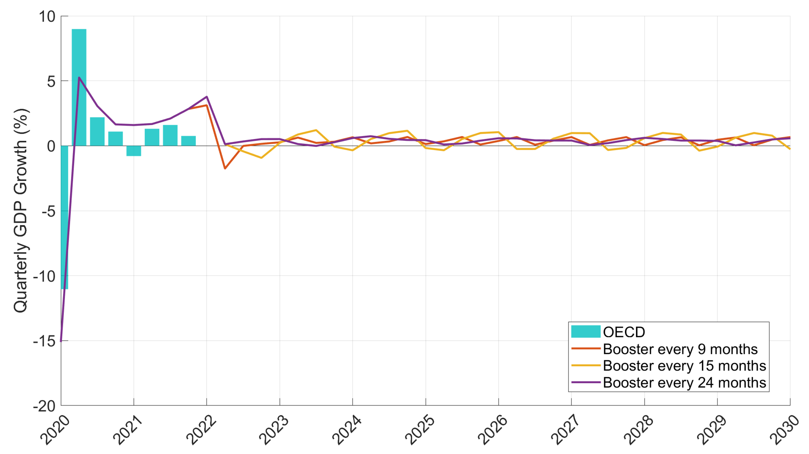
Moving to economic output, in the top panel of Figure 12 we compare the percentage change in quarterly GDP in Canada obtained directly from the OECD dataset with those obtained using data from Stats Canada by calculating the percentage change in quarterly GDP from monthly GDP data.13 As we can observe, these two sources provide nearly identical data, and either can be used in comparisons with model predictions. Next, in the bottom panel of Figure 12, we compare the OECD-reported percentage change in quarterly GDP in Canada and those calculated from the estimated Okun law (34) using quarterly changes in the unemployment rate reported by the OECD as an input. We can see that our estimated Okun’s law fits the historical data relatively well, including during the pandemic. More specifically, we can observe a precipitous drop in the quarterly percentage change of Canadian GDP in 2020 Q2, coinciding with the beginning of the COVID pandemic in Canada. Subsequently, with the financial support from the Canadian government and control of the first wave in 2020 Q3, the percentage change in GDP experienced a large rebound. Following the second wave of transmission, the speed of economic recovery began to slow down again in 2020 Q4 and stabilized at historical levels from 2021 Q1 onward.
Figure 13 shows the predictions of percentage change in quarterly GDP in Canada obtained from the estimated14 Okun’s law (34) using the quarterly changes in unemployment rate predicted by the model as an input. As we can see, the quarterly changes in GDP predicted in this way also fit the data well during the pandemic. Accordingly, we use the model to make forecasts for quarterly growth rates in GDP under different future vaccination scenarios. Unsurprisingly, given the pattern of unemployment observed in Figure 11, we also see a similar behavior for the cycles of GDP growth, namely less frequent vaccination campaigns lead to GDP growth oscillations of increasing periods, but increasing and then decreasing amplitudes.
6. Conclusions and Further Research Directions
In this paper, we developed a combined economic–epidemiological model to investigate the effects of the COVID-19 pandemic in Canada. The epidemiological part of the model consists of an extension of the susceptible-exposed-infected-removed (SEIR) along the lines of Albani et al. (2021), i.e., incorporating time-varying parameters (when applicable), multiple geographic regions (Canadian provinces and territories), and multiple age groups. This last feature was introduced in the model so that we could identify a working age group and establish a link between the pandemic and the economy via unemployment. For this, we further subdivided each compartment in the model into the employed and unemployed sub-compartments and adjusted the epidemiological dynamics accordingly, for example, by assuming that contact rates between individuals in unemployed compartments are lower than in employed ones, reflecting less mobility between home and work as well as less exposure to the general public for those who are unemployed. Crucially, we also assumed that the labor market dynamics were also affected by the pandemic through time-varying transition rates between employment status with an explicit dependence on new infections, along the lines suggested in Góes and Gallo (2021). To explore the economic effects further, we assumed an Okun’s law relationship between the changes in unemployment and GDP, and estimated them before and during the pandemic.
As shown in Figure 4, the calibrated model was able to fit the observed data remarkably well, with an in-sample calibration error of approximately 11% when the entire available dataset was used in the estimation of the parameters. The performance was also satisfactory when shorter periods (20 days) were used in the estimation and we used the model to make predictions 7 days ahead, with calibration errors mainly below 5% and prediction errors mainly below 20%, as shown in Table 1. However, Figure 5 illustrates that, as should be expected, the performance of the model deteriorates when it is used to make longer term (i.e., 30 days ahead) predictions during periods of rapid changes in behavior, and consequently model parameters, such as when new lockdown measures were imposed. Even in these instances, however, periodic re-calibration of the underlying parameters is enough to restore the performance of the model.
With this caveat in mind, we used the model to make long-term predictions (i.e., up to 2030) for COVID-19 under different future scenarios for vaccinations and assuming that loss of immunity occurs on average 360 days after either vaccine or recovery from the disease. Figure 6, Figure 7 and Figure 8 show the predictions for infections, deaths, and unemployed individuals for a variety of scenarios, as an example of how the model can be used by policymakers interested in the design of vaccination campaigns.
Regarding the economic impact, Figure 9 shows that estimates for long-term quarterly growth rate at constant unemployment, namely the parameter k in Okun’s law (34), exhibited a sharp decline at the start of the pandemic, followed by a quick rebound throughout 2020 and a reversion to the pre-pandemic average toward the end of 2021. On the other hand, the response of quarterly growth rates to unemployment, namely the parameter in Okun’s law (34), became stronger at the start of the pandemic and then stabilized at a level higher than the pre-pandemic average. Interestingly, whereas the uncertainty in the estimate of k increased since the start of the pandemic, the uncertainty in the estimate of appears to have decreased.
The links between the labor market and disease dynamics embedded throughout the model, most notably in Equations (26) and (27), allowed us to make the long-term forecasts for unemployment rates, shown in Figure 11, with cycles following a pattern differently from that observed for infections and deaths, namely as the intervals between vaccination campaigns increased, the amplitude of oscillations in unemployment rates first became larger, but eventually began to decrease. This in turn can be converted into long-term forecasts for the GDP growth rates shown in Figure 13.
As mentioned above, we offer these long-term predictions as illustrations of how the model can be used as a tool to aid policy-making, rather than authoritative statements about the future dynamics of these variables. Specifically, what we have in mind is that policy makers should run the model under a variety of plausible parameter values and policy scenarios (e.g., vaccination intervals) to obtain the range of outcomes for the variables of interest, notably deaths and unemployed individuals.
Having explored here a reasonably detailed epidemiological model for Canada, including multiple compartments for different stages of the disease (e.g., moderate, hospitalized, admitted to ICU), as well as age groups and geographic locations, in future work we plan to focus on simpler versions of the model but extend the analysis to a larger number of countries. Specifically, we will consider aggregate national data and a simplified epidemiological structure for a set of representative countries (e.g., USA, United Kingdom, Italy, China, etc.) and explore the differences in the infection–unemployment nexus in the context of a reduced model, which opens up the possibility of analytical results, in addition to the estimation and simulation-based results presented here.
Author Contributions
All the authors contributed equally to the development, the model, and the interpretation of the results. V.A. conducted the estimation and simulation of the epidemiological part of the model and W.P. conducted the estimation and simulation of the economic part of the model. All authors have read and agreed to the published version of the manuscript.
Funding
V.A. acknowledges the financial support from Fundação Butantan and Fundação de Amparo à Pesquisa e Inovação do Estado de Santa Catarina through grant nos. 01/2020 and 00002847/2021, respectively. J.Z. acknowledges the financial support from Khalifa University, CNPq, and Fundação Carlos Chagas Filho de Amparo à Pesquisa do Estado do Rio de Janeiro through grant nos. FSU-2020-09, 307873/2013-7, and E-26/202.927/2017, respectively. M.G. and W.P. acknowledge the financial support from the Natural Sciences and Engineering Research Council of Canada through the Discovery Grants program.
Data Availability Statement
Publicly available datasets were used in this study. All code and data needed to implement the model can be found at https://github.com/viniciusalbani/Covideconomics (accessed on 5 October 2022).
Conflicts of Interest
The authors declare no competing interests.
| 1 | See, for example, covid19.who.int (accessed on 5 October 2022). |
| 2 | Data on air travel distance downloaded 20 November 2020 from https://www.distancefromto.net/ (accessed on 20 November 2020). |
| 3 | For clarity, consider provinces and suppose that the distance between the centers of 1 and 2 is in the same range as the distance between the centers of 2 and 3, say 3000 to 4000 K. We then impose the constraint and estimate using data for both pairs of provinces. This reduces the original 78 parameters , , to the five parameters . |
| 4 | The term 1 inside the argument for the logarithms is added to avoid indefinite values when the number of reported infections is zero. |
| 5 | Notice that, to find the values for j = 1,2,3, we just have to consider the series values for previous dates. |
| 6 | Data downloaded on 15 March 2022 from https://resources-covid19canada.hub.arcgis.com/datasets/provincial-daily-totals/explore (accessed on 15 March 2022). |
| 7 | Data downloaded on 20 Novemver 2020 from https://www.statcan.gc.ca/eng/subjects-start/population_and_demography (accessed on 20 Novemver 2020). |
| 8 | Data downloaded on 1 July 2022 from https://www150.statcan.gc.ca/t1/tbl1/en/tv.action?pid=1410028703 (accessed on 1 July 2022). |
| 9 | In accordance with data in https://www.cdc.gov/coronavirus/2019-ncov/variants/omicron-variant.html (accessed on 20 May 2022). |
| 10 | |
| 11 | Data downloaded on 20 July 2022 from https://data.oecd.org/unemp/unemployment-rate.htm (accessed on 20 July 2022). |
| 12 | Data downloaded on 20 July 2022 from https://data.oecd.org/gdp/quarterly-gdp.htm (accessed on 20 July 2022). |
| 13 | Downloaded on 20 July 2022 from https://www150.statcan.gc.ca/t1/tbl1/en/cv.action?pid=3610043401 (accessed on 20 July 2022). |
| 14 | We use a 12-month average of the time-varying parameters in Okun’s law for these simulations. |
References
- Abate, Semagn Mekonnen, Siraj Ahmed Ali, Bahiru Mantfardo, and Bivash Basu. 2020. Rate of Intensive Care Unit admission and outcomes among patients with coronavirus: A systematic review and Meta-analysis. PLoS ONE 15: e0235653. [Google Scholar] [CrossRef] [PubMed]
- Acemoglu, Daron, Victor Chernozhukov, Iván Werning, and Michael D. Whinston. 2021. Optimal targeted lockdowns in a multigroup sir model. American Economic Review: Insights 3: 487–502. [Google Scholar] [CrossRef]
- Albani, Vinicius V. L., Roseane A. S. Albani, Nara Bobko, Eduardo Massad, and Jorge P. Zubelli. 2021. On the Role of Financial Support Programs in Mitigating the Sars-CoV-2 Spread in Brazil. BMC Public Health 22: 1781. [Google Scholar] [CrossRef] [PubMed]
- Albani, V., R. Albani, E. Massad, and J. Zubelli. 2022. Nowcasting and forecasting COVID-19 waves: The recursive and stochastic nature of transmission. Royal Society Open Science 9: 220489. [Google Scholar] [CrossRef] [PubMed]
- Albani, Vinicius, Jennifer Loria, Eduardo Massad, and Jorge Zubelli. 2021a. COVID-19 Underreporting and its Impact on Vaccination Strategies. BMC Infectious Diseases 21: 1111. [Google Scholar] [CrossRef] [PubMed]
- Albani, Vinicius V. L., Jennifer Loria, Eduardo Massad, and Jorge P. Zubelli. 2021b. The Impact of COVID-19 Vaccination Delay: A Data-Driven Modelling Analysis for Chicago and New York City. Vaccine 39: 6088–6094. [Google Scholar] [CrossRef] [PubMed]
- Albani, Vinicius V. L., Roberto M. Velho, and Jorge P. Zubelli. 2021. Estimating, monitoring, and forecasting COVID-19 epidemics: A spatiotemporal approach applied to NYC data. Scientific Reports 11: 1–15. [Google Scholar] [CrossRef]
- Alleman, Tijs, Jenna Vergeynst, Lander De Visscher, Michiel Rollier, Elena Torfs, Ingmar Nopens, and Jan Baetens. 2021. Assessing the effects of non-pharmaceutical interventions on SARS-CoV-2 transmission in Belgium by means of an extended SEIQRD model and public mobility data. Epidemics 37: 100505. [Google Scholar] [CrossRef]
- Alvarez, Fernando, David Argente, and Francesco Lippi. 2021. A simple planning problem for COVID-19 lock-down, testing, and tracing. American Economic Review: Insights 3: 367–82. [Google Scholar] [CrossRef]
- Amaku, Marcos, Dimas Tadeu Covas, Francisco Antonio Bezerra Coutinho, Raymundo Soares Azevedo, and Eduardo Massad. 2021. Modelling the impact of delaying vaccination against SARS-CoV-2 assuming unlimited vaccine supply. Theoretical Biology and Medical Modelling 18: 1–11. [Google Scholar] [CrossRef]
- Amaku, Marcos, Dimas Tadeu Covas, Francisco Antonio Bezerra Coutinho, Raymundo Soares Azevedo Neto, Claudio Struchiner, Annelies Wilder-Smith, and Eduardo Massad. 2021. Modelling the test, trace and quarantine strategy to control the COVID-19 epidemic in the state of São Paulo, Brazil. Infectious Disease Modelling 6: 46–55. [Google Scholar] [CrossRef] [PubMed]
- Aronna, M., R. Guglielmi, and L. Moschen. 2022. Estimate of the rate of unreported COVID-19 cases during the first outbreak in rio de janeiro. Infectious Disease Modelling 7: 317–32. [Google Scholar] [CrossRef] [PubMed]
- Ashraf, Badar Nadeem. 2020. Economic impact of government interventions during the COVID-19 pandemic: International evidence from financial markets. Journal of Behavioral and Experimental Finance 27: 100371. [Google Scholar] [CrossRef] [PubMed]
- Balmford, Ben, James D. Annan, Julia C. Hargreaves, Marina Altoè, and Ian J. Bateman. 2020. Cross-country comparisons of COVID-19: Policy, politics and the price of life. Environmental and Resource Economics 76: 525–51. [Google Scholar] [CrossRef] [PubMed]
- Bayraktar, Erhan, Asaf Cohen, and April Nellis. 2021. A macroeconomic SIR model for COVID-19. Mathematics 9: 1901. [Google Scholar] [CrossRef]
- Bhopal, Sunil, and Raj Bhopal. 2020. Sex differential in COVID-19 mortality varies markedly by age. The Lancet 396: 532–33. [Google Scholar] [CrossRef]
- Calvetti, Daniela, Alexander Hoover, Johnie Rose, and Erkki Somersalo. 2020a. Bayesian dynamical estimation of the parameters of an SE(A)IR COVID-19 spread model. arXiv arXiv:2005.04365. [Google Scholar]
- Calvetti, Daniela, Alexander Hoover, Johnie Rose, and Erkki Somersalo. 2020b. Metapopulation Network Models for Understanding, Predicting, and Managing the Coronavirus Disease COVID-19. Frontiers in Physics 8: 261. [Google Scholar] [CrossRef]
- Campos, Eduardo Lima, Rubens Penha Cysne, Alexandre L. Madureira, and Gélcio L.Q. Mendes. 2021. Multi-generational SIR modeling: Determination of parameters, epidemiological forecasting and age-dependent vaccination policies. Infectious Disease Modelling 6: 751–65. [Google Scholar] [CrossRef]
- Candido, Darlan, Ingra Claro, Jaqueline De Jesus, William Souza, Filipe Moreira, Simon Dellicour, Thomas Mellan, Louis Du Plessis, Rafael Pereira, and Flavia Sales. 2020. Evolution and epidemic spread of SARS-CoV-2 in Brazil. Science 369: 1255–60. [Google Scholar] [CrossRef]
- Cartocci, Alessandra, Gabriele Cevenini, and Paolo Barbini. 2021. A compartment modeling approach to reconstruct and analyze gender and age-grouped COVID-19 Italian data for decision-making strategies. Journal of Biomedical Informatics 118: 103793. [Google Scholar] [CrossRef] [PubMed]
- CDC, COVID-19 Response Team. 2020. Severe outcomes among patients with coronavirus disease 2019 (COVID-19)—United States, February 12–March 16, 2020. Morbidity and Mortality Weekly Report 69: 343–46. [Google Scholar] [CrossRef] [PubMed]
- Chen, Ziren, Lin Feng, Harold Lay Jr., Khaled Furati, and Abdul Khaliq. 2022. SEIR model with unreported infected population and dynamic parameters for the spread of COVID-19. Mathematics and Computers in Simulation 198: 31–46. [Google Scholar] [CrossRef] [PubMed]
- CIHI. 2022. COVID-19 Intervention Timeline in Canada. Ottawa: CIHI. [Google Scholar]
- Coelho, Flávio, Raquel Lana, Oswaldo Cruz, Daniel Villela, Leonardo Bastos, Ana Pastore y Piontti, Jessica Davis, Alessandro Vespignani, Claudia Codeço, and Marcelo Gomes. 2020. Assessing the spread of COVID-19 in Brazil: Mobility, morbidity and social vulnerability. PLoS ONE 15: e0238214. [Google Scholar] [CrossRef] [PubMed]
- CP24. 2020. A Timeline of Events in Canada’s Fight against COVID-19. Available online: https://www.cp24.com/news/a-timeline-of-events-in-canada-s-fight-against-covid-19-1.5231865?cache=noluapbixfwukoj%3FclipId%3D89563 (accessed on 5 August 2022).
- Cruz-Aponte, Mayteé, and José Caraballo-Cueto. 2021. Balancing fiscal and mortality impact of COVID-19 mitigation measurements. Letters in Biomathematics 8: 255–66. [Google Scholar] [CrossRef]
- Eichenbaum, Martin S., Sergio Rebelo, and Mathias Trabandt. 2021. The Macroeconomics of Epidemics. The Review of Financial Studies 34: 5149–87. [Google Scholar] [CrossRef]
- Eikenberry, Steffen, Marina Mancuso, Enahoro Iboi, Tin Phan, Keenan Eikenberry, Yang Kuang, Eric Kostelich, and Abba Gumel. 2020. To mask or not to mask: Modeling the potential for face mask use by the general public to curtail the COVID-19 pandemic. Infectious Disease Modelling 5: 293–308. [Google Scholar] [CrossRef]
- Engl, H., M. Hanke, and A. Neubauer. 1996. Regularization of Inverse Problems, Volume 375 of Mathematics and Its Applications. Dordrecht: Kluwer Academic Publishers Group. [Google Scholar]
- Farboodi, Maryam, Gregor Jarosch, and Robert Shimer. 2021. Internal and external effects of social distancing in a pandemic. Journal of Economic Theory 196: 105293. [Google Scholar] [CrossRef]
- Fernández-Villaverde, Jesús, and Charles I. Jones. 2020. Macroeconomic Outcomes and COVID-19: A Progress Report. NBER Working Papers 28004. Cambridge, MA: National Bureau of Economic Research, Inc. [Google Scholar]
- Gamerman, Dani, and Hedibert F. Lopes. 2006. Markov Chain Monte Carlo: Stochastic Simulation for Bayesian Inference. Boca Raton: CRC Press. [Google Scholar]
- Gatto, Marino, Enrico Bertuzzo, Lorenzo Mari, Stefano Miccoli, Luca Carraro, Renato Casagrandi, and Andrea Rinaldo. 2020. Spread and dynamics of the COVID-19 epidemic in italy: Effects of emergency containment measures. Proceedings of the National Academy of Sciences 117: 10484–91. [Google Scholar] [CrossRef] [Green Version]
- Gianfelice, Paulo Roberto de Lima, Ricardo Sovek Oyarzabal, Americo Cunha Jr., Jose Mario Vicensi Grzybowski, Fernando da Conceição Batista, and Elbert E. N. Macau. 2022. The starting dates of COVID-19 multiple waves. Chaos: An Interdisciplinary Journal of Nonlinear Science 32: 031101. [Google Scholar] [CrossRef]
- Góes, Maria Cristina Barbieri, and Ettore Gallo. 2021. Infection is the cycle: Unemployment, output and economic policies in the COVID-19 pandemic. Review of Political Economy 33: 377–93. [Google Scholar] [CrossRef]
- Goldberg, Yair, Micha Mandel, Yinon Bar-On, Omri Bodenheimer, Laurence Freedman, Eric Haas, Ron Milo, Sharon Alroy-Preis, Nachman Ash, and Amit Huppert. 2021. Waning immunity after the BNT162b2 vaccine in Israel. New England Journal of Medicine 385: e85. [Google Scholar] [CrossRef] [PubMed]
- Grasselli, Giacomo, Alberto Zangrillo, Alberto Zanella, Massimo Antonelli, Luca Cabrini, Antonio Castelli, Danilo Cereda, Antonio Coluccello, Giuseppe Foti, and Roberto Fumagalli. 2020. Baseline characteristics and outcomes of 1591 patients infected with SARS-CoV-2 admitted to ICUs of the Lombardy region, Italy. JAMA 323: 1574–81. [Google Scholar] [CrossRef] [PubMed] [Green Version]
- Grimm, Veronika, Friederike Mengel, and Martin Schmidt. 2021. Extensions of the SEIR model for the analysis of tailored social distancing and tracing approaches to cope with COVID-19. Scientific Reports 11: 1–16. [Google Scholar] [CrossRef] [PubMed]
- Guan, Wei-jie, Zheng-yi Ni, Yu Hu, Wen-hua Liang, Chun-quan Ou, Jian-xing He, Lei Liu, Hong Shan, Chun-liang Lei, and David SC Hui. 2020. Clinical characteristics of coronavirus disease 2019 in China. New England Journal of Medicine 382: 1708–20. [Google Scholar] [CrossRef]
- He, Shaobo, Yuexi Peng, and Kehui Sun. 2020. SEIR modeling of the COVID-19 and its dynamics. Nonlinear Dynamics 101: 1667–80. [Google Scholar] [CrossRef]
- IHME COVID-19 Forecasting Team. 2020. Modeling COVID-19 scenarios for the united states. Nature Medicine 27: 94–105. [Google Scholar]
- Ioannidis, John, Sally Cripps, and Martin Tanner. 2020. Forecasting for COVID-19 has failed. International Journal of Forecasting 38: 423–38. [Google Scholar] [CrossRef]
- Jin, Jian-Min, Peng Bai, Wei He, Fei Wu, Xiao-Fang Liu, De-Min Han, Shi Liu, and Jin-Kui Yang. 2020. Gender Differences in Patients with COVID-19: Focus on Severity and Mortality. Frontiers in Public Health 2020: 152. [Google Scholar] [CrossRef]
- Keeling, M. J., and R. Rohani. 2008. Modeling Infectious Diseases in Humans and Animals. Princeton: Princeton University Press. [Google Scholar]
- Kemp-Benedict, Eric. 2020. Macroeconomic Impacts of the Public Health Response to COVID-19. Available online: https://papers.ssrn.com/sol3/papers.cfm?abstract_id=3593294 (accessed on 20 May 2022).
- Kermack, William, and Anderson McKendrick. 1927. A contribution to the mathematical theory of epidemics. Proceedings of the Royal Society of London A 115: 700–21. [Google Scholar] [CrossRef] [Green Version]
- Kishore, Nishant, Rebecca Kahn, Pamela P. Martinez, Pablo M. De Salazar, Ayesha S. Mahmud, and Caroline O. Buckee. 2021. Lockdowns result in changes in human mobility which may impact the epidemiologic dynamics of sars-cov-2. Scientific Reports 11: 6995. [Google Scholar] [CrossRef] [PubMed]
- Kupek, Emil. 2021. How many more? Under-reporting of the COVID-19 deaths in Brazil in 2020. Tropical Medicine & International Health 26: 1019–28. [Google Scholar]
- Lauer, Stephen, Kyra Grantz, Qifang Bi, Forrest Jones, Qulu Zheng, Hannah Meredith, Andrew Azman, Nicholas Reich, and Justin Lessler. 2020. The Incubation Period of Coronavirus Disease 2019 (COVID-19) From Publicly Reported Confirmed Cases: Estimation and Application. Annals of Internal Medicine 172: 577–83. [Google Scholar] [CrossRef] [PubMed]
- Leonov, A., O. Nagornov, and S. Tyuflin. 2021. Inverse problem for coefficients of equations describing propagation of COVID-19 epidemic. Journal of Physics: Conference Series 2036: 012028. [Google Scholar] [CrossRef]
- Levin, Einav, Yaniv Lustig, Carmit Cohen, Ronen Fluss, Victoria Indenbaum, Sharon Amit, Ram Doolman, Keren Asraf, Ella Mendelson, and Arnona Ziv. 2021. Waning immune humoral response to BNT162b2 COVID-19 vaccine over 6 months. New England Journal of Medicine 385: e84. [Google Scholar] [CrossRef] [PubMed]
- Libotte, Gustavo Barbosa, Fran Sérgio Lobato, Gustavo Mendes Platt, and Antônio J. Silva Neto. 2020. Determination of an optimal control strategy for vaccine administration in COVID-19 pandemic treatment. Computer Methods and Programs in Biomedicine 196: 105664. [Google Scholar] [CrossRef] [PubMed]
- Lyra, Wladimir, José-Dias do Nascimento Jr., Jaber Belkhiria, Leandro de Almeida, Pedro Paulo M Chrispim, and Ion de Andrade. 2020. COVID-19 pandemics modeling with modified determinist SEIR, social distancing, and age stratification. The effect of vertical confinement and release in Brazil. PLoS ONE 15: e0237627. [Google Scholar] [CrossRef]
- Maliszewska, Maryla, Aaditya Mattoo, and Dominique Van Der Mensbrugghe. 2020. The Potential Impact of COVID-19 on GDP and Trade: A Preliminary Assessment. Policy Research Working Paper Series 9211. Washington: The World Bank, April. [Google Scholar]
- McMahan, Christopher S., Stella Self, Lior Rennert, Corey Kalbaugh, David Kriebel, Duane Graves, Cameron Colby, Jessica A. Deaver, Sudeep C. Popat, Tanju Karanfil, and et al. 2021. COVID-19 wastewater epidemiology: A model to estimate infected populations. The Lancet Planetary Health 5: e874–e881. [Google Scholar] [CrossRef]
- Helio S. Migon, Dani Gamerman, and Francisco Louzada. 2014. Statistical Inference: An Integrated Approach. Boca Raton: CRC Press. [Google Scholar]
- Monod, M., A. Blenkinsop, X. Xi, D. Hebert, S. Bershan, S. Tietze, M. Baguelin, V. Bradley, Y. Chen, and H. Coupland. 2021. Age groups that sustain resurging COVID-19 epidemics in the United States. Science 371: eabe8372. [Google Scholar] [CrossRef]
- OECD. 2020. OECD Economic Outlook. Number 107. Paris: OECD Publishing. [Google Scholar]
- Okun, Arthur M. 1963. Potential GNP: Its Measurement and Significance. New Haven: Cowles Foundation for Research in Economics at Yale University. [Google Scholar]
- Ramadijanti, Nana, and Achmad Basuki. 2020. Comparison of COVID-19 Cases in Indonesia and Other Countries for Prediction Models in Indonesia Using Optimization in SEIR Epidemic Models. Paper presented at 2020 International Conference on ICT for Smart Society (ICISS), Bandung, Indonesia, 19–20 November; pp. 1–6. [Google Scholar]
- Saberi, Meead, Homayoun Hamedmoghadam, Kaveh Madani, Helen M. Dolk, Andrei S. Morgan, Joan K. Morris, Kaveh Khoshnood, and Babak Khoshnood. 2020. Accounting for underreporting in mathematical modeling of transmission and control of COVID-19 in Iran. Frontiers in Physics 8: 289. [Google Scholar] [CrossRef]
- Scherzer, Otmar, Markus Grasmair, Harald Grossauer, Markus Haltmeier, and Frank Lenzen. 2008. Variational Methods in Imaging, Volume 167 of Applied Mathematical Sciences. New York: Springer. [Google Scholar]
- Somersalo, Erkki, and Jari Kapio. 2004. Statistical and Computational Inverse Problems, Volume 160 of Applied Mathematical Sciences. New York: Springer. [Google Scholar]
- Spellberg, Brad, Travis B. Nielsen, and Arturo Casadevall. 2021. Antibodies, immunity, and COVID-19. JAMA Internal Medicine 181: 460–62. [Google Scholar] [CrossRef] [PubMed]
- Storm, Servaas. 2021. Lessons for the age of consequences: COVID-19 and the macroeconomy. Review of Political Economy 2021: 1–40. [Google Scholar] [CrossRef]
- Unwin, H. Juliette T., Swapnil Mishra, Valerie C. Bradley, Axel Gandy, Thomas A. Mellan, Helen Coupland, Jonathan Ish-Horowicz, Michaela A. C. Vollmer, Charles Whittaker, Sarah L. Filippi, and et al. 2020. State-level tracking of COVID-19 in the united states. Nature Communications 11: 1–9. [Google Scholar] [CrossRef] [PubMed]
- Verity, Robert, Lucy C. Okell, Ilaria Dorigatti, Peter Winskill, Charles Whittaker, Natsuko Imai, Gina Cuomo-Dannenburg, Hayley Thompson, Patrick G. T. Walker, and Han Fu. 2020. Estimates of the severity of coronavirus disease 2019: A model-based analysis. The Lancet Infectious Diseases 20: 669–77. [Google Scholar] [CrossRef]
- Lauren Vogel and Laura Eggertson. 2020. COVID-19: A Timeline of Canada’s First-Wave Response. Available online: https://cmajnews.com/2020/06/12/coronavirus-1095847/ (accessed on 5 August 2022).
- WHO. 2020. Report of the Who-China Joint Mission on Coronavirus Disease 2019 (COVID-19). Geneva: WHO. [Google Scholar]
- Wu, Joseph, Kathy Leung, Mary Bushman, Nishant Kishore, Rene Niehus, Pablo de Salazar, Benjamin Cowling, Marc Lipsitch, and Gabriel Leung. 2020. Estimating clinical severity of COVID-19 from the transmission dynamics in Wuhan, China. Nature Medicine 26: 506–10. [Google Scholar] [CrossRef]
Figure 1.
Schematic representation of the SEIR-type model in Equations (7)–(21).
Figure 1.
Schematic representation of the SEIR-type model in Equations (7)–(21).

Figure 2.
7-day moving average of the time series of the estimated values of the hospitalization rate , ICU admissions rate , and the death rate from mild infections in Alberta, British Columbia, Manitoba, New Brunswick, Ontario, and Quebec.
Figure 2.
7-day moving average of the time series of the estimated values of the hospitalization rate , ICU admissions rate , and the death rate from mild infections in Alberta, British Columbia, Manitoba, New Brunswick, Ontario, and Quebec.
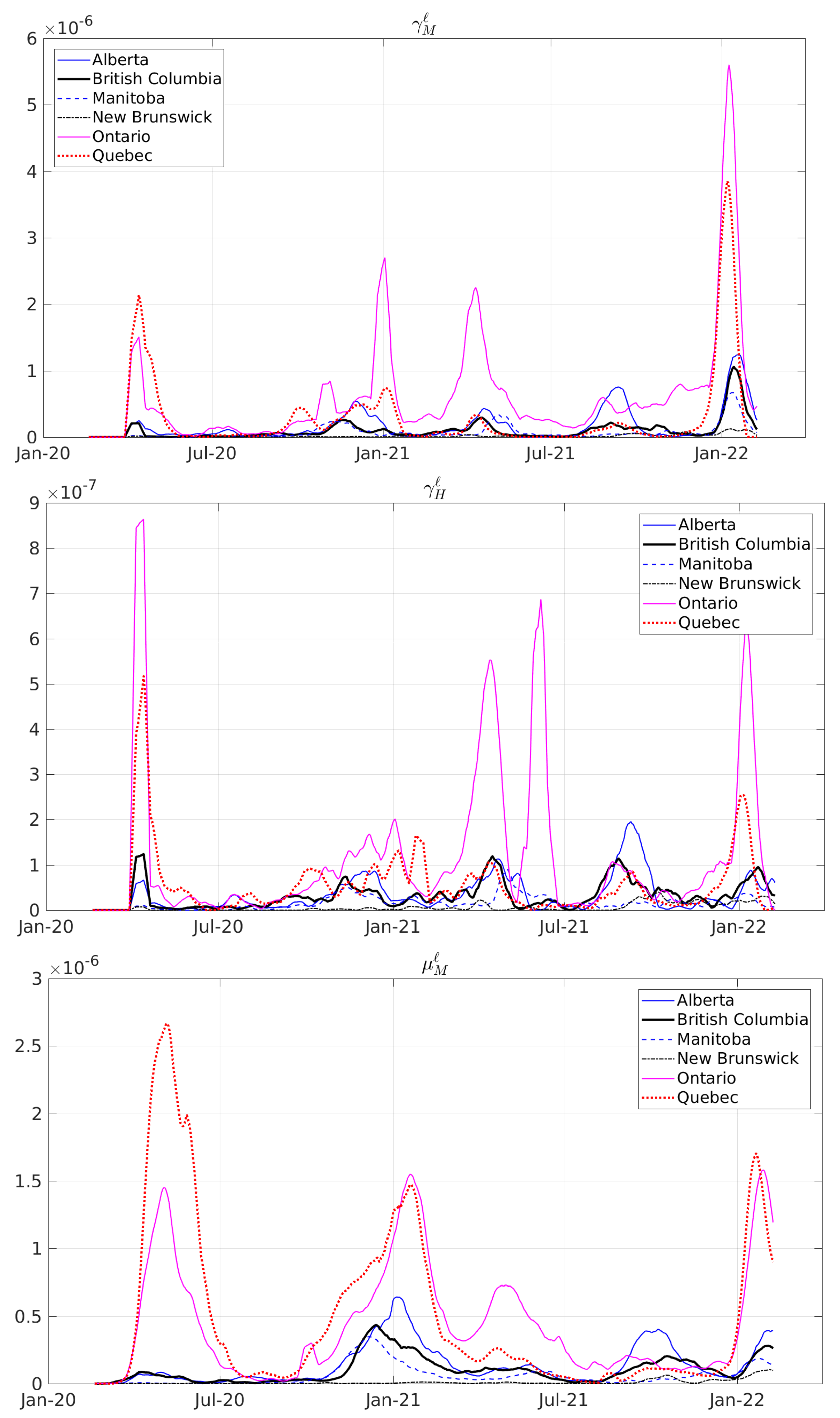
Figure 3.
Seven-day moving average of the time series for the estimated values of the baseline transition rates into employment and unemployment , as well as the sensitivities and of transition rates with respect to new infections for Alberta, British Columbia, Manitoba, New Brunswick, Ontario, and Quebec.
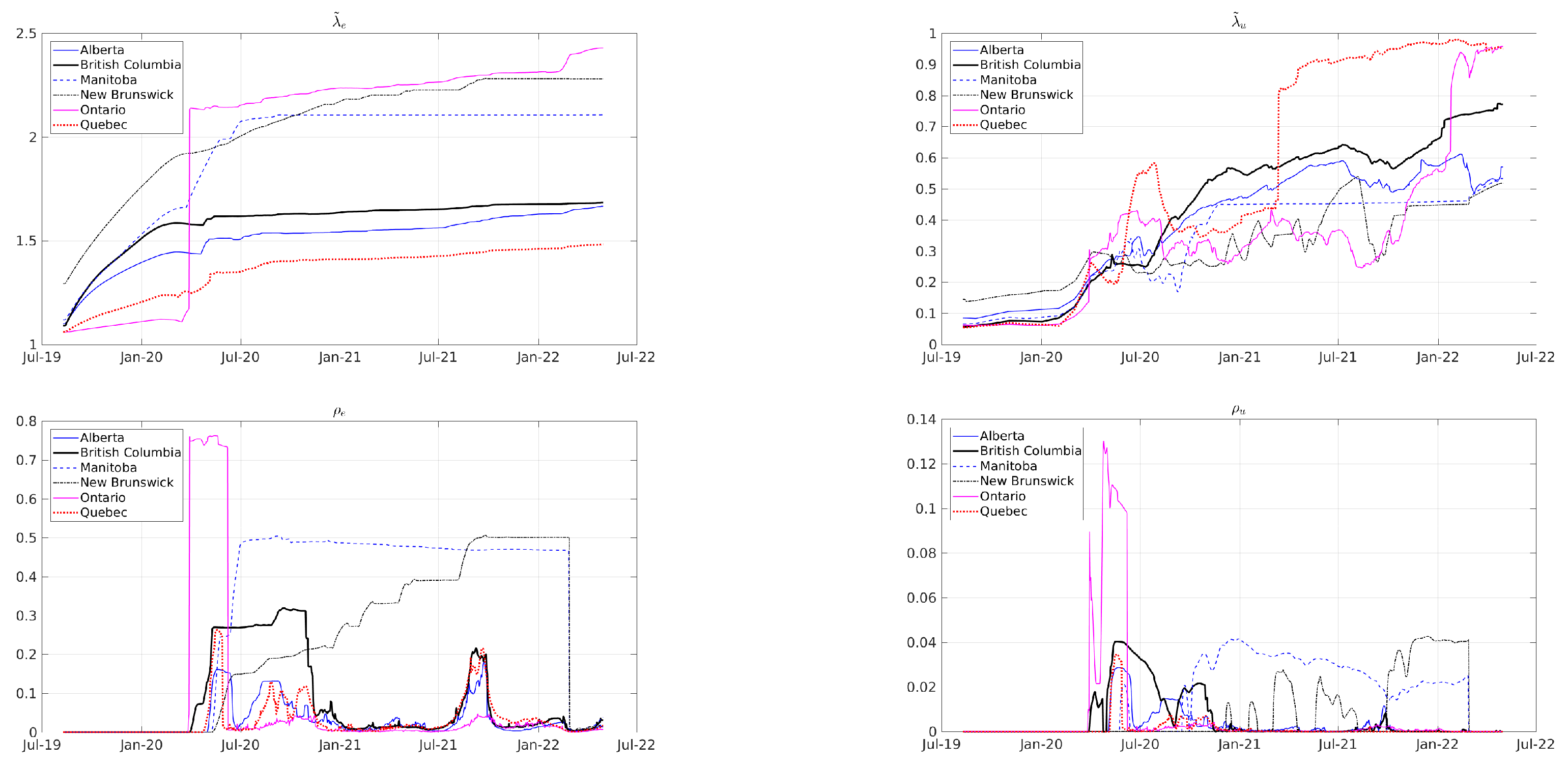
Figure 4.
Reported (blue area) seven-day moving average of daily COVID-19 infections, hospitalizations, ICU admissions, and deaths, as well as the monthly number of unemployed individuals, and their corresponding model predictions (solid lines) for Canada.
Figure 4.
Reported (blue area) seven-day moving average of daily COVID-19 infections, hospitalizations, ICU admissions, and deaths, as well as the monthly number of unemployed individuals, and their corresponding model predictions (solid lines) for Canada.
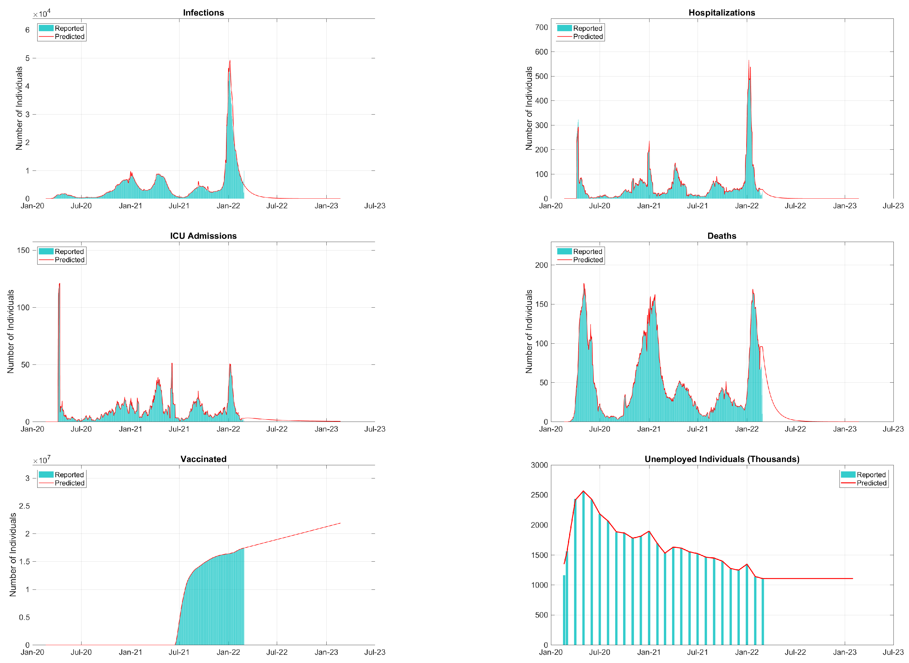
Figure 5.
Comparison between the 7-day moving average of daily reports (blue bars) of COVID-19 infections and the 30-day ahead model predictions (solid lines) for Canada. The dashed line separates the calibration dataset from the prediction/testing dataset.
Figure 5.
Comparison between the 7-day moving average of daily reports (blue bars) of COVID-19 infections and the 30-day ahead model predictions (solid lines) for Canada. The dashed line separates the calibration dataset from the prediction/testing dataset.
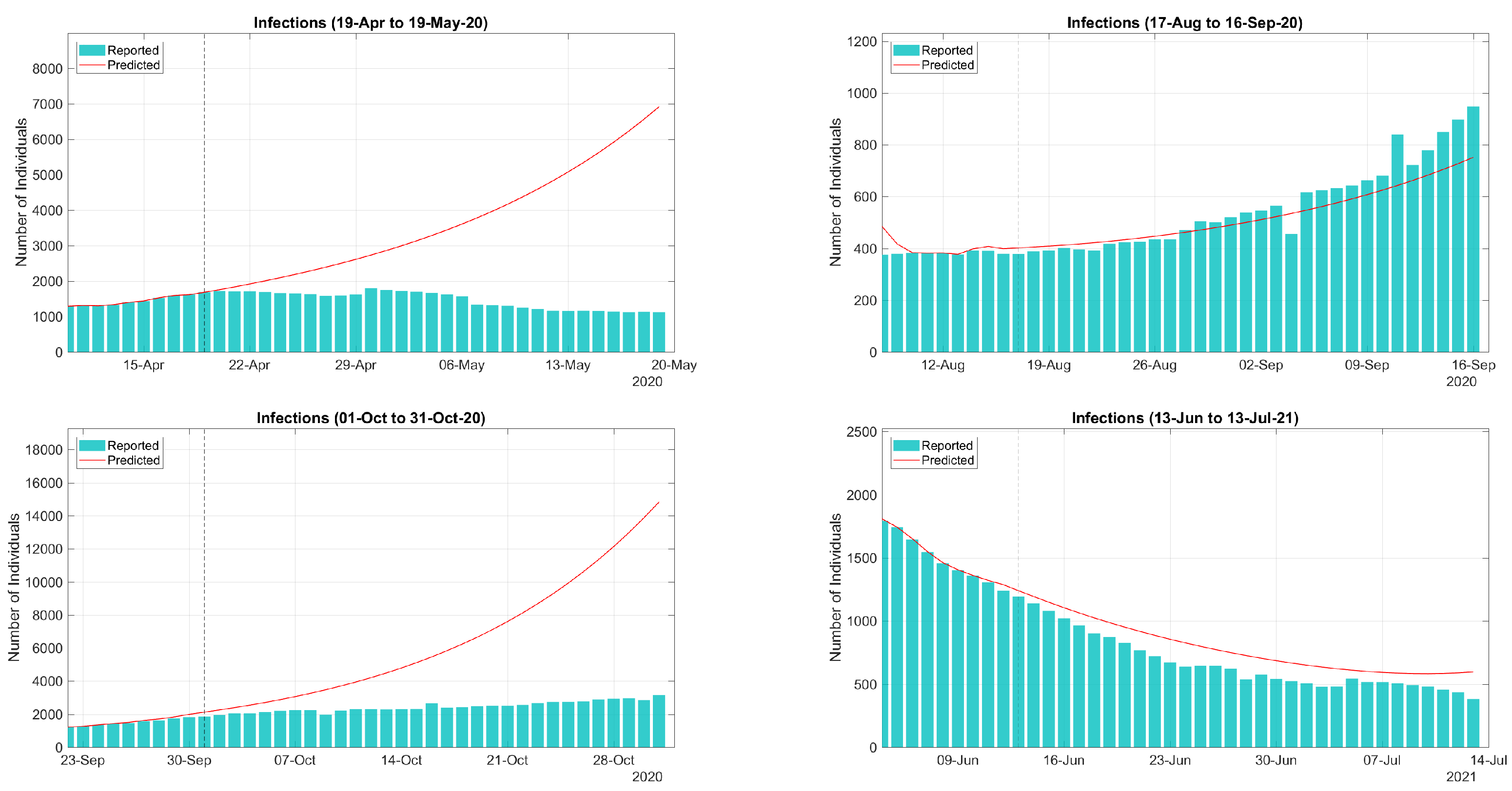
Figure 6.
Predictions of daily infections in Canada considering periodic vaccination booster campaigns with periods of 270, 360, 390, 450, 540, and 720 days.
Figure 6.
Predictions of daily infections in Canada considering periodic vaccination booster campaigns with periods of 270, 360, 390, 450, 540, and 720 days.

Figure 7.
Predictions of daily deaths in Canada considering periodic vaccination booster campaigns with periods of 270, 360, 390, 450, 540, and 720 days.
Figure 7.
Predictions of daily deaths in Canada considering periodic vaccination booster campaigns with periods of 270, 360, 390, 450, 540, and 720 days.

Figure 8.
Predictions of the daily number of unemployed individuals in Canada considering periodic vaccination booster campaigns with periods of 270, 360, 390, 450, 540, and 720 days.
Figure 8.
Predictions of the daily number of unemployed individuals in Canada considering periodic vaccination booster campaigns with periods of 270, 360, 390, 450, 540, and 720 days.
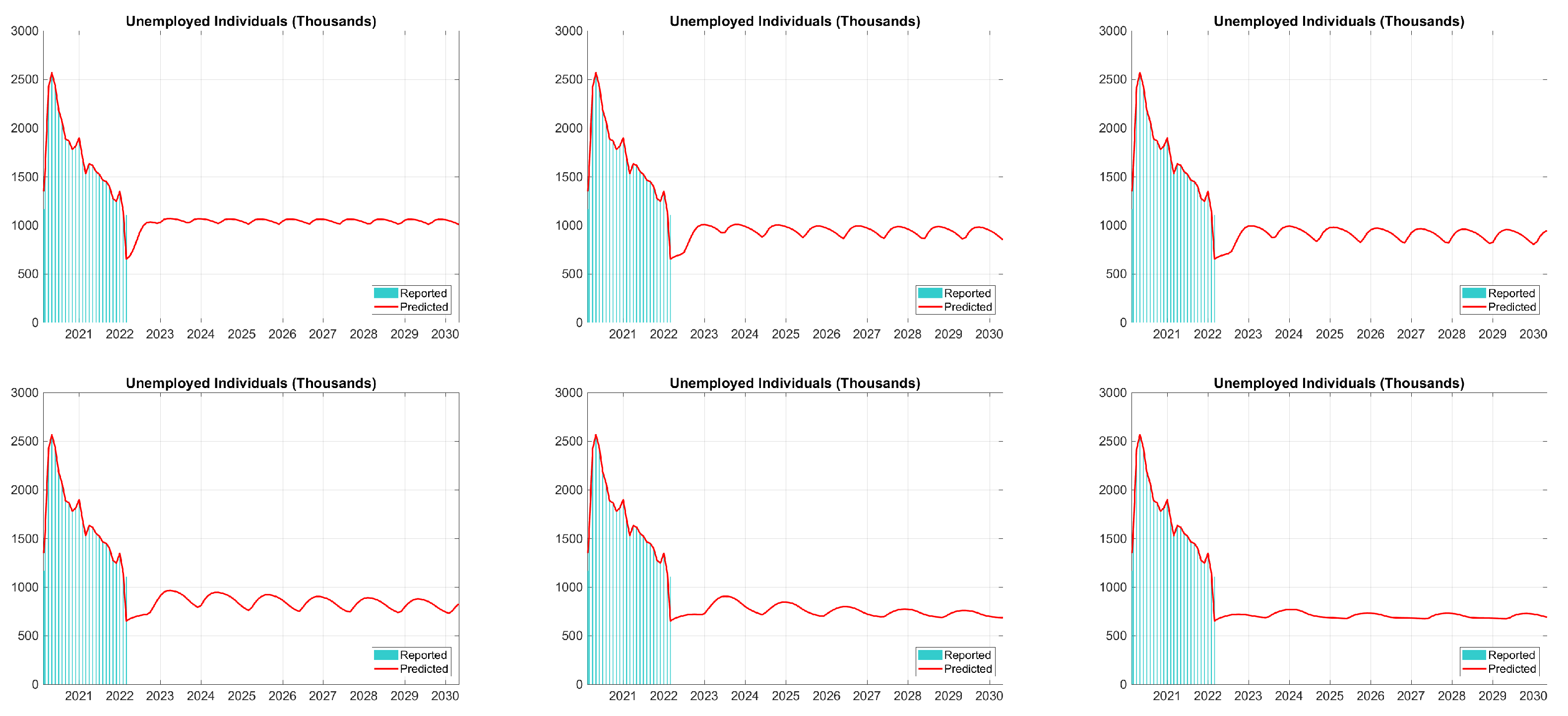
Figure 9.
Estimated values for k (top) and (bottom) in (34) by OLS method with 16-quarter running window.
Figure 9.
Estimated values for k (top) and (bottom) in (34) by OLS method with 16-quarter running window.
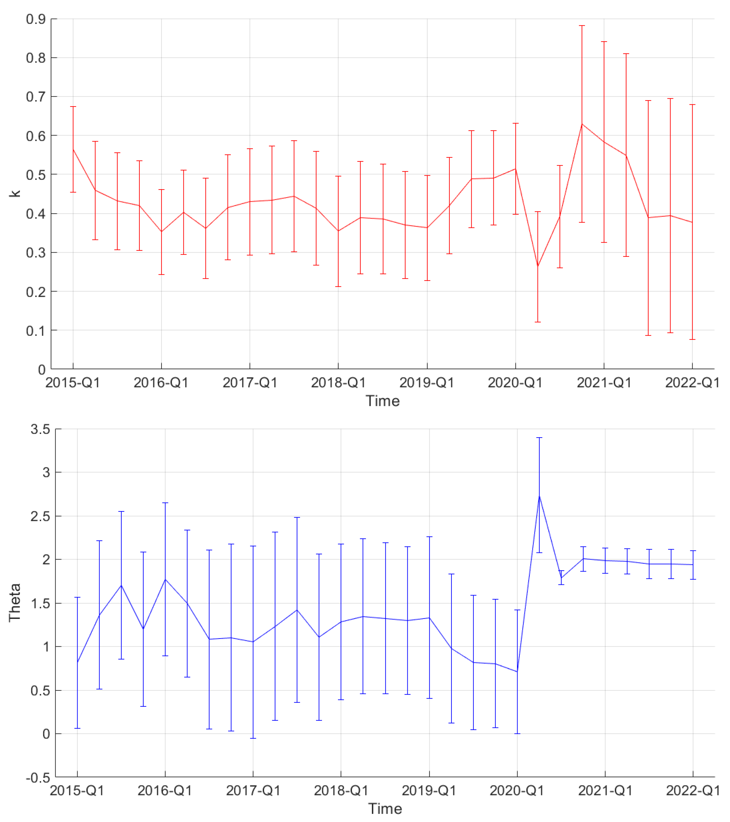
Figure 10.
Comparison between OECD and Stats Canada quarterly unemployment rates.
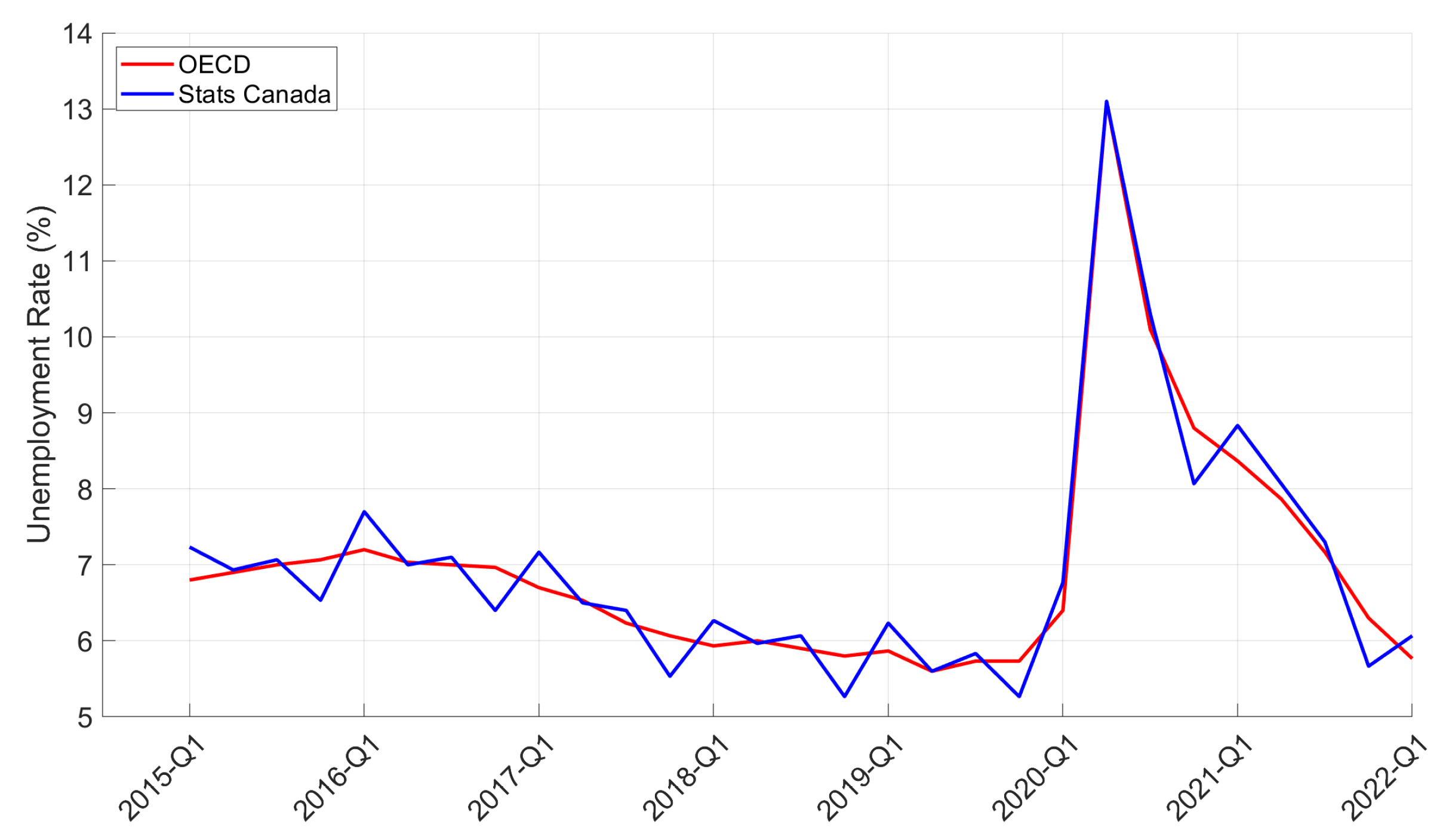
Figure 11.
Prediction of monthly unemployment rates considering periodic vaccination booster campaigns with periods of 270, 450, and 720 days.
Figure 11.
Prediction of monthly unemployment rates considering periodic vaccination booster campaigns with periods of 270, 450, and 720 days.

Figure 12.
Comparison between quarterly changes in GDP from OECD and Stats Canada data (top) and between OECD data and predictions based on Okun’s law (bottom).
Figure 12.
Comparison between quarterly changes in GDP from OECD and Stats Canada data (top) and between OECD data and predictions based on Okun’s law (bottom).
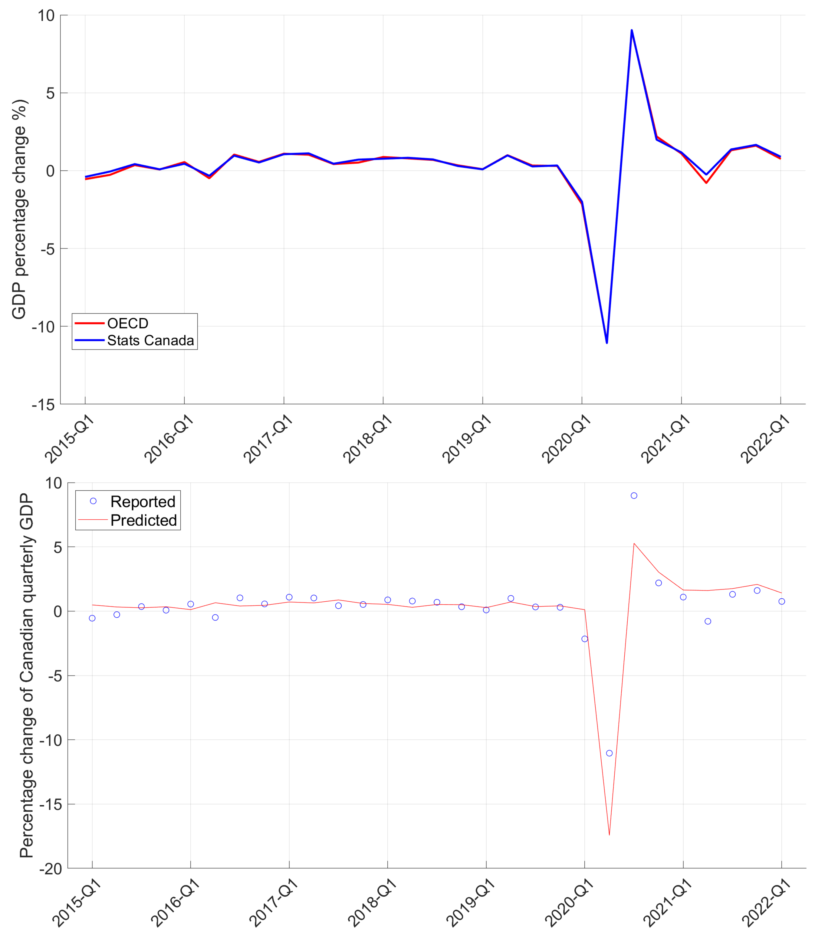
Figure 13.
Prediction of percentage change in quarterly GDP considering periodic vaccination booster campaigns with periods of 270, 450, and 720 days.
Figure 13.
Prediction of percentage change in quarterly GDP considering periodic vaccination booster campaigns with periods of 270, 450, and 720 days.

Table 1.
Out-of-sample model predictions (top rows) and observed (bottom rows) accumulated numbers of COVID-19 cases, hospitalizations, ICU admissions, and deaths in Canada. Predic. Error and Calib. Error stands for the out-of-sample prediction and calibration errors, respectively.
Table 1.
Out-of-sample model predictions (top rows) and observed (bottom rows) accumulated numbers of COVID-19 cases, hospitalizations, ICU admissions, and deaths in Canada. Predic. Error and Calib. Error stands for the out-of-sample prediction and calibration errors, respectively.
| Period | Cases | Hosp. | ICU Adm. | Deaths | Predic. Error | Calib. Error |
|---|---|---|---|---|---|---|
| 18 April to 24 April 2020 | 13,154 | 571 | 550 | 568 | 0.75% | 0.96% |
| 13,253 | 596 | 104 | 1084 | |||
| 28 May to 3 June 2020 | 6427 | 707 | 20 | 707 | 4.70% | 0.47% |
| 6744 | 33 | 30 | 868 | |||
| 17 June to 23 June 2020 | 2429 | 375 | 11 | 375 | 16.3% | 0.70% |
| 2902 | 36 | 12 | 304 | |||
| 27 July to 2 August 2020 | 3265 | 55 | 27 | 54 | 3.87% | 4.39% |
| 3397 | 63 | 26 | 57 | |||
| 5 September to 11 September 2020 | 4436 | 40 | 19 | 40 | 9.16% | 8.16% |
| 4883 | 57 | 19 | 28 | |||
| 15 October to 21 October 2020 | 18,846 | 166 | 50 | 166 | 2.89% | 1.50% |
| 19,407 | 238 | 71 | 172 | |||
| 24 November to 30 November 2020 | 38,963 | 494 | 107 | 494 | 13.4% | 6.02% |
| 45,013 | 548 | 100 | 655 | |||
| 3 January to 9 January 2021 | 84,386 | 841 | 83 | 840 | 29.8% | 13.85% |
| 65,000 | 1142 | 132 | 1140 | |||
| 12 February to 18 February 2021 | 22,904 | 700 | 43 | 700 | 2.25% | 1.90% |
| 23,431 | 131 | 43 | 525 | |||
| 24 March to 30 March 2021 | 32,367 | 214 | 88 | 213 | 12.82% | 0.82% |
| 37,127 | 417 | 141 | 230 | |||
| 3 May to 9 May 2021 | 55,040 | 350 | 175 | 349 | 9.03% | 1.43% |
| 60,503 | 477 | 73 | 372 | |||
| 12 June to 18 June 2021 | 8080 | 222 | 227 | 221 | 13.2% | 7.01% |
| 9304 | 104 | 110 | 185 | |||
| 2 July to 8 July 2021 | 3347 | 148 | 23 | 147 | 18.6% | 0.00% |
| 4110 | 108 | 12 | 123 | |||
| 20 September to 26 September 2021 | 31,751 | 197 | 135 | 196 | 7.53% | 1.24% |
| 34,335 | 482 | 117 | 287 | |||
| 30 October to 5 November 2021 | 15,023 | 243 | 38 | 243 | 16.8% | 1.11% |
| 18,065 | 240 | 34 | 227 | |||
| 19 November to 25 November 2021 | 18,165 | 177 | 40 | 176 | 13.7% | 0.32% |
| 21,037 | 300 | 48 | 170 | |||
| 9 December to 15 December 2021 | 28,110 | 137 | 59 | 137 | 19.1% | 0.57% |
| 34,767 | 324 | 69 | 162 | |||
| 29 December to 4 January 2021 | 443,096 | 122 | 70 | 122 | 56.4% | 9.83% |
| 283,268 | 1992 | 181 | 241 | |||
| 7 February to 13 February 2022 | 74,125 | 1044 | 58 | 1044 | 7.04% | 3.98% |
| 79,735 | 278 | 47 | 918 |
Table 2.
Estimated values, with standard deviations in brackets, of the parameters k and in (34) by the OLS method with a 16-quarter running window.
Table 2.
Estimated values, with standard deviations in brackets, of the parameters k and in (34) by the OLS method with a 16-quarter running window.
| Period | k | |
|---|---|---|
| 2019-Q4 | 0.49 (0.12) | 0.81 (0.74) |
| 2020-Q1 | 0.51 (0.12) | 0.71 (0.71) |
| 2020-Q2 | 0.26 (0.14) | 2.74 (0.66) |
| 2020-Q3 | 0.39 (0.13) | 1.79 (0.08) |
| 2020-Q4 | 0.63 (0.25) | 2.00 (0.14) |
| 2021-Q1 | 0.58 (0.26) | 1.98 (0.14) |
| 2021-Q2 | 0.55 (0.26) | 1.98 (0.14) |
| 2021-Q3 | 0.39 (0.30) | 1.95 (0.17) |
| 2021-Q4 | 0.39 (0.30) | 1.94 (0.17) |
| 2022-Q1 | 0.38 (0.30) | 1.94 (0.17) |
Publisher’s Note: MDPI stays neutral with regard to jurisdictional claims in published maps and institutional affiliations. |
© 2022 by the authors. Licensee MDPI, Basel, Switzerland. This article is an open access article distributed under the terms and conditions of the Creative Commons Attribution (CC BY) license (https://creativecommons.org/licenses/by/4.0/).
Share and Cite
MDPI and ACS Style
Albani, V.; Grasselli, M.; Pang, W.; Zubelli, J.P. The Interplay between COVID-19 and the Economy in Canada. J. Risk Financial Manag. 2022, 15, 476. https://doi.org/10.3390/jrfm15100476
AMA Style
Albani V, Grasselli M, Pang W, Zubelli JP. The Interplay between COVID-19 and the Economy in Canada. Journal of Risk and Financial Management. 2022; 15(10):476. https://doi.org/10.3390/jrfm15100476
Chicago/Turabian StyleAlbani, Vinicius, Matheus Grasselli, Weijie Pang, and Jorge P. Zubelli. 2022. "The Interplay between COVID-19 and the Economy in Canada" Journal of Risk and Financial Management 15, no. 10: 476. https://doi.org/10.3390/jrfm15100476