A General Family of Autoregressive Conditional Duration Models Applied to High-Frequency Financial Data

Abstract

In this paper, we propose a general family of Birnbaum–Saunders autoregressive conditional duration (BS-ACD) models based on generalized Birnbaum–Saunders (GBS) distributions, denoted by GBS-ACD. We further generalize these GBS-ACD models by using a Box-Cox transformation with a shape parameter $\lambda$ to the conditional median dynamics and an asymmetric response to shocks; this is denoted by GBS-AACD. We then carry out a Monte Carlo simulation study to evaluate the performance of the GBS-ACD models. Finally, an illustration of the proposed models is made by using New York stock exchange (NYSE) transaction data.

1. Introduction

The modeling of high-frequency financial data has been the focus of intense interest over the last decades. A prominent approach to modeling the durations between successive events (trades, quotes, price changes, etc.) was introduced by Engle and Russell (1998). These authors proposed the autoregressive conditional duration (ACD) model, which has some similarities with the ARCH (Engle 1982) and GARCH (Bollerslev 1986) models. The usefulness of appropriately modeling duration data is stressed by the relatively recent market microstructure literature; see Diamond and Verrechia (1987), Easley and O’Hara (1992), and Easley et al. (1997). Generalizations of the original ACD model are basically based on the following three aspects, i.e., (a) the distributional assumption in order to yield a unimodal failure rate (FR) (Grammig and Maurer 2000; Lunde 1999), (b) the linear form for the conditional mean (median) dynamics (Allen et al. 2008; Bauwens and Giot 2000; Fernandes and Grammig 2006), and (c) the time series properties (Bauwens and Giot 2003; Chiang 2007; De Luca and Zuccolotto 2006; Jasiak 1998; Zhang et al. 2001); see the reviews by Pacurar (2008) and Bhogal and Variyam Thekke (2019). Bhatti (2010) proposed a generalization of the ACD model that falls into all three branches above, based on the Birnbaum–Saunders (BS) distribution, denoted as the BS-ACD model. This model has several advantages over the traditional ACD ones; in particular, the BS-ACD model (1) has a realistic distributional assumption, that is, it provides both an asymmetric probability density function (PDF) and a unimodal FR shape; (2) it provides a natural parametrization of the point process in terms of a conditional median duration which is expected to improve the model fit despite a conditional mean duration, since the median is generally considered to be a better measure of central tendency than the mean for asymmetrical and heavy-tailed distributions; and (3) has easy implementation for estimation; see Ghosh and Mukherjee (2006), Bhatti (2010), Leiva et al. (2014), and Saulo et al. (2019).

Based on the relationship between the BS and symmetric distributions, Díaz-García and Leiva (2005) introduced generalized BS (GBS) distributions, obtaining a wider class of distributions that has either lighter or heavier tails than the BS density, allowing them to provide more flexibility. This new class essentially provides flexibility in the kurtosis level; see Sanhueza et al. (2008). In addition, the GBS distributions produce models whose parameter estimates are often robust to atypical data; see Leiva et al. (2008) and Barros et al. (2008). The GBS family includes as special cases the BS, BS-Laplace (BS-LA), BS-Logistic (BS-LO), BS-power-exponential (BS-PE), and BS-Student-t (BS-t) distributions.

The main aim of this work is to generalize the BS-ACD model, which was proposed by Bhatti (2010), based on GBS distributions (GBS-ACD). The proposed models should hold with the properties of the BS-ACD model, but, in addition, they should provide further properties and more flexibility. As mentioned before, the GBS family has models that have heavier tails than the BS density, and this characteristic is very useful in the modeling of high-frequency financial durations, since duration data are heavy-tailed and heavily right-skewed. We subsequently develop a class of augmented GBS-ACD (GBS-AACD) models by using the Box-Cox transformation (Box and Cox 1964) with a shape parameter $\lambda$$\ge 0$ to the conditional duration process and an asymmetric response to shocks; see Fernandes and Grammig (2006). Thus, the proposed GBS-ACD and GBS-AACD models would provide greater range and flexibility while fitting data. We apply the proposed models to high-frequency financial transaction (trade duration, TD) data. This type of data has unique features absent in data with low frequencies. For example, TD data (1) inherently arrive in irregular time intervals, (2) possess a large number of observations, (3) exhibit some diurnal pattern, i.e., activity is higher near the beginning and closing than in the middle of the trading day, and (4) present a unimodal failure rate; see Engle and Russell (1998) and Bhatti (2010). In addition, TD data have a relevant role in market microstructure theory, since they can be used as proxies for the existence of information in the market, and then serve as predictors for other market microstructure variables; see Mayorov (2011).

The rest of the paper proceeds as follows. Section 2 describes the BS and GBS distributions. In addition, some propositions are presented. Section 3 derives the GBS-ACD models associated with these distributions. Section 4 derives the GBS-AACD class of models. A Monte Carlo study of the proposed GBS-ACD model is performed in Section 5. Next, Section 6 presents an application of the proposed models to three data sets of New York stock exchange (NYSE) securities, and their fits are then assessed by a goodness-of-fit test. Finally, Section 7 offers some concluding remarks.

2. The Birnbaum–Saunders Distribution and Its Generalization

In this section, we describe the BS and GBS distributions and some of their properties.

The two-parameter BS distribution was introduced by Birnbaum and Saunders (1969) for modeling failure times of a material exposed to fatigue. They assumed that the fatigue failure follows from the development and growth of a dominant crack. Let $\mathit{\theta }={(\kappa ,\sigma )}^{\top }$ and

$$\begin{array}{c}\hfill a(x;\mathit{\theta })=\frac{1}{\kappa }\left[\sqrt{\frac{x}{\sigma }}-\sqrt{\frac{\sigma }{x}}\right],x>0\mathrm{and}\kappa ,\sigma >0.\end{array}$$

(1)

Expressions for the first, second, and third derivatives of the function $a(·;\mathit{\theta })$ are, respectively, given by

$$\begin{array}{c}{a}^{\prime }(x;\mathit{\theta })=\frac{1}{2\kappa \sigma }\left[{\left(\frac{\sigma }{x}\right)}^{1/2}+{\left(\frac{\sigma }{x}\right)}^{3/2}\right],a^{″}(x;\mathit{\theta })=-\frac{1}{4\kappa \sigma x}\left[{\left(\frac{\sigma }{x}\right)}^{1/2}+3{\left(\frac{\sigma }{x}\right)}^{3/2}\right],\\ a^{‴}(x;\mathit{\theta })=\frac{3}{8\kappa \sigma x^2}\left[{\left(\frac{\sigma }{x}\right)}^{1/2}+5{\left(\frac{\sigma }{x}\right)}^{3/2}\right].\end{array}$$

(2)

A random variable (RV) X has a BS distribution with parameter vector $\mathit{\theta }={(\kappa ,\sigma )}^{\top }$, denoted by $\mathrm{BS}\left(\mathit{\theta }\right)$, if it can be expressed as

$$\begin{array}{c}\hfill X=a^{-\mathbf{1}}(Z;\mathit{\theta })=\frac{\sigma }{4}{\left[\kappa Z+\sqrt{{\left(\kappa Z\right)}^2+4}\right]}^2,Z\sim N(0,1),\end{array}$$

(3)

where $a^{-\mathbf{1}}(·;\mathit{\theta })$ denotes the inverse function of $a(·;\mathit{\theta })$, $\kappa$ is a shape parameter, and when it decreases to zero, the BS distribution approaches the normal distribution with mean $\sigma$ and variance $\tau$, such that $\tau \to 0$ when $\kappa \to 0$. In addition, $\sigma$ is a scale parameter and also the median of the distribution $F_{\mathrm{BS}}\left(\sigma \right)=0.5$, where $F_{\mathrm{BS}}$ is the BS cumulative distribution function (CDF). The BS distribution holds proportionality and reciprocal properties given by $bX\sim BS(\kappa ,b\sigma )$, with $b>0$, and $1/X\sim BS(\kappa ,1/\sigma )$; see Saunders (1974). The probability density function (PDF) of a two-parameter BS random variable X is given by

$$\begin{array}{cc}\hfill f_{\mathrm{BS}}(x;\mathit{\theta })& =\varphi \left(a(x;\mathit{\theta })\right)a^{\prime }(x;\mathit{\theta }),x>0,\hfill \end{array}$$

(4)

where $\varphi (·)$ denotes the PDF of the standard normal distribution.

Díaz-García and Leiva (2005) proposed the GBS distribution by assuming that Z in (3) follows a symmetric distribution in $\mathbb{R}$, denoted by $X\sim GBS(\mathit{\theta },g)$, where g is a density generator function associated with the particular symmetric distribution. An RV Z has a standard symmetric distribution, denoted by $Z\sim \mathrm{S}(0,1;g)\equiv \mathrm{S}\left(g\right)$, if its density takes the form $f_Z\left(z\right)=cg\left(z^2\right)$ for $z\in \mathbb{R}$, where $g\left(u\right)$ with $u>0$ is a real function that generates the density of Z, and c is the normalization constant, that is, $c=1/{\int }_{-\infty }^{+\infty }g\left(z^2\right)dz$. Note that $U=Z^2\sim \mathrm{G}{\chi }^2(1;g)$, namely, U has a generalized chi-squared (G${\chi }^2$) distribution with one degree of freedom and density generator g; see Fang et al. (1990). Table 1 presents some characteristics and the values of $u_1\left(g\right)$, $u_2\left(g\right)$, $u_3\left(g\right)$, and $u_4\left(g\right)$ for the Laplace, logistic, normal, power-exponential (PE) and Student-t symmetric distributions, where $u_r\left(g\right)=\mathrm{E}\left[U^r\right]$ denotes the rth moment of U.

Table 1. Constants (c and $c_{g^2}$), density generators (g), and expressions of some moments $u_r\left(g\right)$ for the indicated distributions.

Dist.	c	$\mathit{g}=\mathit{g}\left(\mathit{u}\right)$, $\mathit{u}>0$	${\mathit{u}}_1\left(\mathit{g}\right)$	${\mathit{u}}_2\left(\mathit{g}\right)$	${\mathit{u}}_3\left(\mathit{g}\right)$	${\mathit{u}}_4\left(\mathit{g}\right)$
Laplace	$\frac{1}{2}$	$exp\left(-\left|u\right|\right)$	2!	4!	6!	8!
Logistic	1	$\frac{exp\left(u\right)}{{\left[1+exp\left(u\right)\right]}^2}$	$\approx 0.7957$	≈1.5097	≈4.2777	≈16.0142
Normal	$\frac{1}{\sqrt{2\pi }}$	$exp\left(-\frac{1}{2}u\right)$	1	3	15	105
PE	$\frac{\eta }{2^{\frac{1}{2\eta }}\Gamma \left(\frac{1}{2\eta }\right)}$	$exp\left(-\frac{1}{2}{u}^{\eta }\right),\eta >0$	$\frac{2^{\frac{1}{\eta }}\Gamma \left(\frac{3}{2\eta }\right)}{\Gamma \left(\frac{1}{2\eta }\right)}$	$\frac{2^{\frac{2}{\eta }}\Gamma \left(\frac{5}{2\eta }\right)}{\Gamma \left(\frac{1}{2\eta }\right)}$	$\frac{2^{\frac{3}{\eta }}\Gamma \left(\frac{7}{2\eta }\right)}{\Gamma \left(\frac{1}{2\eta }\right)}$	$\frac{2^{\frac{4}{\eta }}\Gamma \left(\frac{9}{2\eta }\right)}{\Gamma \left(\frac{1}{2\eta }\right)}$
t	$\frac{\Gamma \left(\frac{\eta +1}{2}\right)}{\sqrt{\eta \pi }\Gamma \left(\frac{\eta }{2}\right)}$	${\left(1+\frac{u}{\eta }\right)}^{-\frac{\eta +1}{2}},\eta >0$	$\frac{\eta }{(\eta -2)}$	$\frac{3{\eta }^2}{(\eta -2)(\eta -4)}$	$\frac{15{\eta }^3}{(\eta -2)(\eta -4)(\eta -6)}$	$\frac{105{\eta }^4}{(\eta -2)(\eta -4)(\eta -6)(\eta -8)}$
			$\eta >2$	$\eta >4$	$\eta >6$	$\eta >8$

Consider an RV Z such that $Z=a(X;\mathit{\theta })\sim S\left(g\right)$ so that

$$X=a^{-\mathbf{1}}(Z;\mathit{\theta })\sim GBS(\mathit{\theta },g).$$

(5)

The density associated with X in (5) is given by

$$\begin{array}{cc}\hfill f_{\mathrm{GBS}}(x;\mathit{\theta },g)& =cg\left(a^2(x;\mathit{\theta })\right)a^{\prime }(x;\mathit{\theta }),x>0,\hfill \end{array}$$

(6)

where, as mentioned earlier, g is the generator and c the normalizing constant associated with a particular symmetric density; see Table 1. The mean and variance of X are, respectively,

$$\begin{array}{c}\hfill \mathrm{E}\left[X\right]=\frac{\sigma }{2}(2+u_1{\kappa }^2),Var\left[X\right]=\frac{{\sigma }^2{\kappa }^2}{4}(2{\kappa }^2{u}_2+4u_1-{\kappa }^2{u}_1^2),\end{array}$$

(7)

where $u_r=u_r\left(g\right)=\mathrm{E}\left[U^r\right]$, with $U\sim \mathrm{G}{\chi }^2(1,g)$; see Table 1.

Based on Table 1, the expressions for the BS-LA, BS-LO, BS-PE, and BS-t densities are as follows:

$$\begin{array}{cc}\hfill f_{\mathrm{BS}-\mathrm{LA}}(x;\mathit{\theta })& =\frac{1}{4\kappa \sigma }exp\left(-\frac{1}{\kappa }\left|\sqrt{\frac{x}{\sigma }}-\sqrt{\frac{\sigma }{x}}\right|\right)\left[{\left(\frac{\sigma }{x}\right)}^{1/2}+{\left(\frac{\sigma }{x}\right)}^{3/2}\right],\hfill \\ \hfill f_{\mathrm{BS}-\mathrm{L}0}(x;\mathit{\theta })& =\frac{1}{2\kappa \sigma }\frac{exp\left(\frac{1}{\kappa }\left[\sqrt{\frac{x}{\sigma }}-\sqrt{\frac{\sigma }{x}}\right]\right)}{{\left[1+exp\left(\frac{1}{\kappa }\left[\sqrt{\frac{x}{\sigma }}-\sqrt{\frac{\sigma }{x}}\right]\right)\right]}^2}\left[{\left(\frac{\sigma }{x}\right)}^{1/2}+{\left(\frac{\sigma }{x}\right)}^{3/2}\right],\hfill \\ \hfill f_{\mathrm{BS}-\mathrm{PE}}(x;\mathit{\theta },\eta )& =\frac{\eta }{\Gamma \left(\frac{1}{2\eta }\right)2^{\frac{1}{2\eta }+1}\kappa \sigma }exp\left(-\frac{1}{2{\kappa }^{2\eta }}{\left[\frac{x}{\sigma }+\frac{\sigma }{x}-2\right]}^{\eta }\right)\left[{\left(\frac{\sigma }{x}\right)}^{1/2}+{\left(\frac{\sigma }{x}\right)}^{3/2}\right],\hfill \\ \hfill f_{\mathrm{BS}-t}(x;\mathit{\theta },\eta )& =\frac{\Gamma \left(\frac{\eta +1}{2}\right)}{2\sqrt{\eta \pi }\Gamma \left(\frac{\eta }{2}\right)\kappa \sigma }{\left[1+\frac{1}{\eta {\kappa }^2}\left(\frac{x}{\sigma }+\frac{\sigma }{x}-2\right)\right]}^{-\frac{\eta +1}{2}}\left[{\left(\frac{\sigma }{x}\right)}^{1/2}+{\left(\frac{\sigma }{x}\right)}^{3/2}\right],\hfill \\ \hfill & x>0\mathrm{and}\kappa ,\sigma ,\eta >0.\hfill \end{array}$$

Note that if $\eta =1$ (BS-PE) or if $\eta \to \infty$ (BS-t), then we obtain the BS distribution. It is worthwhile to point out that the BS-PE distribution has a greater (smaller) kurtosis than that of the BS distribution when $\eta <1$ ($\eta >1$). In addition, the BS-t distribution has a greater degree of kurtosis than that of the BS distribution for $\eta >8$; see Marchant et al. (2013).

Let

$$\begin{array}{c}\hfill b(h;\kappa ,\iota ,\varphi )=\frac{2}{\kappa }sinh\left(\frac{h-\iota }{\varphi }\right),h\in \mathbb{R},\kappa ,\varphi >0\mathrm{and}\iota \in \mathbb{R}.\end{array}$$

(8)

An alternative way to obtain GBS distributions is through sinh-symmetric (SHS) distributions. Díaz-García and Domínguez-Molina (2006) proposed SHS distributions by using the sinh-normal distribution introduced by Rieck and Nedelman (1991) in the symmetric case. They assumed the standard symmetrically distributed RV Z as follows:

$$Z=b(H;\kappa ,\iota ,\varphi )\sim \mathrm{S}\left(g\right).$$

(9)

Then,

$$H=b^{-\mathbf{1}}(Z;\kappa ,\iota ,\varphi )=\iota +\varphi arcsinh\left(\frac{\kappa Z}{2}\right)\sim SHS(\kappa ,\iota ,\varphi ,g).$$

(10)

The density associated with H in (10) is given by

$$\begin{array}{cc}\hfill f_{\mathrm{SHS}}(h;\kappa ,\iota ,\varphi ,g)& =cg\left(b^2(h;\kappa ,\iota ,\varphi )\right)b^{\prime }(h;\kappa ,\iota ,\varphi ),h\in \mathbb{R},\kappa ,\varphi >0\mathrm{and}\iota \in \mathbb{R},\hfill \end{array}$$

(11)

where g and c are as given in (6). A prominent result, which will be useful later on, is the following.

Proposition 1

(See Rieck and Nedelman (1991)). If $H\sim SHS(\kappa ,\iota =ln\sigma ,\varphi =2,g)$, then $X=exp\left(H\right)\sim GBS(\mathit{\theta },g)$, which is denoted by $H\sim log-GBS(\kappa ,\iota ,g)$.

3. The GBS-ACD Models

3.1. Existing ACD Models

Let $X_i=T_i-T_{i-1}$ denote the trade duration, i.e., the time elapsed between two transactions occurring at times $T_i$ and $T_{i-1}$. Engle and Russell (1998) assumed that the serial dependence commonly found in financial duration data is described by ${\psi }_i=\mathrm{E}\left[X_i\right|{\mathcal{F}}_{i-1}]$, where ${\psi }_i$ stands for the conditional mean of the ith trade duration based on the conditioning information set ${\mathcal{F}}_{i-1}$, which includes all information available at time $T_{i-1}$. The basic ACD($r,s$) model is then defined as

$$\begin{array}{ccc}\hfill X_i& =& {\psi }_i{\epsilon }_i,\hfill \\ \hfill {\psi }_i& =& \alpha +{\displaystyle \sum _{j=1}^r}{\beta }_j{\psi }_{i-j}+{\displaystyle \sum _{j=1}^s}{\gamma }_j{x}_{i-j},i=1,\dots ,n,\hfill \end{array}$$

(12)

where r and s refer to the orders of the lags and $\left\{{\epsilon }_i\right\}$ is an independent and identically distributed nonnegative sequence with PDF $f(·)$. Engle and Russell (1998) assumed a linear ACD(1,1) model defined by ${\psi }_i=\alpha +\beta x_{i-1}+\gamma {\psi }_{i-1}$, where $\alpha$, $\beta$, and $\gamma$ are the parameters. Note that a wide range of ACD model specifications may be defined by different distributions of ${\epsilon }_i$ and specifications of ${\psi }_i$; see Fernandes and Grammig (2006) and Pathmanathan et al. (2009).

An alternative ACD model is the Birnbaum–Saunders autoregressive conditional duration (BS-ACD) model proposed by Bhatti (2010). This approach takes into account the natural scale parameter in the $\mathrm{BS}\left(\mathit{\theta }\right)$ distribution to specify the BS-ACD model in terms of a time-varying conditional median duration ${\sigma }_i=F_{\mathrm{BS}}^{-1}(0.5|{\mathcal{F}}_{i-1})$, where $F_{\mathrm{BS}}$ denotes the CDF of the BS distribution. This specification has several advantages over the existing ACD models, as previously mentioned, including a realistic distributional assumption—an expected improvement in the model fit as a result of the natural parametrization in terms of the conditional median duration, since the median is generally considered to be a better measure of central tendency than the mean for asymmetrical and heavy-tailed distributions—and ease of fitting.

The PDF associated with the BS-ACD($r,s$) model is given by

$$f_{\mathrm{BS}}(x_i;{\mathbf{\theta }}_i)=\varphi \left(a(x_i;{\mathbf{\theta }}_i)\right)a^{\prime }(x_i;{\mathbf{\theta }}_i),i=1,\dots ,n,$$

(13)

where

$${\mathbf{\theta }}_i={(\kappa ,{\sigma }_i)}^{\top },i=1,\dots ,n,$$

with

$$ln{\sigma }_i=\alpha +{\sum }_{j=1}^r{\beta }_{j}ln{\sigma }_{i-j}+{\sum }_{j=1}^s{\gamma }_j\left[\frac{x_{i-j}}{{\sigma }_{i-j}}\right].$$

(14)

3.2. GBS-ACD Models

We now extend the class of BS-ACD($r,s$) models by using the GBS distributions. As explained earlier, this family of distributions possesses either lighter or heavier tails than the BS density, thus providing more flexibility. From the density given in (6), the GBS-ACD($r,s$) model can be obtained in a way analogous to that provided for the BS-ACD($r,s$) model in (13) with an associated PDF expressed as

$$f_{\mathrm{GBS}}(x_i;{\mathbf{\theta }}_i,g)=cg\left(a^2(x_i;{\mathbf{\theta }}_i)\right)a^{\prime }(x_i;{\mathbf{\theta }}_i),i=1,\dots ,n,$$

(15)

where c and g are as given in (6), ${\mathbf{\theta }}_i={(\kappa ,{\sigma }_i)}^{\top }$ for $i=1,\dots ,n$, with

$$ln{\sigma }_i=\alpha +{\sum }_{j=1}^r{\beta }_{j}ln{\sigma }_{i-j}+{\sum }_{j=1}^s{\gamma }_j\left[\frac{x_{i-j}}{{\sigma }_{i-j}}\right],$$

(16)

where $\mathbf{\xi }={(\kappa ,\alpha ,{\beta }_1,\dots ,{\beta }_r,{\gamma }_1,\dots ,{\gamma }_s)}^{\top }$ and $\mathbf{\zeta }={({\zeta }_1,\dots ,{\zeta }_k)}^{\top }$ denotes the additional parameters required by the density function in (6).

Note that model (15) can be written as

$$X_i={\sigma }_i{\phi }_i,$$

(17)

where ${\phi }_i=exp\left({\epsilon }_i\right)$ with ${\epsilon }_i$ being positively supported independent and identically distributed RVs following the $SHS(\kappa ,0,2,g)$ distribution, with density given by (11). Note that if ${\epsilon }_i\sim SHS(\kappa ,0,2,g)$, then $exp\left({\epsilon }_i\right)\sim GBS(\kappa ,1,g)$ (see Proposition 1) with $X_i\sim GBS({\mathbf{\theta }}_i,g)$.

3.2.1. Properties

Proposition 2 (Expected value of logarithmic duration in the GBS-ACD($r,s$) model).

Assuming that the process $\{X_i\sim \mathrm{GBS}({\mathbf{\theta }}_i,g):i=1,2,\dots \}$ is strictly stationary and that $\mathrm{E}\left[{\epsilon }_i\right]=\mu$, where ${\epsilon }_i$ is given in (17), we have

$$\mathrm{E}[ln{X}_i]=\frac{2[\alpha +\mu (1+{\sum }_{j=1}^r{\beta }_j)]+(2+u_1{\kappa }^2){\sum }_{j=1}^s{\gamma }_j}{2(1-{\sum }_{j=1}^r{\beta }_j)},\forall i,$$

whenever ${\sum }_{j=1}^r{\beta }_j\ne 1.$ The constant (depending only on the kernel g) $u_1$ is given in (7).

Proposition 3 (Moments of logarithmic duration in the GBS-ACD($1,1$) model).

If the process $\{X_i\sim \mathrm{GBS}({\mathbf{\theta }}_i,g):i=1,2,\dots \}$ is strictly stationary and $\mathrm{E}\left[{\epsilon }_i\right]=\mu$, where ${\epsilon }_i$ is given in (17), then

$$\begin{array}{c}\hfill \begin{array}{c}•\mathrm{E}[ln{X}_i]=\frac{2[\alpha +\mu (1+\beta )]+(2+u_1{\kappa }^2)\gamma }{2(1-\beta )},\beta \ne 1,\hfill \\ •\mathrm{E}\left[{(ln{X}_i)}^2\right]=\mu (2-\mu )+2\mu \mathrm{E}[ln{X}_i]+\hfill \\ \frac{{\alpha }^2-2\alpha \beta +\frac{{\gamma }^2}{2}(u_2{\kappa }^4+4u_1{\kappa }^2+2)+\gamma (2+u_1{\kappa }^2)(\alpha -\beta \mu )+[2\alpha \beta +\gamma \beta (2+u_1{\kappa }^2)]\mathrm{E}[ln{X}_i]}{1-{\beta }^2},\beta \ne \pm 1,\hfill \end{array},\forall i.\end{array}$$

3.2.2. Estimation

Let $(X_1,\dots ,X_n)$ be a sample from $X_i\sim \mathrm{GBS}({\mathbf{\theta }}_i,g)$ for $i=1,\dots ,n$, and let $\mathbf{x}={(x_1,\dots ,x_n)}^{\top }$ be the observed durations. Then, the log-likelihood function for $\mathbf{\xi }={(\kappa ,\alpha ,{\beta }_1,\dots ,{\beta }_r,{\gamma }_1,\dots ,{\gamma }_s)}^{\top }$ is obtained as

$$\begin{array}{c}\hfill {\ell }_{\mathrm{GBS}}\left(\mathbf{\xi }\right)={\displaystyle \sum _{i=1}^n}\left[ln\left(2c\right)-ln\kappa -ln{\sigma }_i+lng\left(a^2(x_i;{\mathit{\theta }}_i)\right)+ln\left({\left(\frac{{\sigma }_i}{x_i}\right)}^{1/2}+{\left(\frac{{\sigma }_i}{x_i}\right)}^{3/2}\right)\right],\end{array}$$

(18)

where the time-varying conditional median ${\sigma }_i$ is given as in (16). The maximum-likelihood (ML) estimates can be obtained by maximizing the expression defined in (18) by equating the score vector ${\dot{\ell }}_{\mathrm{GBS}}\left(\mathbf{\xi }\right)$, which contains the first derivatives of ${\ell }_{\mathrm{GBS}}\left(\mathbf{\xi }\right)$, to zero, providing the likelihood equations. They must be solved by an iterative procedure for non-linear optimization, such as the Broyden–Fletcher–Goldfarb–Shanno (BFGS) quasi-Newton method. It can easily be seen that the first-order partial derivatives of ${\ell }_{\mathrm{GBS}}\left(\mathbf{\xi }\right)$ are

$$\begin{array}{c}\hfill \frac{\partial {\ell }_{\mathrm{GBS}}}{\partial u}\left(\mathbf{\xi }\right)={\displaystyle \sum _{i=1}^n}\left[\frac{2a(x_i;{\mathbf{\theta }}_i)}{g\left(a^2(x_i;{\mathbf{\theta }}_i)\right)}\frac{\partial a(x_i;{\mathbf{\theta }}_i)}{\partial u}{g}^{\prime }\left(a^2(x_i;{\mathbf{\theta }}_i)\right)+\frac{1}{a^{\prime }(x_i;{\mathbf{\theta }}_i)}\frac{\partial a^{\prime }(x_i;{\mathbf{\theta }}_i)}{\partial u}\right],\end{array}$$

for each $u\in \{\kappa ,\alpha ,{\beta }_1,\dots ,{\beta }_r,{\gamma }_1,\dots ,{\gamma }_s\}$, where

$$\begin{array}{c}\hfill \begin{array}{ccc}\frac{\partial a(x_i;{\mathbf{\theta }}_i)}{\partial \kappa }=-\frac{a(x_i;{\mathbf{\theta }}_i)}{\kappa },\hfill & \hfill & \frac{\partial a(x_i;{\mathbf{\theta }}_i)}{\partial w}=\delta (x_i;{\mathbf{\theta }}_i)\frac{\partial {\sigma }_i}{\partial w}\hfill \\ \frac{\partial a^{\prime }(x_i;{\mathbf{\theta }}_i)}{\partial \kappa }=-\frac{a^{\prime }(x_i;{\mathbf{\theta }}_i)}{\kappa },\hfill & \hfill & \frac{\partial a^{\prime }(x_i;{\mathbf{\theta }}_i)}{\partial w}=\Delta (x_i;{\mathbf{\theta }}_i)\frac{\partial {\sigma }_i}{\partial w}\hfill \end{array},w\in \{\alpha ,{\beta }_1,\dots ,{\beta }_r,{\gamma }_1,\dots ,{\gamma }_s\},\end{array}$$

(19)

with $\delta (x_i;{\mathbf{\theta }}_i)=-\sqrt{x_i}{\left(2\kappa \sqrt{{\sigma }_i}\right)}^{-1}({\sigma }_i^{-1}-x_i^{-1})$ and $\Delta (x_i;{\mathbf{\theta }}_i)=-{\left(4\kappa \sqrt{x_i{\sigma }_i}\right)}^{-1}({\sigma }_i^{-1}+x_i^{-1}),$ and $i=1,\dots ,n.$ Here,

$$\begin{array}{c}\hfill \begin{array}{cc}\hfill & \frac{\partial {\sigma }_i}{\partial \alpha }=\left({\displaystyle {\sum }_{j=1}^r}\frac{{\beta }_j}{{\sigma }_{i-j}}\frac{\partial {\sigma }_{i-j}}{\partial \alpha }-{\displaystyle {\sum }_{j=1}^s}\frac{{\gamma }_j{x}_{i-j}}{{\sigma }_{i-j}^2}\frac{\partial {\sigma }_{i-j}}{\partial \alpha }\right){\sigma }_i,\hfill \\ \hfill & \frac{\partial {\sigma }_i}{\partial {\beta }_l}=\left({\beta }_{l}ln{\sigma }_{i-l}+{\displaystyle {\sum }_{j=1}^r}\frac{{\beta }_j}{{\sigma }_{i-j}}\frac{\partial {\sigma }_{i-j}}{\partial {\beta }_l}-{\displaystyle {\sum }_{j=1}^s}\frac{{\gamma }_j{x}_{i-j}}{{\sigma }_{i-j}^2}\frac{\partial {\sigma }_{i-j}}{\partial {\beta }_l}\right){\sigma }_i,l=1,\dots ,r,\hfill \\ \hfill & \frac{\partial {\sigma }_i}{\partial {\gamma }_m}=\left({\displaystyle {\sum }_{j=1}^r}\frac{{\beta }_j}{{\sigma }_{i-j}}\frac{\partial {\sigma }_{i-j}}{\partial {\gamma }_m}+{\gamma }_m\left[\frac{x_{i-m}}{{\sigma }_{i-m}}\right]-{\displaystyle {\sum }_{j=1}^s}\frac{{\gamma }_j{x}_{i-j}}{{\sigma }_{i-j}^2}\frac{\partial {\sigma }_{i-j}}{\partial {\gamma }_m}\right){\sigma }_i,m=1,\dots ,s.\hfill \end{array}\end{array}$$

(20)

The asymptotic distribution of the ML estimator $\widehat{\mathbf{\xi }}$ can be used to perform inference for $\mathbf{\xi }$. This estimator is consistent and has an asymptotic multivariate normal joint distribution with mean $\mathbf{\xi }$ and covariance matrix ${\Sigma }_{{}^{\widehat{\mathbf{\xi }}}}$, which may be obtained from the corresponding expected Fisher information matrix $\mathcal{I}\left(\mathbf{\xi }\right)$. Then,

$$\sqrt{n}[\widehat{\mathbf{\xi }}-\mathbf{\xi }]{\displaystyle \underset{}{\overset{\mathcal{D}}{\to }}}{\mathrm{N}}_{2+r+s}(\mathbf{0},{\Sigma }_{{}^{\widehat{\mathbf{\xi }}}}=\mathcal{J}{\left(\mathbf{\xi }\right)}^{-1}),$$

as $n\to \infty$, where ${\displaystyle \underset{}{\overset{\mathcal{D}}{\to }}}$ means “convergence in distribution” and $\mathcal{J}\left(\mathbf{\xi }\right)={lim}_{n\to \infty }[1/n]\mathcal{I}\left(\mathbf{\xi }\right)$. Notice that $\widehat{\mathcal{I}}{\left(\mathbf{\xi }\right)}^{-1}$ is a consistent estimator of the asymptotic variance–covariance matrix of $\widehat{\mathbf{\xi }}$. Here, we approximate the expected Fisher information matrix by its observed version obtained from the Hessian matrix ${\ddot{\ell }}_{\mathrm{GBS}}\left(\mathbf{\xi }\right)$, which contains the second derivatives of ${\ell }_{\mathrm{GBS}}\left(\mathbf{\xi }\right)$.

The elements of the Hessian are expressed as follows:

$$\begin{array}{cc}\frac{{\partial }^2{\ell }_{\mathrm{GBS}}}{\partial u\partial v}\left(\mathbf{\xi }\right)\hfill & ={\displaystyle \sum _{i=1}^n}[\frac{\partial \Theta (x_i;{\mathbf{\theta }}_i)}{\partial v}{g}^{\prime }\left(a^2(x_i;{\mathbf{\theta }}_i)\right)+2\Theta (x_i;{\mathbf{\theta }}_i)a(x_i;{\mathbf{\theta }}_i)\frac{\partial a(x_i;{\mathbf{\theta }}_i)}{\partial v}{g}^{″}\left(a^2(x_i;{\mathbf{\theta }}_i)\right)\hfill \\ \hfill & -\frac{1}{{\left(a^{\prime }(x_i;{\mathbf{\theta }}_i)\right)}^2}\frac{\partial a^{\prime }(x_i;{\mathbf{\theta }}_i)}{\partial u}\frac{\partial a^{\prime }(x_i;{\mathbf{\theta }}_i)}{\partial v}+\frac{1}{a^{\prime }(x_i;{\mathbf{\theta }}_i)}\frac{{\partial }^2{a}^{\prime }(x_i;{\mathbf{\theta }}_i)}{\partial u\partial v}],\hfill \end{array}$$

(21)

for each $u,v\in \{\kappa ,\alpha ,{\beta }_1,\dots ,{\beta }_r,{\gamma }_1,\dots ,{\gamma }_s\}$, where

$$\begin{array}{cc}\hfill & \Theta (x_i;{\mathbf{\theta }}_i)=\frac{2a(x_i;{\mathbf{\theta }}_i)}{g\left(a^2(x_i;{\mathbf{\theta }}_i)\right)}\frac{\partial a(x_i;{\mathbf{\theta }}_i)}{\partial u}\mathrm{and}\hfill \\ \hfill & \frac{\partial \Theta (x_i;{\mathbf{\theta }}_i)}{\partial v}=\frac{2}{g\left(a^2(x_i;{\mathbf{\theta }}_i)\right)}\left[\left(1-\frac{2a^2(x_i;{\mathbf{\theta }}_i)}{g\left(a^2(x_i;{\mathbf{\theta }}_i)\right)}\right)\frac{\partial a(x_i;{\mathbf{\theta }}_i)}{\partial u}\frac{\partial a(x_i;{\mathbf{\theta }}_i)}{\partial v}+a(x_i;{\mathbf{\theta }}_i)\frac{{\partial }^{2}a(x_i;{\mathbf{\theta }}_i)}{\partial u\partial v}\right].\hfill \end{array}$$

The partial derivatives $\frac{\partial a(x_i;{\mathbf{\theta }}_i)}{\partial u}$ and $\frac{\partial a^{\prime }(x_i;{\mathbf{\theta }}_i)}{\partial u}$ are given in (19). Furthermore, the second-order partial derivatives of $a(x_i;{\mathbf{\theta }}_i)$ and $a^{\prime }(x_i;{\mathbf{\theta }}_i)$ in (21), respectively, are given by

$$\begin{array}{c}\hfill \begin{array}{ccc}\frac{{\partial }^{2}a(x_i;{\mathbf{\theta }}_i)}{\partial {\kappa }^2}=\frac{2a(x_i;{\mathbf{\theta }}_i)}{{\kappa }^2},\hfill & \hfill & \frac{{\partial }^{2}a(x_i;{\mathbf{\theta }}_i)}{\partial w^2}=\frac{\sqrt{x_i}}{4\kappa {\sigma }_i^{3/2}}\left(\frac{1}{{\sigma }_i}-\frac{1}{x_i}\right){\left(\frac{\partial {\sigma }_i}{\partial w}\right)}^2+\delta (x_i;{\mathbf{\theta }}_i)\frac{{\partial }^2{\sigma }_i}{\partial w^2},\hfill \\ \frac{{\partial }^2{a}^{\prime }(x_i;{\mathbf{\theta }}_i)}{\partial {\kappa }^2}=\frac{2a^{\prime }(x_i;{\mathbf{\theta }}_i)}{{\kappa }^2},\hfill & \hfill & \frac{{\partial }^2{a}^{\prime }(x_i;{\mathbf{\theta }}_i)}{\partial w^2}=\frac{2\kappa }{\sqrt{x_i}{\sigma }_i^{3/2}}\left(\frac{1}{{\sigma }_i}+\frac{1}{x_i}\right){\left(\frac{\partial {\sigma }_i}{\partial w}\right)}^2+\Delta (x_i;{\mathbf{\theta }}_i)\frac{{\partial }^2{\sigma }_i}{\partial w^2},\hfill \end{array}\end{array}$$

for each $w\in \{\alpha ,{\beta }_1,\dots ,{\beta }_r,{\gamma }_1,\dots ,{\gamma }_s\}$, with $\delta (x_i;{\mathbf{\theta }}_i)=-\sqrt{x_i}{\left(2\kappa \sqrt{{\sigma }_i}\right)}^{-1}({\sigma }_i^{-1}-x_i^{-1})$ and $\Delta (x_i;{\mathbf{\theta }}_i)=-{\left(4\kappa \sqrt{x_i{\sigma }_i}\right)}^{-1}({\sigma }_i^{-1}+x_i^{-1}).$ Here,

$$\begin{array}{c}\hfill \begin{array}{cc}\hfill & \frac{{\partial }^2{\sigma }_i}{\partial {\alpha }^2}=\left[-{\displaystyle \sum _{j=1}^r}\frac{{\beta }_j}{{\sigma }_{i-j}}\left(\frac{1}{{\sigma }_{i-j}}{\left(\frac{\partial {\sigma }_{i-j}}{\partial \alpha }\right)}^2-\frac{{\partial }^2{\sigma }_{i-j}}{\partial {\alpha }^2}\right)+{\displaystyle \sum _{j=1}^s}\frac{{\gamma }_j{x}_{i-j}}{{\sigma }_{i-j}^2}\left(\frac{2}{{\sigma }_{i-j}}{\left(\frac{\partial {\sigma }_{i-j}}{\partial \alpha }\right)}^2-\frac{{\partial }^2{\sigma }_{i-j}}{\partial {\alpha }^2}\right)\right]{\sigma }_i+\frac{1}{{\sigma }_i}{\left(\frac{\partial {\sigma }_i}{\partial \alpha }\right)}^2,\hfill \\ \hfill & \frac{{\partial }^2{\sigma }_i}{\partial {\beta }_l^2}=\left[ln{\sigma }_{i-l}+\frac{{\beta }_l}{{\sigma }_{i-l}}\frac{\partial {\sigma }_{i-l}}{\partial {\beta }_l}-{\displaystyle \sum _{j=1}^r}\frac{{\beta }_j}{{\sigma }_{i-j}}\left(\frac{1}{{\sigma }_{i-j}}{\left(\frac{\partial {\sigma }_{i-j}}{\partial {\beta }_l}\right)}^2-\frac{{\partial }^2{\sigma }_{i-j}}{\partial {\beta }_l^2}\right)+{\displaystyle \sum _{j=1}^s}\frac{{\gamma }_j{x}_{i-j}}{{\sigma }_{i-j}^2}\left(\frac{2}{{\sigma }_{i-j}}{\left(\frac{\partial {\sigma }_{i-j}}{\partial {\beta }_l}\right)}^2-\frac{{\partial }^2{\sigma }_{i-j}}{\partial {\beta }_l^2}\right)\right]{\sigma }_i\hfill \\ \hfill & +\frac{1}{{\sigma }_i}{\left(\frac{\partial {\sigma }_i}{\partial {\beta }_l}\right)}^2,l=1,\dots ,r,\hfill \\ \hfill & \frac{{\partial }^2{\sigma }_i}{\partial {\gamma }_m^2}=\left[-{\displaystyle \sum _{j=1}^r}\frac{{\beta }_j}{{\sigma }_{i-j}}\left(\frac{1}{{\sigma }_{i-j}}{\left(\frac{\partial {\sigma }_{i-j}}{\partial {\gamma }_m}\right)}^2-\frac{{\partial }^2{\sigma }_{i-j}}{\partial {\gamma }_m^2}\right)+\frac{x_{i-m}}{{\sigma }_{i-m}}-\frac{x_{i-m}}{{\sigma }_{i-m}^2}\frac{\partial {\sigma }_{i-m}}{\partial {\gamma }_m}+{\displaystyle \sum _{j=1}^s}\frac{{\gamma }_j{x}_{i-j}}{{\sigma }_{i-j}^2}\left(\frac{2}{{\sigma }_{i-j}}{\left(\frac{\partial {\sigma }_{i-j}}{\partial {\gamma }_m}\right)}^2-\frac{{\partial }^2{\sigma }_{i-j}}{\partial {\gamma }_m^2}\right)\right]{\sigma }_i\hfill \\ \hfill & +\frac{1}{{\sigma }_i}{\left(\frac{\partial {\sigma }_i}{\partial {\gamma }_m}\right)}^2,m=1,\dots ,s;i=1,\dots ,n.\hfill \end{array}\end{array}$$

Note that the functions $a(x_i;{\mathbf{\theta }}_i)$ and $a^{\prime }(x_i;{\mathbf{\theta }}_i)$ have continuous second-order partial derivatives at a given point ${\mathbf{\theta }}_i\in {\mathbb{R}}^4$, $i=1,\dots ,n$. Then, by Schwarz’s Theorem, it follows that the partial differentiations of these functions are commutative at that point, that is, $\frac{{\partial }^{2}a(x_i;{\mathbf{\theta }}_i)}{\partial u\partial v}=\frac{{\partial }^{2}a(x_i;{\mathbf{\theta }}_i)}{\partial v\partial u}$ and $\frac{{\partial }^2{a}^{\prime }(x_i;{\mathbf{\theta }}_i)}{\partial u\partial v}=\frac{{\partial }^2{a}^{\prime }(x_i;{\mathbf{\theta }}_i)}{\partial v\partial u},$ for each $u\ne v\in \{\kappa ,\alpha ,{\beta }_1,\dots ,{\beta }_r,{\gamma }_1,\dots ,{\gamma }_s\}.$ With this in mind, the mixed partial derivatives of $a(x_i;{\mathbf{\theta }}_i)$ and $a^{\prime }(x_i;{\mathbf{\theta }}_i)$ in (21) have the following form:

$$\begin{array}{c}\hfill \begin{array}{c}\frac{{\partial }^{2}a(x_i;{\mathbf{\theta }}_i)}{\partial \kappa \partial w_1}=-\frac{1}{\kappa }\frac{\partial a(x_i;{\mathbf{\theta }}_i)}{\partial w_1},\hfill \\ \frac{{\partial }^{2}a(x_i;{\mathbf{\theta }}_i)}{\partial \alpha \partial w_2}=\frac{\sqrt{x_i}}{4\kappa {\sigma }_i^{3/2}}\left(\frac{1}{{\sigma }_i}-\frac{1}{x_i}\right)\frac{\partial {\sigma }_i}{\partial \alpha }\frac{\partial {\sigma }_i}{\partial w_2}+\delta (x_i;{\mathbf{\theta }}_i)\frac{{\partial }^2{\sigma }_i}{\partial \alpha \partial w_2},\hfill \\ \frac{{\partial }^{2}a(x_i;{\mathbf{\theta }}_i)}{\partial {\beta }_l\partial {\gamma }_m}=\frac{\sqrt{x_i}}{4\kappa {\sigma }_i^{3/2}}\left(\frac{1}{{\sigma }_i}-\frac{1}{x_i}\right)\frac{\partial {\sigma }_i}{\partial {\beta }_l}\frac{\partial {\sigma }_i}{\partial {\gamma }_m}+\delta (x_i;{\mathbf{\theta }}_i)\frac{{\partial }^2{\sigma }_i}{\partial {\beta }_l\partial {\gamma }_m},\hfill \\ \frac{{\partial }^2{a}^{\prime }(x_i;{\mathbf{\theta }}_i)}{\partial \kappa \partial w_1}=-\frac{1}{\kappa }\frac{\partial a^{\prime }(x_i;{\mathbf{\theta }}_i)}{\partial w_1},\hfill \\ \frac{{\partial }^2{a}^{\prime }(x_i;{\mathbf{\theta }}_i)}{\partial \alpha \partial w_2}=\frac{2\kappa }{\sqrt{x_i}{\sigma }_i^{3/2}}\left(\frac{1}{{\sigma }_i}+\frac{1}{x_i}\right)\frac{\partial {\sigma }_i}{\partial \alpha }\frac{\partial {\sigma }_i}{\partial w_2}+\Delta (x_i;{\mathbf{\theta }}_i)\frac{{\partial }^2{\sigma }_i}{\partial \alpha \partial w_2},\hfill \\ \frac{{\partial }^2{a}^{\prime }(x_i;{\mathbf{\theta }}_i)}{\partial {\beta }_l\partial {\gamma }_m}=\frac{2\kappa }{\sqrt{x_i}{\sigma }_i^{3/2}}\left(\frac{1}{{\sigma }_i}+\frac{1}{x_i}\right)\frac{\partial {\sigma }_i}{\partial {\beta }_l}\frac{\partial {\sigma }_i}{\partial {\gamma }_m}+\Delta (x_i;{\mathbf{\theta }}_i)\frac{{\partial }^2{\sigma }_i}{\partial {\beta }_l\partial {\gamma }_m},\hfill \end{array}\end{array}$$

for each $w_1\in \{\alpha ,{\beta }_1,\dots ,{\beta }_r,{\gamma }_1,\dots ,{\gamma }_s\}$, $w_2\in \{{\beta }_1,\dots ,{\beta }_r,{\gamma }_1,\dots ,{\gamma }_s\}$, and $l=1,\dots ,r$; $m=1,\dots ,s$, where $\delta (x_i;{\mathbf{\theta }}_i)$ and $\Delta (x_i;{\mathbf{\theta }}_i)$ are as before. In the above identities, the mixed partial derivatives $\frac{{\partial }^2{\sigma }_i}{\partial \alpha \partial w_2}$ and $\frac{{\partial }^2{\sigma }_i}{\partial {\beta }_l\partial {\gamma }_m}$, respectively, are given by

$$\begin{array}{c}\frac{{\partial }^2{\sigma }_i}{\partial \alpha \partial w_2}=\left[-{\displaystyle {\sum }_{j=1}^r}\frac{{\beta }_j}{{\sigma }_{i-j}}\left(\frac{1}{{\sigma }_{i-j}}\frac{\partial {\sigma }_{i-j}}{\partial \alpha }\frac{\partial {\sigma }_{i-j}}{\partial w_2}-\frac{{\partial }^2{\sigma }_{i-j}}{\partial \alpha \partial w_2}\right)+{\displaystyle {\sum }_{j=1}^s}\frac{{\gamma }_j{x}_{i-j}}{{\sigma }_{i-j}^2}\left(\frac{2}{{\sigma }_{i-j}}\frac{\partial {\sigma }_{i-j}}{\partial \alpha }\frac{\partial {\sigma }_{i-j}}{\partial w_2}-\frac{{\partial }^2{\sigma }_{i-j}}{\partial \alpha \partial w_2}\right)\right]{\sigma }_i+\frac{1}{{\sigma }_i}\frac{\partial {\sigma }_i}{\partial \alpha }\frac{\partial {\sigma }_i}{\partial w_2},\hfill \\ \frac{{\partial }^2{\sigma }_i}{\partial {\beta }_l\partial {\gamma }_m}=\left[\frac{{\beta }_l}{{\sigma }_{i-l}}\frac{\partial {\sigma }_{i-l}}{\partial {\gamma }_m}-{\displaystyle {\sum }_{j=1}^r}\frac{{\beta }_j}{{\sigma }_{i-j}}\left(\frac{1}{{\sigma }_{i-j}}\frac{\partial {\sigma }_{i-j}}{\partial {\beta }_l}\frac{\partial {\sigma }_{i-j}}{\partial {\gamma }_m}-\frac{{\partial }^2{\sigma }_{i-j}}{\partial {\beta }_l\partial {\gamma }_m}\right)+{\displaystyle {\sum }_{j=1}^s}\frac{{\gamma }_j{x}_{i-j}}{{\sigma }_{i-j}^2}\left(\frac{2}{{\sigma }_{i-j}}\frac{\partial {\sigma }_{i-j}}{\partial {\beta }_l}\frac{\partial {\sigma }_{i-j}}{\partial {\gamma }_m}-\frac{{\partial }^2{\sigma }_{i-j}}{\partial {\beta }_l\partial {\gamma }_m}\right)\right]{\sigma }_i\hfill \\ +\frac{1}{{\sigma }_i}\frac{\partial {\sigma }_i}{\partial {\beta }_l}\frac{\partial {\sigma }_i}{\partial {\gamma }_m},l=1,\dots ,r;m=1,\dots ,s\mathrm{and}i=1,\dots ,n.\hfill \end{array}$$

3.2.3. Residual Analysis

We carry out goodness-of-fit through residual analysis. In particular, we consider the generalized Cox–Snell residual, which is given by

$$r^{\mathrm{cs}}=-ln\widehat{S}\left(x_i\right|{\mathcal{F}}_{i-1}),$$

(22)

where $\widehat{S}\left(x_i\right|{\mathcal{F}}_{i-1})$ denotes the fitted conditional survival function. When the model is correctly specified, the Cox–Snell residual has a unit exponential ($EXP\left(1\right)$) distribution; see Bhatti (2010).

4. The GBS-AACD Models

Now, we introduce a generalization of the linear form for the conditional median dynamics based on the Box-Cox transformation; see Box and Cox (1964) and Fernandes and Grammig (2006) for pertinent details. Hereafter, we use the log-linear form ${\sigma }_i$ given in (16) with $r=1$ and $s=1$ (i.e., the GBS-ACD($r=1,s=1$) model, which we abbreviate as the GBS-ACD model, since a higher-order model does not increase the distributional fit of the residuals (Bhatti 2010)). Therefore, (16) results in

$$ln{\sigma }_i=\alpha +\beta ln{\sigma }_{i-1}+\gamma \left[\frac{x_{i-1}}{{\sigma }_{i-1}}\right].$$

(23)

The asymmetric version of the GBS-ACD model—GBS-AACD model—is given by

$${\sigma }_i=\alpha +\beta {\sigma }_{i-1}+\gamma {\sigma }_{i-1}\left(|{\phi }_{i-1}-b|+c({\phi }_{i-1}-b)\right),$$

(24)

where b and c are the shift and rotation parameters, respectively. By applying the Box-Cox transformation with parameter $\lambda \ge 0$ to the conditional duration model process ${\sigma }_i$ and introducing the parameter $\nu$, we can write (24) as

$$\frac{{\sigma }_i^{\lambda }-1}{\lambda }={\alpha }_{*}+\beta \frac{{\sigma }_{i-1}^{\lambda }-1}{\lambda }+{\gamma }_{*}{\sigma }_{i-1}^{\lambda }{\left(|{\phi }_{i-1}-b|+c({\phi }_{i-1}-b)\right)}^{\nu }.$$

(25)

The parameter $\lambda$ determines the shape of the transformation, i.e., concave ($\lambda \le 1$) or convex ($\lambda \ge 1$), and the parameter $\nu$ aims to transform the (potentially shifted and rotated) term $\left(|{\phi }_{i-1}-b|+c({\phi }_{i-1}-b)\right)$. Setting $\alpha =\lambda {\alpha }_{*}-\beta +1$ and $\gamma =\lambda {\gamma }_{*}$, we obtain

$${\sigma }_i^{\lambda }=\alpha +\beta {\sigma }_{i-1}^{\lambda }+\gamma {\sigma }_{i-1}^{\lambda }{\left(|{\phi }_{i-1}-b|+c({\phi }_{i-1}-b)\right)}^{\nu }.$$

(26)

We present below the forms of GBS-AACD models obtained from different specifications. Note that the Logarithmic GBS-ACD type II is equivalent to (23).

• Augmented ACD (GBS-AACD):

  $${\sigma }_i^{\lambda }=\alpha +\beta {\sigma }_{i-1}^{\lambda }+\gamma {\sigma }_{i-1}^{\lambda }{\left(|{\phi }_{i-1}-b|+c({\phi }_{i-1}-b)\right)}^{\nu }.$$
• Asymmetric power ACD (GBS-A-PACD) ($\lambda =\nu$):

  $${\sigma }_i^{\lambda }=\alpha +\beta {\sigma }_{i-1}^{\lambda }+\gamma {\sigma }_{i-1}^{\lambda }{\left(|{\phi }_{i-1}-b|+c({\phi }_{i-1}-b)\right)}^{\lambda }.$$
• Asymmetric logarithmic ACD (GBS-A-LACD) ($\lambda \to 0$ and $\nu =1$):

  $$ln{\sigma }_i=\alpha +\beta ln{\sigma }_{i-1}+\gamma \left(|{\phi }_{i-1}-b|+c({\phi }_{i-1}-b)\right).$$
• Asymmetric ACD (GBS-A-ACD) ($\lambda =\nu =1$):

  $${\sigma }_i=\alpha +\beta {\sigma }_{i-1}+\gamma {\sigma }_{i-1}\left(|{\phi }_{i-1}-b|+c({\phi }_{i-1}-b)\right).$$
• Power ACD (GBS-PACD) ($\lambda =\nu$ and $b=c=0$):

  $${\sigma }_i^{\lambda }=\alpha +\beta {\sigma }_{i-1}^{\lambda }+\gamma x_{i-1}^{\lambda }.$$
• Box-Cox ACD (GBS-BCACD) ($\lambda \to 0$ and $b=c=0$):

  $$ln{\sigma }_i=\alpha +\beta ln{\sigma }_{i-1}+\gamma {\phi }_{i-1}^{\nu }.$$
• Logarithmic ACD type I (GBS-LACD I) ($\lambda ,\nu \to 0$ and $b=c=0$):

  $$ln{\sigma }_i=\alpha +\beta ln{\sigma }_{i-1}+\gamma ln{x}_{i-1}.$$
• Logarithmic ACD type II (GBS-LACD II) ($\lambda \to 0$, $\nu =1$ and $b=c=0$):

  $$ln{\sigma }_i=\alpha +\beta ln{\sigma }_{i-1}+\gamma {\phi }_{i-1}.$$

5. Numerical Results for the GBS-ACD Models

In this section, we perform two simulation studies, one for evaluating the behavior of the ML estimators of the GBS-ACD models, and another for examining the performance of the residuals. We have focused on the GBS-ACD models because similar results were obtained for the GBS-AACD models.

5.1. Study of ML Estimators

Through a Monte Carlo (MC) study, we evaluate here the finite sample behavior of the ML estimators of the GBS-ACD model parameters presented in Section 3. The sample sizes considered were $n=500$, 1000, and 3000. The number of MC replications was $B=1000$. The data-generating process for each of the realizations is

$$X_i={\psi }_i{ϵ}_i,ln{\psi }_i=0.10+0.90ln{\psi }_{i-1}+0.10\left[\frac{x_{i-1}}{{\psi }_{i-1}}\right],$$

(27)

where the distribution of ${ϵ}_i$ is a generalized gamma with density $f(x;\mu ,\sigma ,\nu )={\mathit{\theta }}^{\mathit{\theta }}{z}^{\mathit{\theta }}\nu exp(-\mathit{\theta }z)/(\Gamma \left(\mathit{\theta }\right)x)$ with $z={(x/\mu )}^{\mu }$ and $\mathit{\theta }=1/{\sigma }^2{\left|\nu \right|}^2$. Note that stationarity conditions only require $\left|\beta \right|<1$, and in (27), $\beta =0.9$; see Bauwens and Giot (2000).

We estimate the GBS-ACD model parameters through the following two-step algorithm:

• Estimate only the ACD parameters $(\alpha ,\beta ,\gamma )$ by the Nelder and Mead (1965) (NM) approach, with starting values for $(\alpha ,\beta ,\gamma )$ fixed at $(0.01,0.70,0.01)$, ${\sigma }_0$ being the unconditional sample median, and the value of $\kappa$ being fixed at ${\kappa }_0=\sqrt{2\left[\overline{x}/Med\left[x\right]-1\right]}$, where $\overline{x}$ and $Med\left[x\right]$ are the sample mean and median based on observations (data) $\mathbf{x}={(x_1,\dots ,x_n)}^{\top }$, respectively;
• Estimate all of the ACD model parameters using the Broyden–Fletcher–Goldfarb–Shanno (BFGS) quasi-Newton approach, with starting values obtained from the estimates obtained in the anterior step.

The estimation results from the simulation study are presented in Table 2. The following sample statistics for the ML estimates are reported: Mean, coefficients of skewness (CS) and kurtosis (CK), relative bias (the RB, in absolute values, is defined as $\left|\mathrm{E}\right(\widehat{\tau })-\tau |/\tau$, where $\widehat{\tau }$ is an estimator of a parameter $\tau$), and root mean squared error ($\sqrt{\mathrm{MSE}}$). The sample CS and CK are, respectively, given by

$$\mathrm{CS}\left(\mathbf{x}\right)=\frac{\sqrt{n[n-1]}}{[n-2]}\frac{n^{-1}{\sum }_{i=1}^n{[x_i-\overline{x}]}^3}{{\left[n^{-1}{\sum }_{i=1}^n{(x_i-\overline{x})}^2\right]}^{3/2}}\mathrm{and}\mathrm{CK}\left(\mathbf{x}\right)=\frac{n^{-1}{\sum }_{i=1}^n{[x_i-\overline{x}]}^4}{{\left[n^{-1}{\sum }_{i=1}^n{(x_i-\overline{x})}^2\right]}^2},$$

where $\mathbf{x}={(x_i,\dots ,x_n)}^{\top }$ denotes an observation of the sample. This definition of kurtosis is the raw measure, not excess kurtosis, which subtracts three from this quantity. From Table 2, we note that, as the sample size increases, the RBs and $\sqrt{\mathrm{MSE}}$ become smaller. We can also note that both $\widehat{\beta }$ and $\widehat{\gamma }$ are persistently skewed and somewhat unstable; nonetheless, they remain close to a normal distribution in terms of their skewness and kurtosis values.

Table 2. Results of the Monte Carlo (MC) experiments based on the generalized gamma distribution.

	n = 500
		BS-ACD	BS-LA-ACD	BS-LO-ACD	BS-PE-ACD	BS-t-ACD
$\widehat{\beta }$	Mean	0.8893	0.8920	0.8932	0.8919	0.8931
	SD	0.0455	0.0607	0.0430	0.0447	0.0432
	CS	−1.2311	−2.6638	−1.4726	−1.5005	−1.4408
	CK	5.5554	16.9123	6.9795	6.8696	6.8782
	RB	0.0118	0.0088	0.0074	0.0089	0.0075
	$\sqrt{\mathrm{MSE}}$	0.0467	0.0612	0.0435	0.0454	0.0438
$\widehat{\gamma }$	Mean	0.1210	0.1135	0.1147	0.1165	0.1146
	SD	0.0277	0.0291	0.0241	0.0252	0.0243
	CS	0.3561	0.3929	0.2769	0.3364	0.2823
	CK	3.2213	3.2985	3.2425	3.2974	3.2485
	RB	0.2108	0.1354	0.1470	0.1655	0.1461
	$\sqrt{\mathrm{MSE}}$	0.0348	0.0321	0.0282	0.0302	0.0283
	$n=1000$
$\widehat{\beta }$	Mean	0.8925	0.8960	0.8953	0.8945	0.8955
	SD	0.0309	0.0364	0.0287	0.0292	0.0287
	CS	−0.8445	−1.0195	−0.7789	−0.8251	−0.7971
	CK	4.2081	4.7648	3.9145	4.0728	4.0305
	RB	0.0082	0.0043	0.0051	0.0060	0.0049
	$\sqrt{\mathrm{MSE}}$	0.0318	0.0366	0.0291	0.0297	0.0291
$\widehat{\gamma }$	Mean	0.1089	0.1052	0.1059	0.1068	0.1058
	SD	0.0182	0.0196	0.0164	0.0168	0.0164
	CS	0.2838	0.2560	0.2254	0.2605	0.2493
	CK	3.2734	3.1051	3.2301	3.2127	3.2768
	RB	0.0892	0.0525	0.0590	0.0685	0.0581
	$\sqrt{\mathrm{MSE}}$	0.0203	0.0203	0.0174	0.0181	0.0174
	$n=2000$
$\widehat{\beta }$	Mean	0.8959	0.8986	0.8972	0.8967	0.8971
	SD	0.0218	0.0250	0.0203	0.0206	0.0203
	CS	−0.6096	−0.8894	−0.6294	−0.6631	−0.6345
	CK	3.7129	4.7915	3.9189	3.9201	3.8773
	RB	0.0045	0.0015	0.0030	0.0035	0.0031
	$\sqrt{\mathrm{MSE}}$	0.0222	0.0251	0.0204	0.0208	0.0205
$\widehat{\gamma }$	Mean	0.1024	0.1017	0.1015	0.1019	0.1014
	SD	0.0123	0.0136	0.0113	0.0114	0.0113
	CS	0.0999	0.0920	0.0696	0.1094	0.0880
	CK	2.8660	2.8964	2.9778	2.9514	2.9710
	RB	0.0241	0.0173	0.0157	0.0192	0.0146
	$\sqrt{\mathrm{MSE}}$	0.0125	0.0137	0.0114	0.0116	0.0114

5.2. Study of Residuals

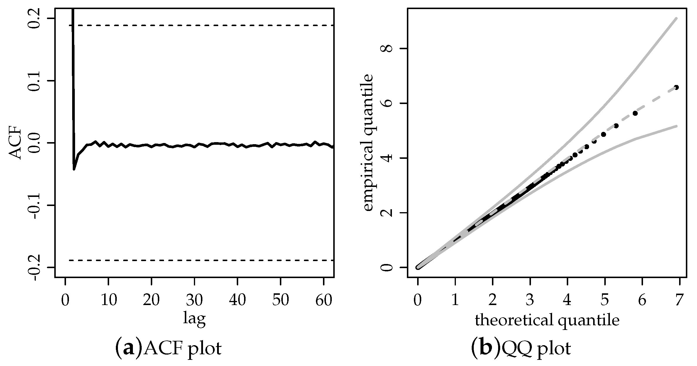
We now carry out an MC simulation study to examine the performance of the Cox–Snell residual $r^{\mathrm{cs}}$ defined in (22). To do so, we use the estimation procedure presented in Section 5.1 and consider only the BS-PE-ACD model, as it provides greater flexibility in relation to other models, that is, it has either less or greater (lighter or heavier tails) than the BS distribution. The BS-PE-ACD samples are generated using the transformation in (5). We simulate $B=1000$ MC samples of size $n=500$. The empirical autocorrelation function (ACF) of the residual $r^{\mathrm{cs}}$ is plotted in Figure 1a. This plot indicates that the BS-PE-ACD model is well specified, since the residual $r^{\mathrm{cs}}$ mimics a sequence of independent and identically distributed RVs and there is no indication of serial correlation. Moreover, the empirical mean of the residual $r^{\mathrm{cs}}$, whose value was expected to be 1, was 0.9836. Finally, using a quantile-against-quantile (QQ) plot with a simulated envelope (see Figure 1b), we note that the Cox–Snell residual has an excellent agreement with the EXP(1) distribution, which supports the adequacy and flexibility of the BS-PE-ACD model. It is then possible to conclude that the residual $r^{\mathrm{cs}}$ seems adequate to assess the adjustment of the proposed models.

Figure 1. Autocorrelation function (ACF) plot and quantile-against-quantile (QQ) plot with envelope for the residuals.

6. Application to Analysis of Financial Transaction Data

In this section, our objective is to assess the GBS-ACD and GBS-AACD models using TD data. In particular, we consider here three TD data sets studied in Bhatti (2010), corresponding to the time elapsed (in seconds) between two consecutive transactions, which cover forty trading days from January 1, 2002 to February 28, 2002: International Business Machines (IBM), Johnson and Johnson Company (JNJ), and The Proctor and Gamble Company (PG). Note that, as mentioned before, these types of data exhibit some diurnal patterns, so that the final data sets are constructed from adjusted TD ${\overline{x}}_i=x_i/\widehat{\varphi }$, where $\widehat{\varphi }=exp\left(\widehat{s}\right)$ and $\widehat{s}$ denotes a set of quadratic functions and indicator variables for each half-hour interval of the trading day from 9:30 am to 4:00 pm; for more details, see Giot (2000), Tsay (2002), and Bhatti (2010).

6.1. Exploratory Data Analysis

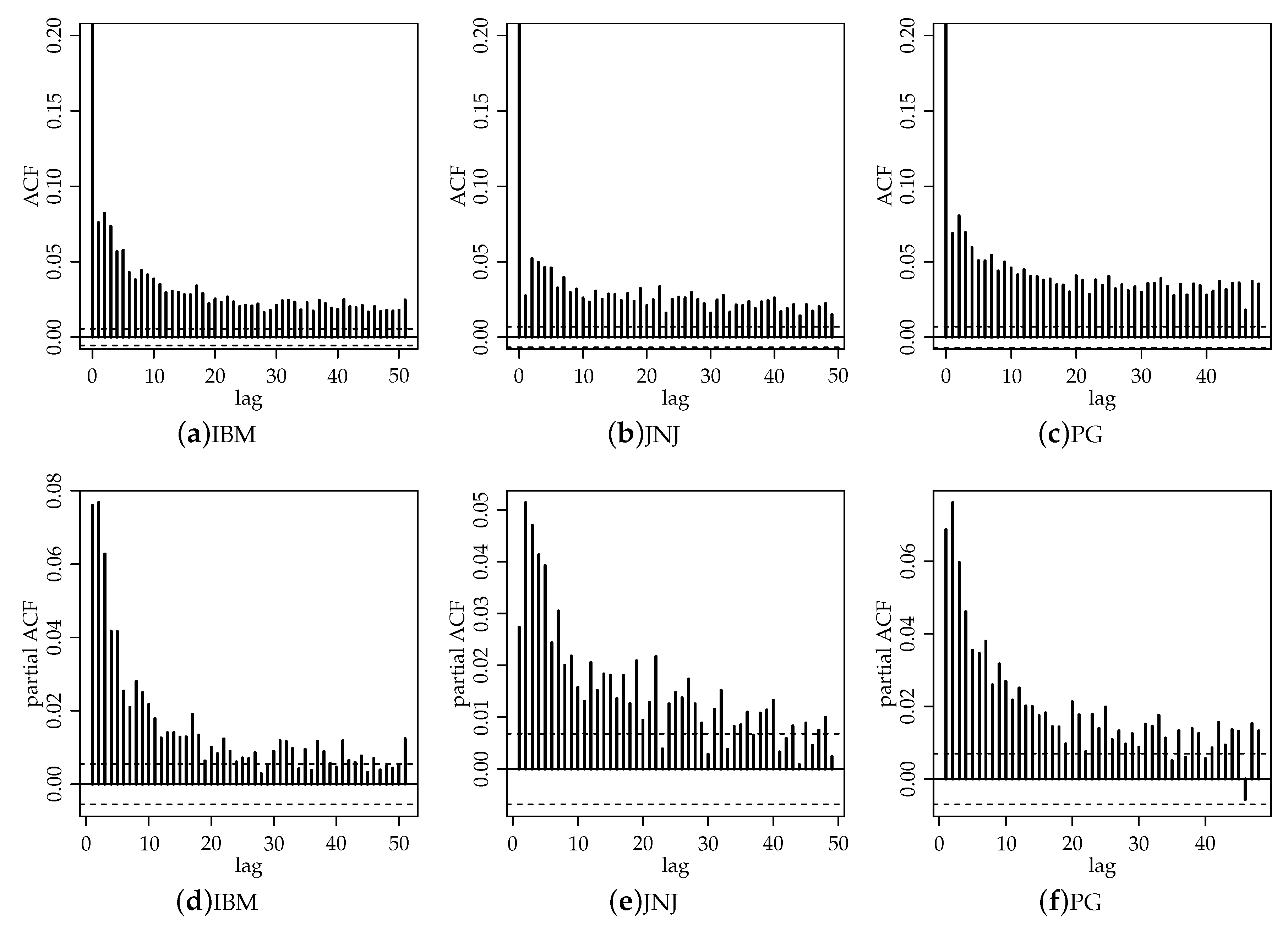
Table 3 provides some descriptive statistics for both plain and diurnally adjusted TD data, which include central tendency statistics and coefficients of variation (CV), of skewness (CS), and of kurtosis (CK), among others. These measures indicate the positively skewed nature and the high kurtosis of the data. Figure 2 shows graphical plots of the ACF and partial ACF for the IBM, JNJ, and PG data sets, which indicate the presence of serial correlation.

Table 3. Summary statistics for the International Business Machines (IBM), Johnson and Johnson Company (JNJ), and The Proctor and Gamble Company (PG) data sets.

	Data	Min.	Max.	Median	Mean	SD	CV	CS	CK
Plain data	IBM	1	166	5	6.768	6.234	92.10%	3.106	20.368
	JNJ	1	225	7	10.391	11.737	109.45%	3.187	18.706
	PG	1	172	7	10.904	12.066	110.66%	2.973	14.339
Adjusted data	IBM	0.169	32.523	1.038	1.384	1.252	90.43%	3.023	19.802
	JNJ	0.131	33.973	0.976	1.557	1.680	107.91%	3.135	18.463
	PG	0.121	26.327	0.985	1.582	1.718	108.58%	2.865	13.311

Figure 2. Autocorrelation and partial autocorrelation functions for the indicated data sets.

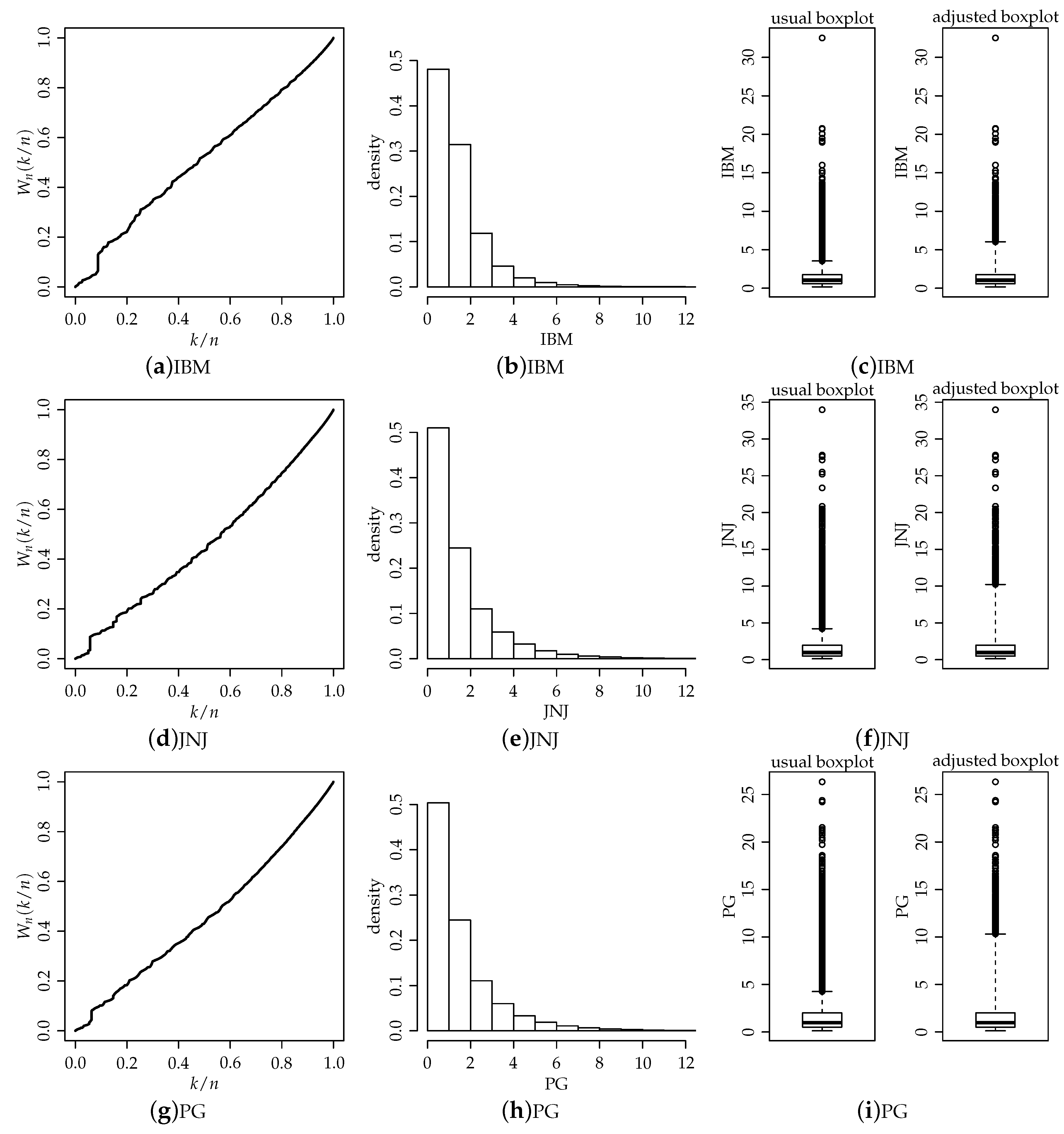
The hazard function of a positive RV X is given by $h_X\left(t\right)=f_X\left(x\right)/(1-F_X\left(x\right))$, where $f_X(·)$ and $F_X(·)$ are the PDF and CDF of X, respectively. A useful way to characterize the hazard function is by the scaled total time on test (TTT) function, namely, we can detect the type of hazard function that the data have and then choose an appropriate distribution. The TTT function is given by $W_X\left(u\right)=H_X^{-1}\left(u\right)/H_X^{-1}\left(1\right)$ for $0\le u\le 1$, where $H_X^{-1}\left(u\right)={\int }_0^{F_X^{-1}\left(u\right)}[1-F_X\left(y\right)]\mathrm{d}y$, where $F_X^{-1}(·)$ is the inverse CDF of X. By plotting the consecutive points $(k/n,W_n(k/n))$ with $W_n(k/n)=[{\sum }_{i=1}^k{x}_{\left(i\right)}+(n-k)x_k]/{\sum }_{i=1}^n{x}_{\left(i\right)}$ for $k=0,\dots ,n$, and $x_{\left(i\right)}$ being the ith-order statistic, it is possible to approximate $W_X(·)$; see Aarset (1987) and Azevedo et al. (2012).

From Figure 3, we observe that the TTT plots suggest a failure rate with a unimodal shape. We also observe that the histograms suggest a positive skewness for the data density. This supports the results obtained in Table 3. However, Huber and Vanderviere (2008) pointed out that, in cases where the data follow a skewed distribution, a significant number of observations can be classified as atypical when they are not. The boxplots depicted in Figure 3 suggest such a situation, i.e., most of the observations considered as potential outliers by the usual boxplot are not outliers when we consider the adjusted boxplot.

Figure 3. Total time on test (TTT) plot (a), histogram (b), and usual and adjusted boxplots (c) for the indicated data sets.

6.2. Estimation Results and Analysis of Goodness-of-Fit for the GBS-ACD Models

We now estimate the GBS-ACD models by the maximum likelihood method using the steps described in Section 5.1. Table 4, Table 5 and Table 6 present the estimation results for the indicated models. The standard errors (SEs) are reported in parentheses and ℓ stands for the value of the log-likelihood function, whereas $AIC=-2\ell +2k$ and $BIC=-2\ell +klnn$ denote, respectively, the Akaike information and Bayesian information criteria, where k stands for the number of parameters and n for the number of observations. The maximum and minimum values of the sample autocorrelations (ACF) from order 1 to 60 are also reported. Finally, $\overline{\gamma }$ denotes the mean magnitude of autocorrelation for the first 15 lags, namely, $\overline{\gamma }=1/15{\sum }_{i=1}^{15}\left|{\gamma }_k\right|$, where ${\gamma }_k=\mathrm{cor}(x_i,x_{i+k})$. The mean magnitude of autocorrelation $\overline{\gamma }$ is relevant for separating the influence of the sample size on the measure of the degree of autocorrelation in the residuals.

Table 4. Estimation results based on the generalized Birnbaum–Saunders autoregressive conditional duration (GBS-ACD) models for IBM trade durations.

	BS-ACD	BS-LA-ACD	BS-L0-ACD	BS-PE-ACD	BS-t-ACD
$\alpha$	−0.0454	−0.0495	−0.0503	−0.0473	−0.0470
	(0.00164)	(0.00199)	(0.00174)	(0.00168)	(0.00168)
$\beta$	0.9393	0.9387	0.9367	0.9373	0.9383
	(0.00381)	(0.00436)	(0.00389)	(0.00389)	(0.00384)
$\gamma$	0.0324	0.0385	0.0372	0.0342	0.0336
	(0.00116)	(0.00158)	(0.00128)	(0.00121)	(0.00119)
$\kappa$	0.8736	0.6862	0.4949	0.7934	0.8575
	(0.00173)	(0.00192)	(0.00115)	(0.00532)	(0.00266)
$\eta$				0.9019	54.4022
				(0.00582)	(7.05075)
ℓ	−153644.7	−157875.7	−154274.3	−153519.2	−153625.1
AIC	307297.4	315759.4	308556.6	307048.4	307260.2
BIC	307336.4	315798.4	308595.6	307097.2	307309
max ACF	0.0253	0.0293	0.0258	0.0341	0.0251
min ACF	−0.0075	−0.0100	−0.0089	−0.0052	−0.0079
$\overline{\gamma }$	0.0060	0.0061	0.0057	0.0074	0.0059

Table 5. Estimation results based on the GBS-ACD models for JNJ trade durations.

	BS-ACD	BS-LA-ACD	BS-L0-ACD	BS-PE-ACD	BS-t-ACD
$\alpha$	−0.0174	−0.0168	−0.0503	−0.0174	−0.0179
	(0.00080)	(0.00070)	(0.00174)	(0.00081)	(0.00078)
$\beta$	0.9744	0.9830	0.9367	0.9744	0.9769
	(0.00207)	(0.00138)	(0.00389)	(0.00209)	(0.00171)
$\gamma$	0.0113	0.0108	0.0372	0.0113	0.0115
	(0.00051)	(0.00044)	(0.00128)	(0.00051)	(0.00050)
$\kappa$	1.0427	0.8296	0.4949	1.0195	1.0395
	(0.00256)	(0.00288)	(0.00115)	(0.00749)	(0.00256)
$\eta$				0.9747	334.0810
				(0.00755)	(12.93302)
ℓ	−112581.4	−116353.4	−154274.3	−112575.8	−112582.8
AIC	225170.8	232714.8	308556.6	225161.6	225175.6
BIC	225208.1	232752.1	226547.4	225208.3	225222.1
max ACF	0.0197	0.0191	0.0182	0.0157	0.0189
min ACF	−0.0103	−0.0144	−0.0134	−0.0111	−0.0112
$\overline{\gamma }$	0.0075	0.0071	0.0072	0.0061	0.0070

Table 6. Estimation results based on the GBS-ACD models for PG trade durations.

	BS-ACD	BS-LA-ACD	BS-L0-ACD	BS-PE-ACD	BS-t-ACD
$\alpha$	−0.0182	−0.0313	−0.0181	−0.0189	−0.0231
	(0.00066)	(0.00281)	(0.00086)	(0.00070)	(0.00101)
$\beta$	0.9859	0.9744	0.9748	0.9856	0.9810
	(0.00101)	(0.00396)	(0.00223)	(0.00105)	(0.00150)
$\gamma$	0.0115	0.0202	0.0117	0.0120	0.0146
	(0.00041)	(0.00180)	(0.00055)	(0.00044)	(0.00063)
$\kappa$	1.0636	0.8404	0.5944	1.0058	1.0596
	(0.00267)	(0.00299)	(0.00171)	(0.00814)	(0.00286)
$\eta$				0.9401	267.2753
				(0.00770)	(67.87919)
ℓ	−108461.2	−111511.8	−113251	−108433	−108464.8
AIC	216930.4	223031.6	226510	216876	216939.6
BIC	216967.5	223068.7	218064	216922.4	216986.1
max ACF	0.0396	0.0309	0.0341	0.0326	0.0352
min ACF	−0.0143	−0.0133	−0.0140	−0.0101	−0.0132
$\overline{\gamma }$	0.0112	0.0067	0.0080	0.0114	0.0087

From Table 4, Table 5 and Table 6, we observe that all of the parameters are statistically significant at the $1\%$ level. It is also interesting to observe that, in general, the ACD parameter estimates are very similar across the models independently of the assumed distribution. In terms of AIC values, the BS-PE-ACD model outperforms all other models. Based on the BIC values, we note that the BS-PE-ACD model once again outperforms the remaining models, except for the JNJ data set. However, in this case, there does not exist one best model, since the BIC values for the BS-ACD and BS-PE-ACD models are very close.

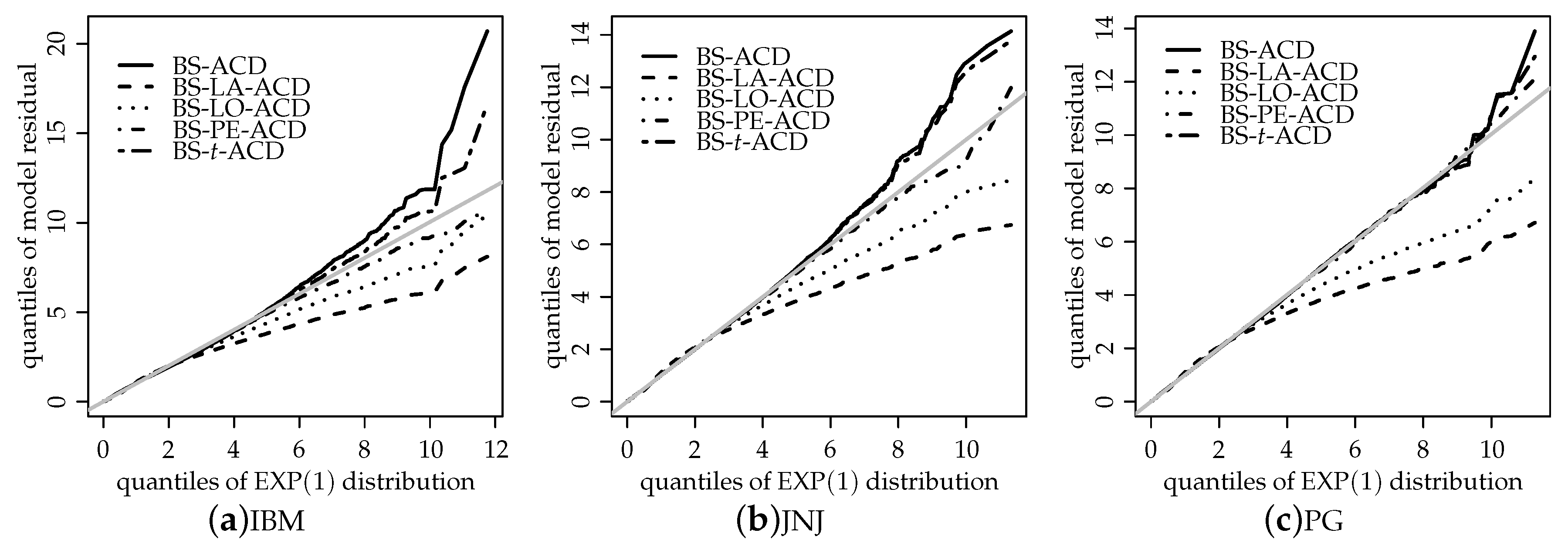
In order to check for misspecification, we look at the sample ACF from order 1 to 60. Table 4, Table 5 and Table 6 report that there is no sample autocorrelation greater than $0.05$ (in magnitude) throughout the models and residuals. Figure 4 shows the QQ plots of the Cox–Snell residual with the IBM, JNJ, and PG data sets. The QQ plot allows us to check graphically if the residual follows the $EXP\left(1\right)$ distribution. These graphical plots show an overall superiority in terms of fit of the BS-PE-ACD model. Moreover, the empirical means of the residual $r^{\mathrm{cs}}$ for the BS-PE-ACD model with the IBM, GM, and PG data sets were 1.0271, 0.9990, and 1.0153, respectively. Thus, the BS-PE-ACD model seems to be more suitable for modeling the data considered. It must be emphasized that this model provides greater flexibility in terms of kurtosis compared to the BS-ACD model.

Figure 4. QQ plot for the Cox–Snell residual with the indicated data sets.

6.3. Estimation Results for the BS-PE-AACD Models

We estimate here different ACD specifications (see Section 4) assuming a BS-PE PDF and using JNJ TD data. We focus on the BS-PE-AACD models (in short, AACD models), since, as observed in Section 6.2, this model fits the data adequately to provide effective ML-based inference. The estimation is performed using the steps presented in Section 5.1.

Table 7 and Table 8 report the estimation results for different specifications. It is important to point out that the estimates of the BS-PE parameters $\kappa$ and $\eta$ are quite robust throughout the specifications. The Box-Cox ACD result (see column BCACD) shows that allowing $\nu$ of ${\phi }_{i-1}$ to freely vary in the logarithm ACD processes (LACD I and LACD II) increases the log-likelihood value, indicating that $\nu$ may play a role. In fact, $\widehat{\nu }$ is significantly different from zero and one, thus supporting the BCACD model against its logarithm counterparts, i.e., LACD I and LACD II. The AIC values show that the BCACD, LACD I, and AACD are best models. From the BIC values, the LACD I, BCACD, and AACD models are the best ones. Note, however, that the BIC values for the LACD I and BCACD models are quite close. Table 4, Table 5 and Table 6 also show that there is no sample autocorrelation greater than $0.05$ (in magnitude) throughout the models and residuals.

Table 7. Estimation results for ACD specifications of JNJ trade durations. A star $(*)$ indicates that the parameter estimate is not significantly different from zero.

	LACD I	LACD II	BCACD	PACD
$\alpha$	7.2771e-05	−0.0174	−0.2719	0.0449
	(0.00165)	(0.00126)	(0.06500)	(0.01096)
$\beta$	0.9638	0.9744	0.9817	0.9266
	(0.02594)	(0.00294)	(0.00464)	(0.01604)
$\gamma$	0.0189	0.0113	0.2713	0.0258
	(0.00166)	(0.00081)	(0.06526)	(0.00893)
$\lambda$				0.4606 *
				(0.40488)
$\nu$			0.0713
			(0.02436)
$\kappa$	1.0190	1.0195	1.0189	1.0126
	(0.01245)	(0.00753)	(0.00748)	(0.00752)
$\eta$	0.9746	0.9747	0.9748	0.9678
	(0.03448)	(0.00758)	(0.00753)	(0.00754)
ℓ	−112544.7	−112575.8	−112539.5	−112558.6
AIC	225099.4	225161.6	225091	225129.2
BIC	225146	225208.3	225146.9	225185.1
max ACF	0.0175	0.0156	0.0158	0.0119
min ACF	−0.0130	−0.0113	−0.0134	−0.0188
$\overline{\gamma }$	0.0057	0.0061	0.0055	0.0045

Table 8. Estimation results for ACD specifications of JNJ trade durations. A star $(*)$ indicates that the parameter estimate is not significantly different from zero.

	A-ACD	A-LACD	A-PACD	AACD
$\alpha$	0.0267	−0.0167	0.1358	0.0319
	(0.00122)	(0.00344)	(0.00728)	(0.00881)
$\beta$	0.9537	0.9745	0.7975	0.8241
	(0.00601)	(0.00239)	(0.00077)	(0.00599)
$\gamma$	0.0139	0.0140	0.0632	0.1329
	(0.00100)	(0.00046)	(0.00918)	(0.00730)
$\lambda$			0.1118	0.5896
			(0.01008)	(0.08903)
$\nu$				0.1348
				(0.01590)
b	−0.1060 *	0.0610 *	−0.6393	−0.4250
	(0.69799)	(0.35477)	(0.21157)	(0.10707)
c	−0.1493	−0.1949	−0.1395 *	0.1229
	(0.05026)	(0.03656)	(1.82254)	(0.06525)
$\kappa$	1.0187	1.0195	1.0188	1.0182
	(0.00749)	(0.00749)	(0.00750)	(0.00749)
$\eta$	0.9740	0.9747	0.9737	0.9746
	(0.00754)	(0.00755)	(0.00755)	(0.00756)
ℓ	−112574.5	−112575.8	−112681.5	−112543.1
AIC	225163	225165.6	225379	225104.2
BIC	225228.3	225230.9	225453.6	225188.2
max ACF	0.0148	0.0157	0.0171	0.0137
min ACF	−0.0114	−0.0111	−0.0253	−0.0147
$\overline{\gamma }$	0.0057	0.0061	0.0081	0.0049

7. Concluding Remarks

We have introduced a general class of ACD models based on GBS distributions. These distributions possess either lighter or heavier tails than the BS distribution, thus providing a wider class of positively skewed densities with nonnegative support. In addition, we have proposed a wider class of GBS-ACD models based on the Box-Cox transformation with a shape parameter to the conditional duration process and an asymmetric response to shocks. We then investigated the performance of the maximum likelihood estimates of the GBS-ACD models by means of an MC study. We also compared the proposed GBS-ACD and GBS-AACD models through an analysis with real financial data sets, which has shown the superiority of the BS-PE-ACD and BS-PE-BCACD models. A future line of research may be the out-of-sample forecast abilities of these models, as well as their application to other types of irregularly time-spaced data (besides TD data).

References

1. Aarset, M. V. 1987. How to identify a bathtub hazard rate. IEEE Trans. Rel. 36: 106–08. [Google Scholar] [CrossRef]
2. Allen, D., F. Chan, M. McAleer, and S. Peiris. 2008. Finite sample properties of the QMLE for the log-ACD model: Application to Australian stocks. J. Econometrics 147: 163–83. [Google Scholar] [CrossRef] [Green Version]
3. Azevedo, C., V. Leiva, E. Athayde, and N. Balakrishnan. 2012. Shape and change point analyses of the Birnbaum-Saunders-t hazard rate and associated estimation. Comp. Statist. Data Anal. 56: 3887–97. [Google Scholar] [CrossRef] [Green Version]
4. Barros, M., G. A. Paula, and V. Leiva. 2008. A new class of survival regression models with heavy-tailed errors: Robustness and diagnostics. Lifetime Data Anal. 14: 316–32. [Google Scholar] [CrossRef]
5. Bauwens, L., and P. Giot. 2000. The logarithmic ACD model: An application to the bid-ask quote process of three NYSE stocks. Ann. Econ. Statist. 60: 117–49. [Google Scholar] [CrossRef]
6. Bauwens, L., and P. Giot. 2003. Asymmetric ACD models: Introducing price information in ACD models. Empir. Econ. 28: 709–31. [Google Scholar] [CrossRef]
7. Bhatti, C. R. 2010. The Birnbaum-Saunders autoregressive conditional duration model. Math. Comp. Simul. 80: 2062–78. [Google Scholar] [CrossRef]
8. Bhogal, S. K., and R. Variyam Thekke. 2019. Conditional duration models for high-frequency data: A review on recent developments. J. Econ. Surv. 33: 252–73. [Google Scholar] [CrossRef] [Green Version]
9. Birnbaum, Z. W., and S. C. Saunders. 1969. A new family of life distributions. J. Appl. Prob. 6: 319–27. [Google Scholar] [CrossRef]
10. Bollerslev, T. 1986. Generalized autoregressive conditional heteroskedasticity. J. Econometrics 31: 307–27. [Google Scholar] [CrossRef] [Green Version]
11. Box, G. E. P., and D. R. Cox. 1969. An analysis of transformations. J. R. Statist. Soc. B 26: 211–43. [Google Scholar] [CrossRef]
12. Chiang, M. 2007. A smooth transition autoregressive conditional duration model. Stud. Nonlinear Dyn. E. 11: 108–44. [Google Scholar] [CrossRef]
13. De Luca, G., and P. Zuccolotto. 2006. Regime-switching Pareto distributions for ACD models. Comp. Statist. Data Anal. 51: 2179–91. [Google Scholar] [CrossRef]
14. Diamond, D. W., and R. E. Verrechia. 1987. Constraints on short-selling and asset price adjustments to private information. J. Finan. Econ. 18: 277–311. [Google Scholar] [CrossRef]
15. Díaz-García, J. A., and J. R. Domínguez-Molina. 2006. Some generalisations of Birnbaum-Saunders and sinh-normal distributions. Int. Math. Forum 1: 1709–27. [Google Scholar] [CrossRef] [Green Version]
16. Díaz-García, J. A., and V. Leiva. 2005. A new family of life distributions based on the contoured elliptically distributions. J. Statist. Plann. Infer. 128: 445–57. [Google Scholar] [CrossRef]
17. Engle, R. F. 1982. Autoregressive conditional heteroscedasticity with estimates of the variance of United Kingdom inflation. Econometrica 50: 987–1008. [Google Scholar] [CrossRef]
18. Engle, R., and J. Russell. 1998. Autoregressive conditional duration: A new method for irregularly spaced transaction data. Econometrica 66: 1127–62. [Google Scholar] [CrossRef]
19. Easley, D., and M. O’Hara. 1992. Time and the process of security price adjustment. The Journal of Finance 47: 577–605. [Google Scholar] [CrossRef]
20. Easley, D., N. M. Kiefer, and M. O’Hara. 1997. The information content of the trading process. Journal of Empirical Finance 4: 159–86. [Google Scholar] [CrossRef]
21. Fang, K. T., S. Kotz, and K. W. Ng. 1990. Symmetric Multivariate and Related Distributions. London: Chapman & Hall. [Google Scholar]
22. Fernandes, M., and J. Grammig. 2006. A family of autoregressive conditional duration models. J. Econometrics 130: 1–23. [Google Scholar] [CrossRef] [Green Version]
23. Ghosh, Y. N., and B. Mukherjee. 2006. On probabilistic properties of conditional median and quantiles. Statist. Prob. Letters 76: 1775–80. [Google Scholar] [CrossRef]
24. Giot, P. 2000. Time transformations, intraday data and volatility models. J. Comp. Finance 4: 31–62. [Google Scholar] [CrossRef] [Green Version]
25. Grammig, J., and K. Maurer. 2000. Non-monotonic hazard functions and the autoregressive conditional duration model. Economet. J. 3: 16–38. [Google Scholar] [CrossRef]
26. Hubert, M., and E. Vandervieren. 2008. An adjusted boxplot for skewed distributions. Comp. Statist. Data Anal. 52: 5186–201. [Google Scholar] [CrossRef]
27. Jasiak, J. 1998. Persistence in intertrade durations. Finance 19: 166–95. [Google Scholar] [CrossRef] [Green Version]
28. Leiva, V., M. Barros, G. A. Paula, and A. Sanhueza. 2008. Generalized Birnbaum-Saunders distributions applied to air pollutant concentration. Environmetrics 19: 235–49. [Google Scholar] [CrossRef]
29. Leiva, V., H. Saulo, J. Leão, and C. Marchant. 2014. A family of autoregressive conditional duration models applied to financial data. Comp. Statist. Data Anal. 79: 175–91. [Google Scholar] [CrossRef]
30. Lunde, A. 2008. A Generalized Gamma Autoregressive Conditional Duration Model. Discussion Paper. Denmark: Aalborg University. [Google Scholar]
31. Marchant, C., K. Bertin, V. Leiva, and H. Saulo. 2013. Generalized Birnbaum-Saunders kernel density estimators and an analysis of financial data. Comp. Statist. Data Anal. 63: 1–15. [Google Scholar] [CrossRef]
32. Mayorov, K. 2011. Modelling Trade Durations with the Birnbaum-Saunders Autoregressive Model. M.Sc. thesis, McMaster University, Hamilton, ON, Canada. [Google Scholar]
33. Nelder, J. A., and R. Mead. 1965. A simplex method for function minimization. Comp. J. 7: 308–13. [Google Scholar] [CrossRef]
34. Pacurar, M. 2008. Autoregressive conditional durations models in finance: A survey of the theoretical and empirical literature. J. Econ. Surv. 22: 711–51. [Google Scholar] [CrossRef]
35. Pathmanathan, D., K. H. Ng, and M. S. S. Peiris. 2009. On estimation of autoregressive conditional duration (ACD) models based on different error distributions. S. Lankan J. Appl. Statist. 10: 251–69. [Google Scholar]
36. Rieck, J., and J. Nedelman. 1991. A log-linear model for the Birnbaum-Saunders distribution. Technometrics 33: 51–60. [Google Scholar]
37. Sanhueza, A., V. Leiva, and N. Balakrishnan. 2008. The generalized Birnbaum–Saunders distribution and its theory, methodology and application. Comm. Statist. Theor. Meth. 37: 645–70. [Google Scholar] [CrossRef]
38. Saulo, H., J. Leão, V. Leiva, and R. G. Aykroyd. 2019. Birnbaum-Saunders autoregressive conditional duration models applied to high-frequency financial data. Stat. Pap. 60: 1605–29. [Google Scholar] [CrossRef] [Green Version]
39. Saunders, S. C. 1974. A family of random variables closed under reciprocation. J. Amer. Statist. Assoc. 69: 533–39. [Google Scholar] [CrossRef]
40. Tsay, R. S. 2002. Analysis of Financial Time Series. New York: John Wiley & Sons. [Google Scholar]
41. Zhang, M. Y., J. R. Russell, and R. S. Tsay. 2001. A nonlinear autoregressive conditional duration model with applications to financial transaction data. J. Econometrics 104: 179–207. [Google Scholar] [CrossRef]