Regime-Dependent Good and Bad Volatility of Bitcoin


1
Indian Institute of Technology (IIT) Kanpur, Uttar Pradesh 208016, India
2
Business School, University of Western Australia, Perth, WA 6009, Australia
*
Author to whom correspondence should be addressed.
J. Risk Financial Manag. 2020, 13(12), 312; https://doi.org/10.3390/jrfm13120312
Submission received: 8 October 2020
/
Revised: 1 December 2020
/
Accepted: 2 December 2020
/
Published: 7 December 2020
(This article belongs to the Special Issue Recent Developments in Cryptocurrency Markets: Co-movements, Spillovers and Forecasting)
Abstract
:This paper analyzes high-frequency estimates of good and bad realized volatility of Bitcoin. We show that volatility asymmetry depends on the volatility regime and the forecast horizon. For one-day ahead forecasts, good volatility commands a stronger impact on future volatility than bad volatility on average and in extreme volatility regimes but not across all quantiles and volatility regimes. For 7-day ahead forecasting horizons the asymmetry is similar to that observed in stock markets and becomes stronger with increasing volatility. Compared with stock markets, the persistence and predictability of volatility is low indicating high variations of volatility.
Keywords:
semivariance; bitcoin; volatility asymmetry; high-frequency data; HAR; quantile regression1. Introduction
It is a well-known fact that Bitcoin prices fluctuate significantly. This excess volatility of Bitcoin (e.g., see Yermack 2013) potentially makes volatility forecasting more difficult and highlights the importance of volatility forecasting for risk management. In addition, volatility forecasting can identify drivers of volatility and thus lead to a deeper understanding of volatility and the characteristics of the asset. Since news shocks are key drivers of volatility, we focus on such shocks and analyze the influence of shocks on future volatility and whether there are differences and thus an asymmetry between positive shocks and negative shocks, across return frequencies and across volatility regimes.
A study of the predictability of Bitcoin returns is also important to shed more light on the relationship between excess volatility and volatility persistence implying predictability. A high or excess volatility may be less of a problem if it is predictable to a certain degree compared to a situation in which high volatility is not predictable and volatility fluctuates between high volatility states and lower volatility states.
This paper is motivated by the excess volatility of Bitcoin and employs a heterogeneous autoregressive–realized volatility–quantile regression model (HAR-RV-QR) to estimate the role of positive and negative shocks on future volatility, the persistence and predictability of volatility across different data frequencies (HAR) and for different levels of volatility (QR).
A comparison of the results with empirical studies based on equity markets can help to identify significant differences of the crypto market with the equity market and enhance our understanding of Bitcoin and crypto assets in general. For example, the separation of daily shocks into daily positive shocks and daily negative shocks helps to predict future volatility of equity returns (Patton and Sheppard 2015) but it is not clear how important this separation is to predict the volatility of Bitcoin. Given Bitcoin’s excess volatility, it is well possible that volatility is less predictable and that the separation of shocks into positive and negative shocks is less useful. The predictability may also depend on the levels of volatility which is assessed in a quantile regression framework. Baur and Dimpfl (2018b) found for equity returns that volatility asymmetry and volatility persistence are high volatility phenomena only and not present in low volatility regimes. It is interesting to understand whether this finding also holds for Bitcoin despite or because of its excess volatility.
The literature on cryptocurrencies has been growing fast since the introduction of Bitcoin (Nakamoto (2008)) and the study by Yermack (2013). Recent work on the volatility of Bitcoin and cryptocurrencies includes Baur et al. (2018); Katsiampa (2017); Katsiampa et al. (2019) and Kyriazis et al. (2020). Mensi et al. (2019) use high-frequency data and semivariances but focus on spillovers. Shen et al. (2020) present an analysis of different forecasting models for Bitcoin.
It is a well-established fact that volatility associated with negative returns increases the future volatility by more than the volatility associated with positive returns for various assets at different frequencies (Bekaert and Wu (2000); Christie (1982); French et al. (1987)). This asymmetry is mainly explained by the leverage effect and the volatility feedback effect for equity markets. A commonly used framework to estimate asymmetric effects is through a GARCH-type model such as the asymmetric GARCH model by Glosten et al. (1993).
In contrast to the equity market, studies on the asymmetric volatility effect are less abundant in the Bitcoin market. Bouri et al. (2017) use a GARCH model to identify an inverse asymmetric return-volatility effect in the Bitcoin market prior to the Bitcoin price crash in 2013 and no significant relation thereafter. Baur and Dimpfl (2018a) detect inverted asymmetric volatility effects in a sample of 20 large cryptocurrencies. The authors follow Avramov et al. (2006) and explain their findings with trading activity of uninformed noise traders for positive shocks and trading activity of informed traders for negative shocks. Cheikh et al. (2020) analyzes the presence of inverted asymmetric volatility in the Bitcoin market using a Smooth Transition GARCH model. They find that positive shocks increase volatility by more than the negative shocks confirming the inverted asymmetric volatility effect. They attribute this positive return–volatility relationship to the possible hedging and safe haven property of Bitcoin.
However, most studies that analyze asymmetric volatility use daily data and do not exploit the information embedded in intraday prices or do not allow phenomena such as volatility asymmetry to depend on the level of volatility.
This paper addresses these issues by employing a HAR-RV-QR model to analyze the importance of realized semivariance in affecting the future volatility in the Bitcoin market. The HAR-RV models are not only useful in studying the predictability of future volatility but also in exploring the asymmetric volatility effect using high-frequency data. Decomposition of realized volatility into good volatility (arising from positive returns) and bad volatility (arising from negative returns) helps to understand the relative importance of positive and negative semivariance in affecting future volatility.
Patton and Sheppard (2015) use a HAR-RV model to show that future volatility increases by more in response to past negative returns than to past positive returns for stock indices and individual US stocks. Todorova (2017) uses a similar model to identify an inverted asymmetric effect for gold, i.e., positive shocks increase volatility by more than negative shocks.
The main findings of this study based on high-frequency data are consistent with the existing literature based on daily data (e.g., see Baur and Dimpfl (2018a)). However, the HAR-RV-QR reveals that the inverted asymmetric effect only holds for specific volatility regimes and is thus dependent on the quantiles of volatility. This result is in contrast to Baur and Dimpfl (2018b) who analyze stock market indices and find that volatility asymmetry is a high-volatility phenomenon and that there is no asymmetry in low or medium volatility periods. The finding that volatility asymmetry is not a high volatility phenomenon highlights the different volatility dynamics of Bitcoin relative to equity markets.
The results also show that the predictability is lower than for equity markets and decreases substantially over longer horizons. This finding may not be surprising given the excess volatility of Bitcoin but it emphasizes the differences between excess volatility and persistence.
2. Data and Methodology
The data includes Bitcoin prices at 5-min frequency from the Bitstamp (USD) exchange, and is extracted from Bitcoincharts.com over five years from 01/01/2015 to 31/12/2019. We omit days with more than 40% of missing observations resulting in 1821 days and 524,448 observations.
2.1. Realized Volatility, Continuous and Signed Jump Processes
The quadratic variation of a continuous-time stochastic process for log prices, , consisting of a continuous and a jump component is given by
where captures the jump. Andersen et al. (2001) introduced realized variance given as
where .
Barndorff-Nielsen and Shephard (2004) used bipower variation (BV) to estimate the continuous part of the price process as follows
Barndorff-Nielsen et al. (2008) split realized variance into upside and downside realized semivariance, which captured variation due to positive and negative returns respectively. These estimators are defined as
We also use the signed jump variation defined by Patton and Sheppard (2015) as . The difference eliminates the common integrated variance term and is positive when a day is dominated by positive shocks and negative if a day is dominated by negative shocks. Using signed jump instead of jump (RV − BV), gives the advantage of studying the impact of positive and negative jumps on future volatility separately.
2.2. Econometric Modelling
The econometric analysis is based on the following Heterogeneous Auto-Regressive–Realized Volatility (HAR-RV) models first introduced by Corsi (2009).
Model 1:
Model 2:
Model 3:
Model 4:
Model 5:
The models are estimated for one-day, and one-week ahead horizons ( and ). We do not use since the Bitcoin market has continuous 7-day trading. Model 1 presents a basic realized volatility model and model 2 is an expanded version with the daily realized volatility separated into a positive and negative semivariance. Model 3 uses the bipower variation as an alternative to model 1 and model 4 is an augmented version including the signed jump variation. If decomposing RV into RS and RS adds no extra information, we expect = and thus no asymmetric volatility effect. However, if < , the “classical” (equity-like) volatility asymmetry is found with negative returns having a stronger impact on future volatility than positive returns Patton and Sheppard (2015). Similarly, if > , the upside semivariance (“Good Volatility”) has a higher impact on future volatility than the downside semivariance ("Bad Volatility") resulting in an inverted asymmetry effect.
Further, model 5 is an augmented version of model 2 and includes the realized variance interacted with an indicator for negative returns, , motivated by the interaction term used in the asymmetric GARCH model of Glosten et al. (1993). If realized semivariance adds no new information beyond the interaction variable, we expect = and to be significant.
Since “estimation by OLS has the unfortunate feature that the resulting estimates focus primarily on fitting periods of high variance and place little weight on more tranquil periods” (Patton and Sheppard (2015), page 687), we use quantile regression (QR) to mitigate this feature.1 More specifically, we use a HAR-RV-QR model to investigate if ordinary least squares (OLS) regression under- or over-estimates the importance of upside or downside semivariances in forecasting the future volatility. This model gives us an idea in which way volatility asymmetry, if present, is dependent on the quantile of the realized volatility. We use the HAR-RV-QR specification for model 2 as follows
where and denotes the conditional quantile of the realized volatility conditional on the regressor variables for quantile . We estimate 95 quantiles from the 3% quantile up to the 97% quantile to obtain a precise picture of the relationships across different quantiles. Inference is based on bootstrapped standard errors.
We follow Koenker and Bassett (1978) and use the L1-weighted loss function to obtain estimates of the parameters in Equation (6), i.e., we solve the minimization problem
where is the tilted absolute value function, namely
It is important to note that our quantile-based forecasts are conditional on the quantiles and thus only allow forecasts of the future distribution of volatility. In other words, since we do not know tomorrow’s volatility regime (quantile) we cannot forecast tomorrow’s volatility but only the distribution of future volatility.
3. Estimation Results
Figure 1 presents time-series plots of the continuous component of volatility (BV), signed jumps and the price of Bitcoin, and a scatter plot illustrating the relationship between good and bad volatility. The Figure illustrates that the jump component is significantly smaller than the continuous (BV) component and dominated by bad volatility as most values are negative (recall that the signed jump is equal to good volatility minus bad volatility, i.e., ).
The scatter plot of good and bad volatility further shows that “good” and “bad” volatility days are not exclusive but frequently occur on the same days and that extreme bad volatility is greater than extreme good volatility.
Table 1 presents the summary statistics for the various volatility measures and confirms that bad volatility is larger than good volatility. The numbers also show that the maximum positive semivariance (3.578) and the maximum negative semivariance (7.782) fell on the same day since the minimum jump is −4.204 which is the difference of the two semivariances (3.578 − 7.782 = −4.205). This confirms the relationship for extreme realizations. The relationship also holds for the mean values (0.106 − 0.119 = −0.012).
The bottom panel contains the correlation between different volatility measures. The correlation between and , at around 88%, is markedly lower than the correlation between the semivariances and either RV or BV, indicating that there is novel information in this decomposition.
3.1. Heterogeneous Autoregressive (HAR) Model
The estimation results of models 1–4 are presented in Table 2 and show that the coefficients for good and bad volatility differ from each other and from the daily component of realized volatility. A test of the equality of the coefficients further shows that the coefficients of good and bad volatility are indeed significantly different from each other. The null is rejected at the 5% level with an F-statistic of 5.456. This means that disentangling the daily component of realized volatility into its components provides additional information. A comparison of model 1 with model 2 shows that daily realized volatility averages the effect of positive and negative realized semivariance. However, despite the statistically significant difference in the coefficient estimates, the semivariances only marginally increase the from 0.321 to 0.323.
Model 2 further shows that good volatility has a stronger impact on future volatility than bad volatility which is in stark contrast to the volatility asymmetry generally identified in equity markets (Patton and Sheppard (2015)) but similar to gold (Todorova (2017)) and consistent with other studies on Bitcoin (e.g., Baur and Dimpfl (2018a)).
The coefficient of the signed jump variation in model 4 is not significantly different from zero which means that most of the future volatility is affected by the continuous component of realized volatility. A relatively high value of the coefficient of bipower variation confirms this.
Finally, model 5 shows that the coefficient estimate of the lagged interaction term is insignificant which implies that realized semivariances contain useful information for future volatility.
The estimation results for the 7-day ahead volatility forecasts presented in Table 3 have a significantly lower explanatory power, weaker volatility persistence and exhibit a very different, equity-like, volatility asymmetry. It seems that the inverted asymmetry identified for 1-day ahead forecasts is a short-run phenomenon and converges to the “classic” asymmetry over longer horizons. A similar effect is observed for the jump component which becomes significant for the 7-day ahead results but is insignificant for the 1-day ahead results.
The estimates of model 5 show that the interaction term is significantly negative but small. It is around 30% of the negative semivariance term. The increase in is also marginal. Moreover, the coefficients of good and bad volatility are statistically different from each other in the model. Thus, the results for one day and seven day horizons indicate that the semivariances capture the asymmetric impact of volatility in a better sense than the method of using an interaction term for lagged daily negative return.
Comparing the results for one day ahead volatility (0.642 for good volatility and 0.239 for bad volatility) with the results in Patton and Sheppard (2015) for stocks (0.183 for good volatility and 0.708 for bad volatility), shows that while future volatility increases with the volatility associated with the negative returns for stocks, the opposite is true for Bitcoin. This is in line with the existing literature. In addition, the improvement of R-squared with the inclusion of semivariances in our model is marginal and smaller than that reported in Patton and Sheppard (2015). This implies that a decomposition of realized volatility into its constituent components does not materially increase the predictability of future volatility in the Bitcoin market. The forecasting power for the week ahead (h = 7) volatility is significantly lower than that in Patton and Sheppard (2015) indicating that the volatility of Bitcoin is less persistent and thus less predictable than that of stocks.
This reversion of the asymmetric effect at to the “classical” effect is particularly interesting because there is no such change in the asymmetric effect in equity markets (e.g., Patton and Sheppard 2015). While the coefficient estimates weaken with increasing forecasting horizon in equity markets the effect does not change its sign across the entire set of horizons.
The changes in the asymmetric effect across forecast horizons imply that the drivers of volatility vary which supports the idea that volatility is both high and less predictable than the volatility of other assets.
3.2. HAR–QR Model
The Quantile Regression results are presented in Figure 2 and show that good volatility does not dominate bad volatility over the entire distribution but that the inverted asymmetry only holds for lower quantiles and extreme upper quantiles. Further, the joint test of equality of slopes yields an F-statistic of 319.49 indicating that the coefficients are significantly different from each other across all quantiles.
The QR estimates for weekly volatility are relatively constant over all quantiles with slightly weaker relationships at the extreme tails of the distribution. In contrast, the monthly volatility estimates increase significantly from low to high quantiles and appear to become significantly more important for high volatility regimes.
While the OLS estimates suggest that the positive semivariance is more important for future volatility than the negative semivariance, the quantile regression estimates indicate that the result is also dependent on the quantile of the realized volatility.
The quantile regression results for the 7-day ahead volatility presented in Figure 3 confirm the markedly different volatility asymmetry and lower volatility persistence on average and the significant differences across quantiles particularly for high quantiles relative to low and intermediate quantiles.
Figure 4 is intended to clarify the differences between the good and bad volatility estimates across quantiles for the 1-day and 7-day ahead horizons. While the importance of good and bad volatility appears unstable and changes across quantiles for the 1-day horizon, there is a clear trend in the importance and the difference between good and bad volatility for the 7-day horizon. Specifically, the difference widens substantially for increasing quantiles.
Over 1-day horizons, both good and bad volatility increase future volatility. Good volatility dominates in extreme quantiles, low quantiles and very high quantiles whereas bad volatility dominates in medium-low to medium-high quantiles. In other words, we observe both an inverted asymmetric effect and a classical equity-like asymmetry conditional on the quantiles of volatility. Over 7-day horizons, the classical equity-like asymmetry is present across the entire distribution. Bad volatility not only dominates good volatility but bad volatility increases future volatility and good volatility decreases future volatility.
Our quantile regression results unravel an important aspect of Bitcoin volatility asymmetry, i.e., an unstable asymmetry switching between classical and inverted asymmetry dependent on the volatility regime and the forecast horizon. Our results contrast findings for the equity market (Baur and Dimpfl 2018b) that volatility asymmetry is only a high-volatility phenomenon.
Figure 5 and Figure 6 present the quantile regression results for the 1-day and 7-day horizons based on Model 4, respectively. Model 4 uses bipower variation and jump variation instead of good and bad volatility (as specified in Model 2). The coefficient estimates for the jump variation can be related to the previously discussed graphs and show patterns consistent with the difference between good and bad volatility, i.e., the jump variation is relatively stable across quantiles for the 1-day ahead horizon but clearly decreases for the 7-day ahead horizon. The results are intuitive since the jump variation is defined as the difference between good volatility and bad volatility.
Figure 7 and Figure 8 present the quantile regression results for the 1-day and 7-day horizons based on Model 5. The results are similar compared with the OLS results. The interaction term is close to zero and insignificant across all quantiles for the 1-day ahead horizon. For the 7-day ahead horizon, we find that the lagged interaction term is significantly negative but small across most quantiles except for very high quantiles for which the coefficients increase towards confirming the strong effect of negative shocks or bad volatility on future volatility as also reported in Figure 4.
3.3. Long-Horizon Forecasts and Predictive Power
This section extends the previous analysis and estimates the models for a larger and longer set of forecast horizons.
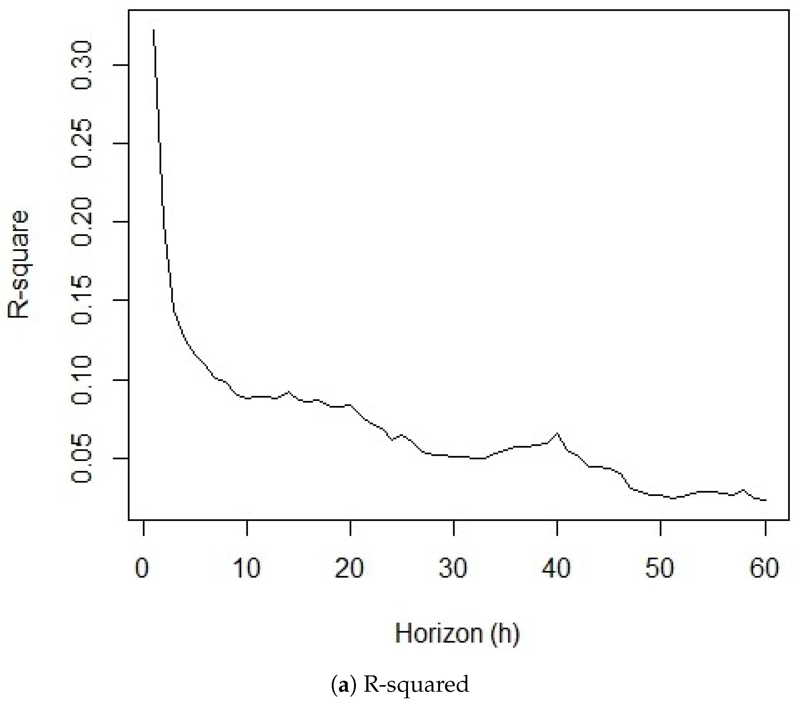
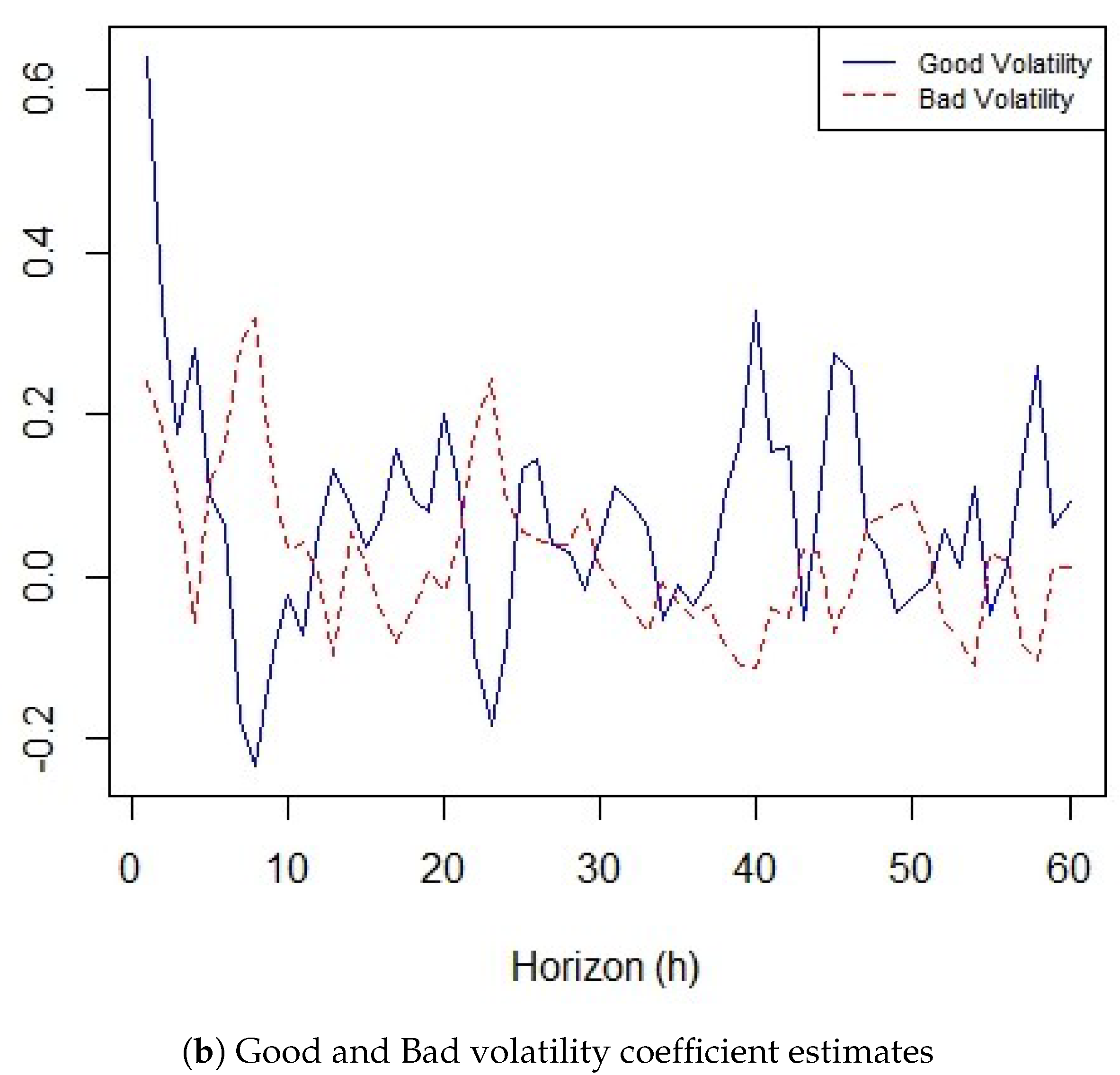
In line with Patton and Sheppard (2015), we extend our model to longer horizons to study the predictive power of the model. We find a decreasing predictive power for increasing forecast horizons. Figure 9a presents the R-squared values based on model 2 for all horizons from h = 1 to h = 60. There is a continuous decline in the R-squared values from 0.32 at h = 1 to 0.02 at h = 60. This is equivalent to a 94% drop in the R-squared value and is in stark contrast to Patton and Sheppard (2015) where the R-squared values drop from 0.61 to 0.31, at h = 66, a relative drop of about 50%. A plausible reason for this weaker forecasting power for increasing horizons in Bitcoin is the “excess” volatility in comparison to the equity market. The coefficient estimates become insignificant for increasing horizons and there is no clear pattern in the importance of good and bad volatility as shown in Figure 9b. The changing importance of good and bad volatility for different h supports our argument that volatility is not only high but that volatility of volatility is high and poor predictability is represented by an unstable and switching asymmetric effect.2
The unstable volatility asymmetry also has potential implications for Bitcoin’s role as a safe haven. If the inverted asymmetric volatility effect is related to a potential safe haven effect of Bitcoin as suggested by Bouri et al. (2019), the quantile regression results imply that such a safe haven property only holds in extreme volatility regimes (quantiles) but not in medium-low to medium-high volatility regimes. Such a conditional safe haven characteristic potentially adds to the evidence against Bitcoin’s safe haven property (e.g., see Klein et al. 2018 and Smales 2019).
3.4. Robustness
We separated the sample into two sub-samples, from 1 January 2015 to 4 July 2017 prior to the bubble-like price increase in 2017 and from 5 July 2017 to 31 December 2019.3 The sub-sample analysis reveals changes in the asymmetry over time consistent with the quantile regression estimates that identifies changes across quantiles. Specifically, for the first sub-sample we find an inverted asymmetry with a positive coefficient for good volatility and a negative coefficient for bad volatility, and for the second sub-sample we find a “classical” asymmetry with an insignificant coefficient for good volatility and a positive coefficient for bad volatility. The coefficient estimates for the lagged weekly and monthly volatility indicate a substantially higher persistence of volatility in the second sub-sample suggesting that Bitcoin became more stable compared with the first, earlier, sub-sample
4. Conclusions
This paper extended the existing literature on the volatility of Bitcoin with a separation of realized volatility into good and bad volatility, and into a continuous and a jump component within a HAR–QR framework. The results for 1-day ahead forecast horizons show that good volatility is more important in predicting future volatility than bad volatility on average but not in all volatility regimes. The results for the 7-day ahead forecast horizons reveal that the asymmetry resembles the typical effects observed in equity markets, i.e., bad volatility increases volatility by more than good volatility and the strength of the asymmetry increases with volatility. However, the predictability of future volatility is low compared with equity markets indicating that volatility is not merely high but that the volatility of volatility is high. The relatively poor predictive power of the models compared with the equity market and the unstable asymmetric volatility emphasize that “excess volatility” is an incomplete characterization of Bitcoin. Excess volatility is less of a problem if it is persistent and predictable. However, we find that volatility is not only excessively high but also volatile and the drivers of volatility do not have a stable influence over different volatility regimes.
The findings demonstrate that high-frequency data within a HAR and Quantile Regression framework provide deeper information that cannot be identified with lower frequency daily data and less sophisticated models.
The findings of this study may also have implications for the role of Bitcoin as a hedge. There is a large literature on the hedging properties of Bitcoin but the unstable nature of the drivers of volatility and volatility per se may undermine Bitcoin’s role as a hedge. For example, if the volatility is unstable, the correlation may also be unstable and destroy any advantageous hedging properties of Bitcoin against other assets.
Author Contributions
Conceptualization, K.K.J. 60% and D.G.B. 40%; methodology, K.K.J. 60% and D.G.B. 40%; software, K.K.J. 100% and D.G.B. 0%; validation, K.K.J. 50% and D.G.B. 50%; formal analysis, K.K.J. 50% and D.G.B. 50%; investigation, K.K.J. 50% and D.G.B. 50%; resources, K.K.J. 50% and D.G.B. 50%; data curation, K.K.J. 100%; writing—original draft preparation, K.K.J. 60% and D.G.B. 40%; writing—review and editing, K.K.J. 30% and D.G.B. 70%; visualization, K.K.J. 50% and D.G.B. 50%; supervision, K.K.J. 0% and D.G.B. 100%; project administration, K.K.J. 50% and D.G.B. 50%. All authors have read and agreed to the published version of the manuscript.
Funding
This research received no external funding.
Conflicts of Interest
The authors declare no conflict of interest.
References
- Andersen, Torben G., Tim Bollerslev, Francis X. Diebold, and Paul Labys. 2001. The distribution of realized exchange rate volatility. Journal of the American Statistical Association 96: 42–55. [Google Scholar] [CrossRef]
- Avramov, Doron, Tarun Chordia, and Amit Goyal. 2006. The impact of trades on daily volatility. Review of Financial Studies 19: 1241–77. [Google Scholar] [CrossRef]
- Barndorff-Nielsen, Ole E., Silja Kinnebrock, and Neil Shephard. 2008. Measuring Downside Risk-Realised Semivariance. In Volatility and Time Series Econometrics: Essays in Honor of Robert Engle. Edited by Tim Bollerslev, Jeffrey Russell and Mark Watson. Oxford: Oxford Scholarship Online. [Google Scholar]
- Barndorff-Nielsen, Ole E., and Neil Shephard. 2004. Power and bipower variation with stochastic volatility and jumps. Journal of Financial Econometrics 2: 1–37. [Google Scholar] [CrossRef] [Green Version]
- Baur, Dirk G., and Thomas Dimpfl. 2018a. Asymmetric volatility in cryptocurrencies. Economics Letters 173: 148–51. [Google Scholar] [CrossRef]
- Baur, Dirk G., and Thomas Dimpfl. 2018b. Think again: Volatility asymmetry and volatility persistence. Studies in Nonlinear Dynamics & Econometrics 23: 1–19. [Google Scholar]
- Baur, Dirk G., KiHoon Hong, and Adrian D. Lee. 2018. Bitcoin: Medium of exchange or speculative assets? Journal of International Financial Markets, Institutions and Money 54: 177–89. [Google Scholar] [CrossRef]
- Bekaert, Geert, and Guojun Wu. 2000. Asymmetric volatility and risk in equity markets. Review of Financial Studies 13: 1–42. [Google Scholar] [CrossRef] [Green Version]
- Bouri, Elie, Georges Azzi, and Anne H. Dyhrberg. 2017. On the return-volatility relationship in the bitcoin market around the price crash of 2013. Economics: The Open-Access, Open-Assessment E-Journal, 11. [Google Scholar] [CrossRef] [Green Version]
- Bouri, Elie, Rangan Gupta, and David Roubaud. 2019. Herding behaviour in cryptocurrencies. Finance Research Letters 29: 216–221. [Google Scholar] [CrossRef]
- Cheikh, Nidhaleddine B., Younes. B. Zaied, and Julien Chevallier. 2020. Asymmetric volatility in cryptocurrency markets: New evidence from smooth transition GARCH models. Finance Research Letters 35: 101293. [Google Scholar] [CrossRef]
- Christie, Andrew A. 1982. The stochastic behavior of common stock variances: Value, leverage and interest rate effects. Journal of Financial Economics 10: 407–32. [Google Scholar] [CrossRef]
- Corsi, Fulvio. 2009. A simple approximate long-memory model of realized volatility. Journal of Financial Econometrics 7: 174–96. [Google Scholar] [CrossRef]
- French, Kenneth R., G. William Schwert, and Robert F. Stambaugh. 1987. Expected stock returns and volatility. Journal of Financial Economics 19: 3–29. [Google Scholar] [CrossRef] [Green Version]
- Glosten, Lawrence R., Ravi Jagannathan, and David E. Runkle. 1993. On the relation between the expected value and the volatility of the nominal excess return on stocks. The Journal of Finance 48: 1779–801. [Google Scholar] [CrossRef]
- Katsiampa, Paraskevi. 2017. Volatility estimation for bitcoin: A comparison of garch models. Economics Letters 158: 3–6. [Google Scholar] [CrossRef] [Green Version]
- Katsiampa, Paraskevi, Shaen Corbet, and Brian Lucey. 2019. High frequency volatility co-movements in cryptocurrency markets. Journal of International Financial Markets, Institutions and Money 62: 35–52. [Google Scholar] [CrossRef]
- Klein, Tony, Hien P. Thu, and Thomas Walther. 2018. Bitcoin is not the new gold—A comparison of volatility, correlation, and portfolio performance. International Review of Financial Analysis 59: 105–16. [Google Scholar] [CrossRef]
- Koenker, Roger W., and Gilbert J. Bassett. 1978. Regression Quantiles. Econometrica 46: 33–50. [Google Scholar] [CrossRef]
- Kyriazis, Nikolaos, Stephanos Papadamou, and Shaen Corbet. 2020. A systematic review of the bubble dynamics of cryptocurrency prices. Research in International Business and Finance 54: 101254. [Google Scholar] [CrossRef]
- Mensi, Walid, Ahmet Sensoy, Aylin Aslan, and Sang H. Kang. 2019. High-frequency asymmetric volatility connectedness between bitcoin and major precious metals markets. The North American Journal of Economics and Finance 50: 101031. [Google Scholar] [CrossRef]
- Nakamoto, Satoshi. 2008. Bitcoin: A Peer-to-Peer Electronic Cash System. Available online: https://bitcoin.org/bitcoin.pdf (accessed on 5 December 2020).
- Patton, Andrew J., and Kevin Sheppard. 2015. Good Volatility, Bad Volatility: Signed Jumps and The Persistence of Volatility. The Review of Economics and Statistics 97: 683–97. [Google Scholar] [CrossRef] [Green Version]
- Shen, Dehua, Andrew Urquhart, and Pengfei Wang. 2020. Forecasting the volatility of bitcoin: The importance of jumps and structural breaks. European Financial Management 26: 1294–1323. [Google Scholar] [CrossRef]
- Smales, Lee. 2019. Bitcoin as a safe haven: Is it even worth considering? Finance Research Letters. [Google Scholar] [CrossRef]
- Todorova, Neda. 2017. The asymmetric volatility in the gold market revisited. Economics Letters 150: 138–41. [Google Scholar] [CrossRef]
- Yermack, David. 2013. Is Bitcoin a Real Currency? An Economic Appraisal. NBER Working Paper 19747. Available online: http://www.nber.org/papers/w19747 (accessed on 5 December 2020).
| 1. | Patton and Sheppard (2015) do not use QR but a weighted least squares (WLS). |
| 2. | The full estimation results are available upon request. |
| 3. | The full results for sub-sample is available upon request. |
Figure 1.
Bipower Variation (BV) and Signed Jumps, Good and Bad Volatility. (a) BV, signed jumps and the price of Bitcoin. The graph illustrates the continuous component of volatility (BV) and signed jumps on the left axis. The signed jump component is the difference between Good Volatility (RS+) and Bad Volatility (RS−). On the right axis, price of Bitcoin is illustrated. (b) Scatter Plot of Good Volatility (RS+) and Bad Volatility (RS−). The red line is the 45 degree line (y = x).

Figure 2.
Model 2: HAR-RV-QR results—1-day ahead.

Figure 3.
Model 2: HAR-RV-QR results—7-day ahead.
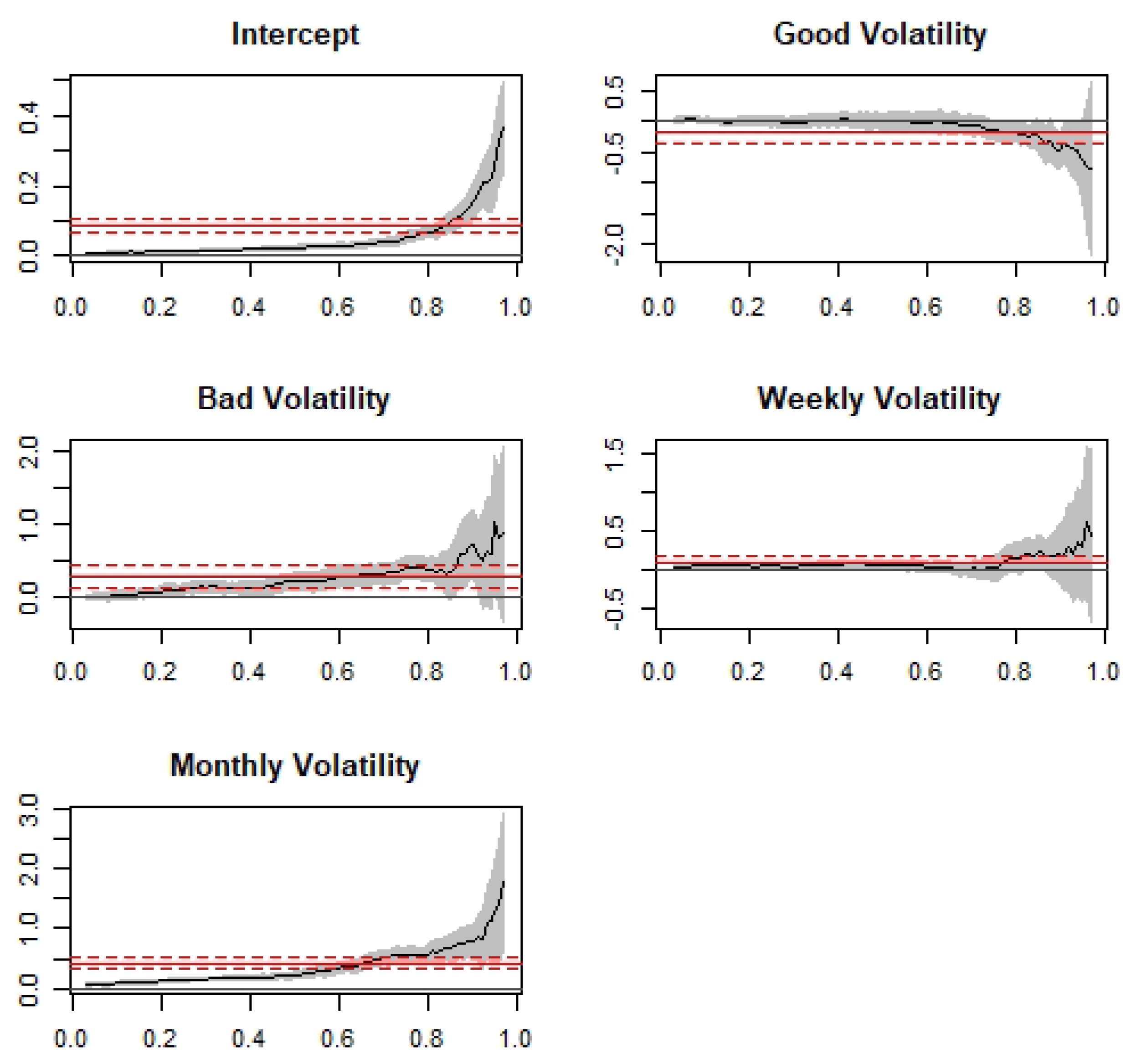
Figure 4.
Good and Bad Volatility for (a) h = 1 and (b) h = 7 forecast horizons.
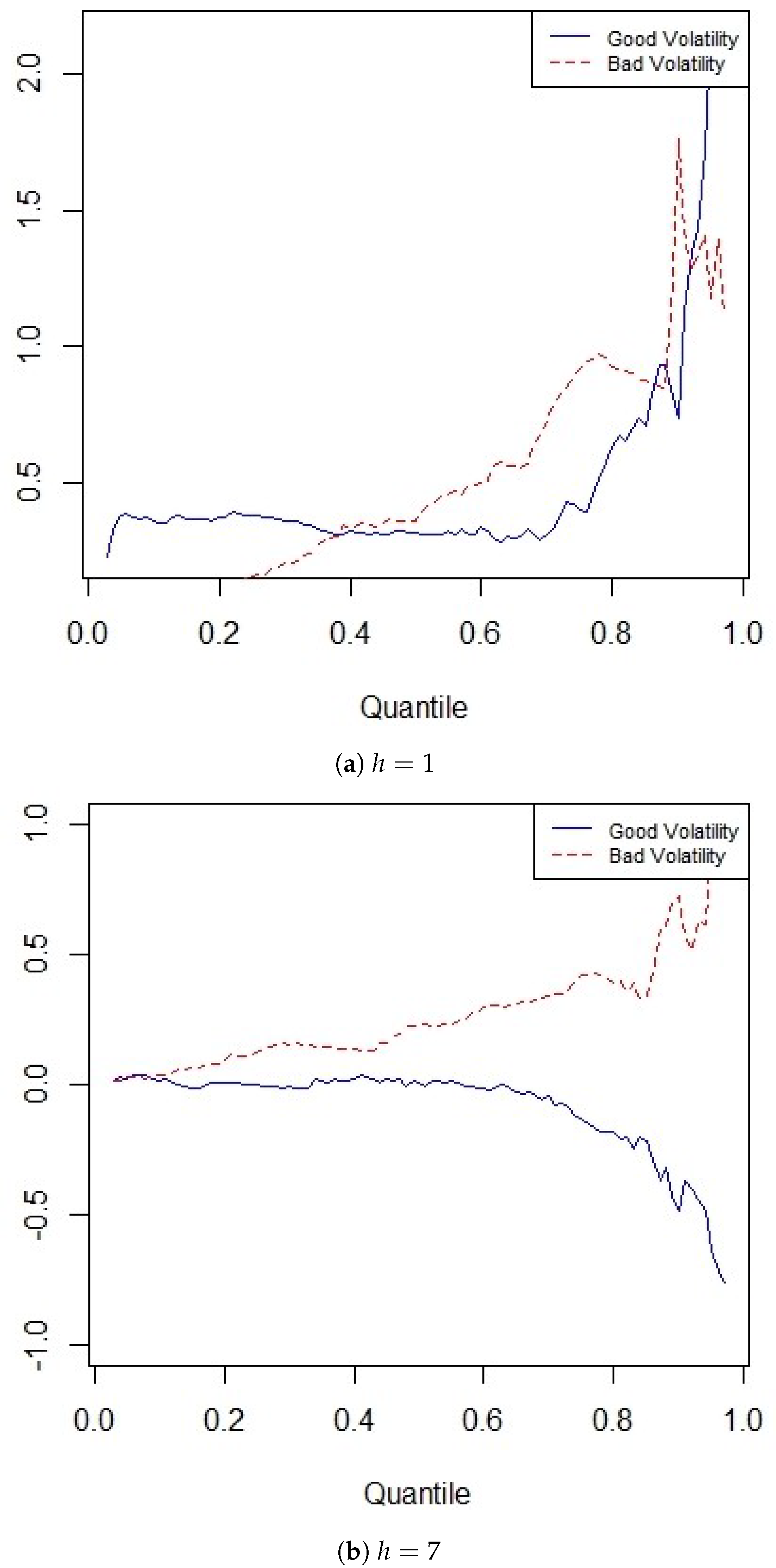
Figure 5.
Model 4: HAR-RV-QR results—1-day ahead.
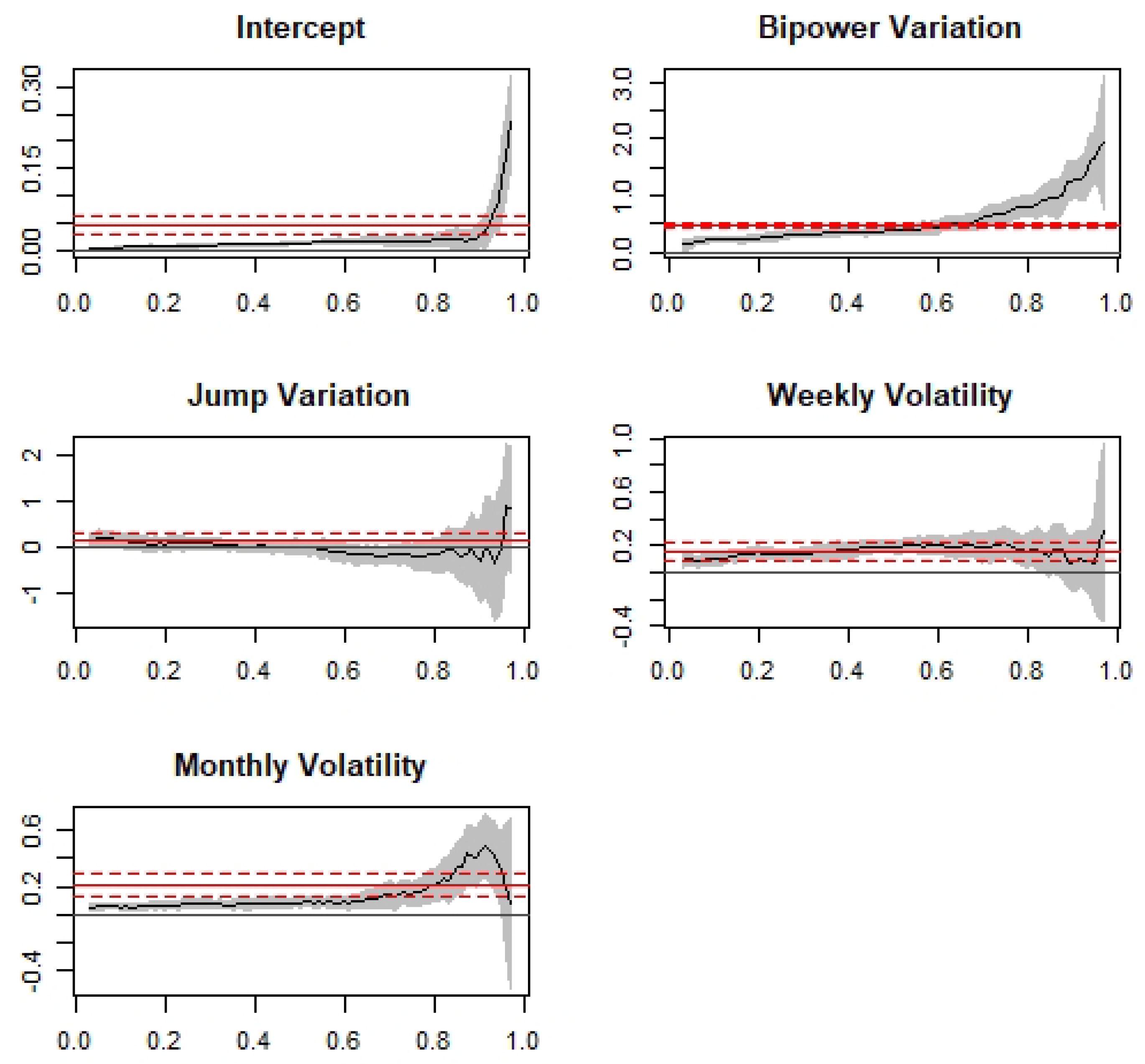
Figure 6.
Model 4: HAR-RV-QR results—7-day ahead.
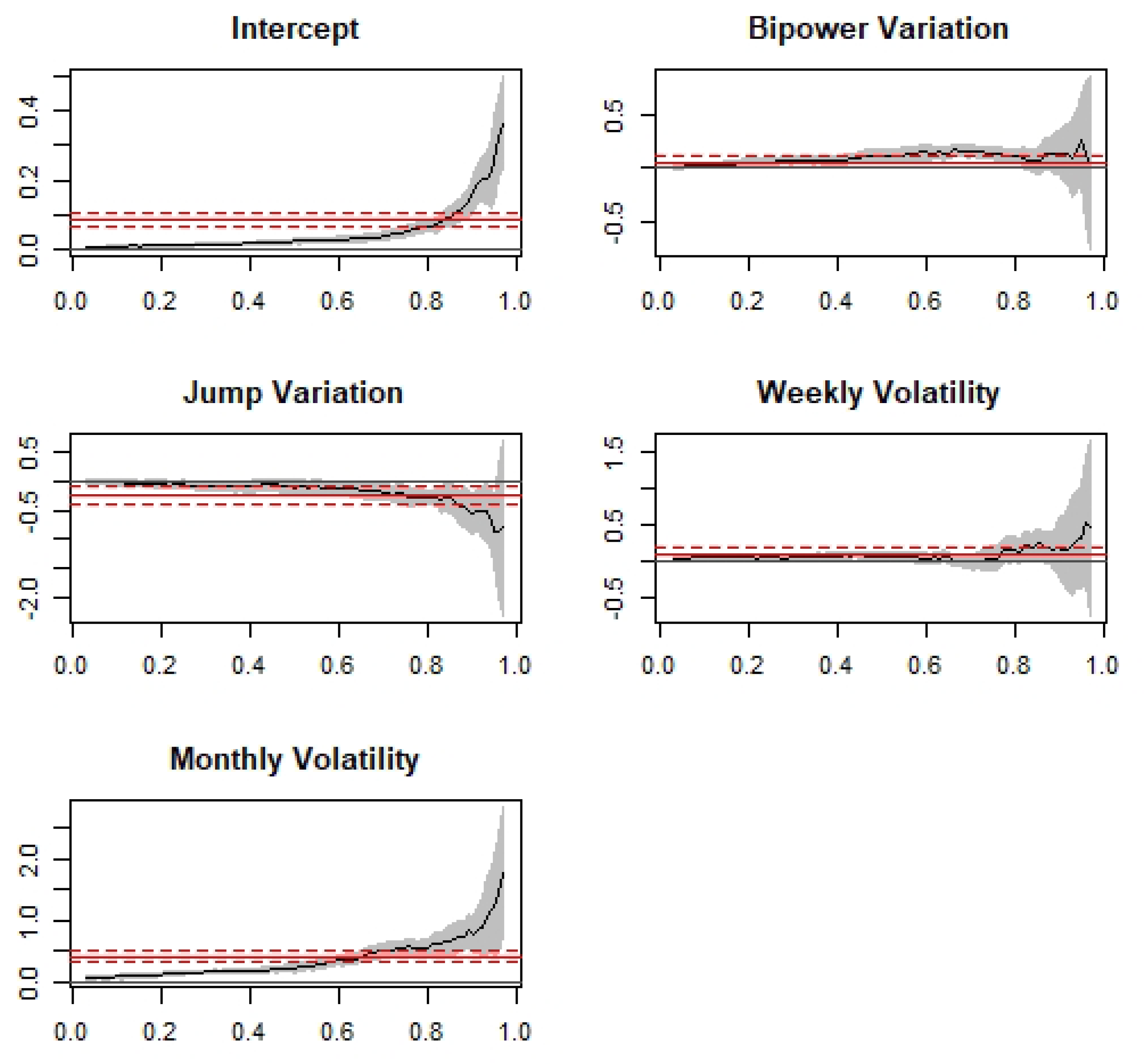
Figure 7.
Model 5: HAR-RV-QR results—1-day ahead.

Figure 8.
Model 5: HAR-RV-QR results—7-day ahead.
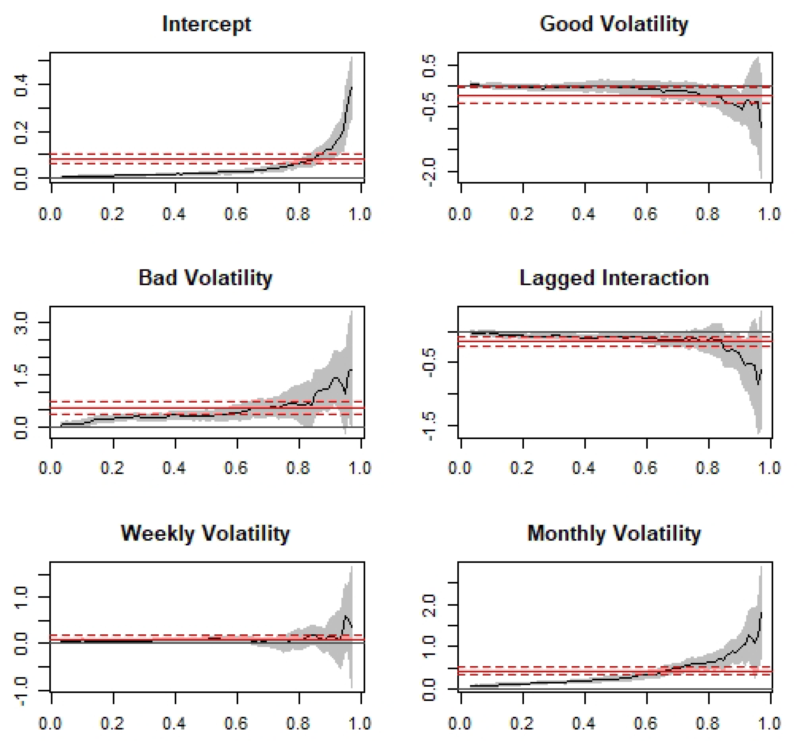
Figure 9.
Predictive power and volatility asymmetry over range of forecast horizons based on Model 2.
Figure 9.
Predictive power and volatility asymmetry over range of forecast horizons based on Model 2.

Table 1.
Summary statistics.
| RV | RS | RS | BV | J | |
|---|---|---|---|---|---|
| Minimum | 0.003 | 0.001 | 0.002 | 0.003 | −4.205 |
| Q | 0.022 | 0.010 | 0.011 | 0.020 | −0.109 |
| Median | 0.097 | 0.045 | 0.048 | 0.085 | −0.001 |
| Mean | 0.225 | 0.106 | 0.119 | 0.204 | −0.012 |
| Q | 0.754 | 0.364 | 0.393 | 0.703 | 0.060 |
| Maximum | 11.360 | 3.578 | 7.782 | 8.452 | 1.104 |
| Correlation Matrix | |||||
| RV | 1.000 | ||||
| RS | 0.960 | 1.000 | |||
| RS | 0.979 | 0.883 | 1.000 | ||
| BV | 0.987 | 0.962 | 0.955 | 1.000 | |
| J | −0.570 | −0.318 | −0.725 | −0.518 | 1.000 |
Q. and Q. are the fifth and ninety-fifth quantiles, respectively. The correlation matrix is significant at the 1% level.
Table 2.
HAR-RV estimation results—1-day ahead.
| Dependent Variable: | |||||
|---|---|---|---|---|---|
| Model 1 | Model 2 | Model 3 | Model 4 | Model 5 | |
| (1) | (2) | (3) | (4) | (5) | |
| 0.040 *** | 0.041 *** | 0.044 *** | 0.044 *** | 0.039 *** | |
| (0.011) | (0.011) | (0.011) | (0.011) | (0.011) | |
| 0.417 *** | |||||
| (0.082) | |||||
| 0.173 *** | 0.162 *** | 0.164 ** | 0.157 ** | 0.158 *** | |
| (0.063) | (0.054) | (0.065) | (0.060) | (0.053) | |
| 0.211 *** | 0.205 ** | 0.209 *** | 0.204 ** | 0.210 *** | |
| (0.081) | (0.080) | (0.079) | (0.077) | (0.081) | |
| 0.239 | 0.345 | ||||
| (0.291) | (0.310) | ||||
| 0.642 ** | 0.625 ** | ||||
| (0.286) | (0.278) | ||||
| 0.450 *** | 0.469 *** | ||||
| (0.092) | (0.084) | ||||
| 0.165 | |||||
| (0.261) | |||||
| −0.073 | |||||
| (0.108) | |||||
| R | 0.321 | 0.323 | 0.327 | 0.328 | 0.324 |
Notes: Newey–West standard errors in parentheses. * p < 0.1; ** p < 0.05; *** p < 0.01.
Table 3.
HAR-RV estimation results - 7-day ahead.
| Dependent Variable: | |||||
|---|---|---|---|---|---|
| Model 1 | Model 2 | Model 3 | Model 4 | Model 5 | |
| (1) | (2) | (3) | (4) | (5) | |
| 0.086 *** | 0.085 *** | 0.086 *** | 0.085 *** | 0.081 *** | |
| (0.022) | (0.022) | (0.022) | (0.022) | (0.022) | |
| 0.081 ** | |||||
| (0.038) | |||||
| 0.084 | 0.097 | 0.085 | 0.096 | 0.088 | |
| (0.095) | (0.098) | (0.095) | (0.096) | (0.094) | |
| 0.096 *** | 0.097 *** | 0.096 *** | 0.097 *** | 0.428 *** | |
| (0.032) | (0.033) | (0.032) | (0.032) | (0.141) | |
| 0.287 *** | 0.512 *** | ||||
| (0.093) | (0.124) | ||||
| −0.179 | −0.215 * | ||||
| (0.112) | (0.111) | ||||
| 0.085 ** | 0.058 | ||||
| (0.041) | (0.042) | ||||
| −0.237 *** | |||||
| (0.092) | |||||
| −0.156 *** | |||||
| (0.056) | |||||
| R | 0.098 | 0.100 | 0.097 | 0.100 | 0.106 |
Notes: Newey–West standard errors in parentheses. * p < 0.1; ** p < 0.05; *** p < 0.01.
Publisher’s Note: MDPI stays neutral with regard to jurisdictional claims in published maps and institutional affiliations. |
© 2020 by the authors. Licensee MDPI, Basel, Switzerland. This article is an open access article distributed under the terms and conditions of the Creative Commons Attribution (CC BY) license (http://creativecommons.org/licenses/by/4.0/).
Share and Cite
MDPI and ACS Style
Jha, K.K.; Baur, D.G. Regime-Dependent Good and Bad Volatility of Bitcoin. J. Risk Financial Manag. 2020, 13, 312. https://doi.org/10.3390/jrfm13120312
AMA Style
Jha KK, Baur DG. Regime-Dependent Good and Bad Volatility of Bitcoin. Journal of Risk and Financial Management. 2020; 13(12):312. https://doi.org/10.3390/jrfm13120312
Chicago/Turabian StyleJha, Kislay Kumar, and Dirk G. Baur. 2020. "Regime-Dependent Good and Bad Volatility of Bitcoin" Journal of Risk and Financial Management 13, no. 12: 312. https://doi.org/10.3390/jrfm13120312