Price Discovery of a Speculative Asset: Evidence from a Bitcoin Exchange


1
Department of Economics and Kenan-Flagler Business School, University of North Carolina, Chapel Hill, NC 27599, USA
2
Smeal College of Business, Pennsylvania State University, University Park, PA 16802, USA
*
Author to whom correspondence should be addressed.
J. Risk Financial Manag. 2019, 12(4), 164; https://doi.org/10.3390/jrfm12040164
Submission received: 28 September 2019
/
Revised: 19 October 2019
/
Accepted: 19 October 2019
/
Published: 25 October 2019
(This article belongs to the Section Financial Markets)
Abstract
:We examine price discovery and liquidity provision in the secondary market for bitcoin—an asset with a high level of speculative trading. Based on BTC-e’s full limit order book over the 2013–2014 period, we find that order informativeness increases with order aggressiveness within the first 10 tiers, but that this pattern reverses in outer tiers. In a high volatility environment, aggressive orders seem to be more attractive to informed agents, but market liquidity migrates outward in response to the information asymmetry. We also find support to the Markovian learning assumption often made in theoretical models of limit order markets.
Keywords:
Bitcoin; cryptocurrency; price discovery; liquidity; price impact; limit order book market; adverse selection; learningJEL Classification:
G10; G12; G14; G19Bitcoin is currently the most prominent cryptocurrency with a market capitalization of approximately $116 billion (as of 26 August 2018). It was created in 2009 by Satoshi Nakamoto (whose identity remains unknown) with the purpose of having “a system for electronic transactions without relying on trust”. However, the nascent literature on bitcoin seems to find converging evidence that people use bitcoin and other cryptocurrencies more as a speculative asset rather than as a medium of exchange (see, e.g., Baur and Dimpfl 2018; Baur et al. 2017; Cermak 2017; Glaser et al. 2014). Notwithstanding, Dimpfl (2017) finds that the adverse selection component of the spread in bitcoin trading is high. This raises an intriguing question about what constitutes private information in the bitcoin market and whether the price discovery process here differs from that of other asset classes.
For equities and fixed income assets, we have the notion of a fundamental price process. What about bitcoin? Reasonable arguments have been put forward questioning the intrinsic value of the cryptocurrency—even claiming it features a purely speculative price bubble process.1 Yet, there is information that should affect the price of bitcoin. For example, the hacking of Mt Gox clearly impacted the notion that bitcoin is immune to cyber attacks.2 Likewise, the ban of bitcoin in countries such as China and South Korea (major hubs for bitcoin mining and trading activities) should matter as well, because it affects the future value of bitcoin as a borderless medium of exchange. How does such information get impounded in the price process of bitcoin? The answer to this question ultimately boils down to how informed agents trade in this market.
The purpose of our paper is to shed light on the microstructure of one of the major bitcoin exchanges—BTC-e. Based on a rich dataset offering a full view of BTC-e’s limit order book across 150 price levels on each side of the market at the sub-second frequency, we are able to measure the extent to which information shows up at the various layers in the book (in addition to trades). The data also allows us to see how liquidity is shifting across the book and to test important implications of adverse selection on market liquidity, differentiating various theories of limit order book markets. With over nearly ten months of trading from 7 December 2013 to 24 September 2014, we are able to characterize the intraday behavior and time series variation of volume, volatility, and liquidity on this important bitcoin exchange.3
Our empirical analysis is based on the Ricco et al. (2018) model of a dynamic limit order market with asymmetric information and non-Markovian learning (that is, traders condition their trading and quoting decision on not only the current state of the limit order book but also the history leading to the current state). The bitcoin market is a great laboratory to test this model given the high level of adverse selection as documented by Dimpfl (2017). In addition, the non-Markovian learning feature of the model appears fitting for the bitcoin market, especially when fundamental information is not present or multiple price equilibria may occur (see Sockin and Xiong 2018 for further discussion). That leaves trade and order history being even more important as the possible source for information extraction. Based on this model, we develop and test three main hypotheses.
The first hypothesis explores the link between orders’ informativeness and aggressiveness, which can then shed light on order strategies pursued by informed traders in this market. Traditional microstructure theories such as Kyle (1985) assume that informed traders exploit their information advantage through market orders—the most aggressive type of orders—, while recent work such as O’Hara (2015) argue that informed traders might prefer to hide information in various layers of the limit order book (i.e., less aggressive orders). The Ricco et al. (2018) model suggests that the relationship between order informativeness and aggressiveness is more nuanced: it depends on the size of the information shock. For large information shocks, informed traders are more likely to trade and quote more aggressively to realize the value of the information quickly. On the other hand, the value of small information shocks might not be sufficient to offset the cost of crossing the spread, thereby inducing them to use less aggressive orders for price improvement.
We find that on average, there is a positive relationship between order informativeness and aggressiveness up to the 10th level in the book. Beyond this level, however, the information content of an order is greater the deeper it is in the book, a finding that would be consistent with the action of informed traders with noisy signals. We then test how this relationship changes in large value shock and small value shock environments. Our hypothesis states that in the former, the relationship between informativeness and aggressiveness becomes more positive (or less negative for the outer region of the book with negative relationship). The parallel hypothesis for low value shock environment is that the positive (negative) relationship between informativeness and aggressiveness lessens (strengthens) as informed traders resort to less aggressive orders for the price improvement.
Our results support these hypotheses. Limit orders at or near the market (most aggressive limit orders) become significantly more informative, whereas limit orders farther away from the market (less aggressive limit orders) become significantly less informative, on days with large information shocks. In a low volatility environment, however, the most aggressive order types, namely marketable orders and inside limit orders, become less informative while the less aggressive limit orders residing between level 6 through 50 become significantly more informative. Our findings support the idea that the size of the information shock matters for informed traders’ order strategies.
The second hypothesis is concerned with how adverse selection affects market liquidity. If the first hypothesis uncovers the strategies of the informed traders, market liquidity as examined in the second hypothesis is the outcome of the interaction of informed and uninformed traders, given that this is a limit order market in which liquidity is supplied by the participants themselves. How adverse selection influences this outcome is an empirical question. Ricco et al. (2018) differentiate between whether adverse selection is due to an increased fraction of informed traders (holding the shock size fixed) or the occurrence of a large shock. In the former case, the increased fraction of informed traders does not change the informed traders’ strategies but drive uninformed liquidity away from the market, resulting in a liquidity reduction. The latter is more complex, because a large value shock can induce informed traders to trade and quote aggressively, namely an inward migration of informed liquidity. At the same time, due to increased pick-off risk, uninformed liquidity is expected to move outward. Accordingly, the net outcome could be either an increase or decrease in market liquidity.
To test the second hypothesis, we use the measure developed by Cont et al. (2014) to proxy for the amount of adverse selection at the hourly frequency. We use the slope of the limit order book to capture market liquidity along both the quantity and price dimensions. Most importantly, the slope can capture the migration of liquidity toward or away from the market and allows us to test the theory discussed above as close as possible. This is a novel feature of our exercise, which is possible only with the full limit order book data used in this paper. We find that in a normal environment, increased adverse selection is associated with a flatter slope, as limit orders migrate to more conservative prices. In a large value shock environment, the slope becomes even flatter, suggesting a significant reduction in liquidity. In contrast, the limit order book slope steepens significantly in low value shock environment, making it easier and less costly to trade. These results contribute empirical evidence to further our understanding of Ricco et al. (2018)’s model.
The third hypothesis directly tests Ricco et al. (2018)’s assumption of non-Markovian learning in financial markets. If price discovery is non-Markovian, lagged market variables should have incremental explanatory power, over and above that of the current state variables. In other words, traders learn from not only the current state of the limit order market, but also the path leading to the current state. Based on predictive regressions of current state variables and their 24-h histories on hourly price impact measure, we find no concrete evidence of the order book history having a significant predictive power over that by the current state variables. One important caveat of this exercise is that we examine only the linear form of dependency, and thus our evidence permits only a qualified conclusion that there is no linear dependency of price discovery on the history of the individual state variable. Our findings do not rule out the possibility that the dependency could be of a non-linear form, or on some combination of the state variables. That said, the lack of evidence for non-Markovian learning in the linear form suggests that the Markovian learning assumption typically adopted in limit order book models might not be unreasonable. This assumption is important because it allows theorist to simplify the state space significantly. Our results here provide some initial empirical support for this assumption in modeling limit order markets. Furthermore, as noted earlier, some bitcoin pricing models suggest that multiple price equilibria may occur, see in particular Sockin and Xiong (2018). In their model, multiple equilibria occur endogeneously and relate to future trading benefits of the cryptocurrency. Although this is one of several theoretical bitcoin pricing models that have been proposed, our empirical analysis suggests that such pricing behavior might potentially be well approximated by a Markovian regime-switching model.
Our study contributes, first and foremost, to the nascent literature on bitcoin in general and the microstructure of secondary market trading in this cryptocurrency in particular. Bitcoin is traded around the clock on many exchanges globally, all of which operate as limit order markets. As in any limit order market, the key question of interest is how informed traders choose their strategies and how the uninformed learn value relevant information from market observables. Even though this question is relatively well researched across many asset markets, bitcoin is an interesting and unique asset in part because the asset pricing theory is still in flux. It is not clear what constitutes fundamental information underlying the intrinsic value of bitcoin. Furthermore, as argued by Zimmerman (2018), bitcoin is extremely volatile and attracts speculative trading due to the unique blockchain structure. Accordingly, it is possible that the price dynamics are sentiment-driven and that traders’ strategies might differ from what we know based on prior theories and empirical work. It is an interesting question whether these unique features of bitcoin could upend the predictions from current theories of limit order markets.
The paper also contributes to the literature on limit order markets. Our paper is based on the full limit order book data, which permits a study of the information content and liquidity across the whole book, not just those pertaining to the top tier or the top few tiers as is commonly done in the literature. With the benefit of observing a more complete state space and action space, the obtained evidence provides a more complete view of order strategies of informed agents and market liquidity. Our evidence therefore can be helpful for the development of theoretical models aimed at capturing more realistically the dynamics of a limit order market, as well as for the interpretation of such models. An additional advantage of using the bitcoin market as an empirical lab for testing limit order market models is that it is relatively free from market frictions (e.g., free entry, no minimum order size or tick size)—a common assumption that usually does not hold in more traditional asset markets.
The paper proceeds as follows. We review the literature on the microstructure of the bitcoin market and derive testable hypotheses in Section 1. We then describe our data and provide summary statistics in Section 2. Section 3 examines the link between order aggressiveness and informativeness in relation to the size of the information shock, providing evidence on order strategies of informed traders. Section 4 analyzes the relationship between adverse selection and market liquidity. In Section 5, we discuss our tests of the non-Markovian learning property. Finally, Section 6 concludes.
1. Related Literature and Testable Hypotheses
Our paper belongs to the small but growing literature that focuses on the microstructure of the secondary market for bitcoin and determinants of bitcoin returns. We review some of the relevant papers in the first subsection. In the second subsection, we state the hypotheses of direct interest that are subsequently tested in our empirical analysis.
1.1. Related Literature
Balcilar et al. (2017) analyze the relationship between trading volume and bitcoin returns and find that volume can predict returns except in bear and bull markets, but cannot predict volatility. Eross et al. (2017) find that volume, bid-ask spread, and volatility all have n-shaped patterns, and conclude that European and North American traders are the main driver of trading activity in this market. Polasik et al. (2015) show that bitcoin returns are driven primarily by its popularity, public sentiments, and the total number of transactions. Dimpfl (2017) finds that the adverse selection component of the spread is high. Caporale and Plastun (2019) examine the day-of-the-week effect in cryptocurrency markets and find no evidence of this anomaly in most crypto currencies except bitcoin, whose returns on Mondays are significantly higher than on other days. They view this finding as evidence against efficiency of the bitcoin market. Detzel et al. (2018) find that bitcoin returns are predictable by the 5- to 100-day moving averages of its prices but largely unpredictable by macroeconomic variables. They explain this finding with an equilibrium model of rational learning in the absence of fundamental cashflow information. Makarov and Schoar (2018) document large and persistent arbitrage opportunities across cryptocurrency exchanges, a result they attribute to capital controls that prevent arbitrage capital from moving freely across borders.
Also related are studies that focus on measuring volatility and understanding the dynamics of jumps in bitcoin prices. Conrad et al. (2018) use the GARCH-MIDAS model to extract the long- and short-term components of bitcoin’s volatility and explore potential macroeconomic determinants of bitcoin’s long-term volatility. Out of the many macroeconomic variables considered, only four have significant effects on bitcoin’s long-term volatility (i.e., U.S. stock market volatility, U.S. volatility risk premium, global economic activity, and bitcoin’s own trading volume). Scaillet et al. (2018) find that jumps occur frequently on Mt. Gox, a major bitcoin exchange before its bankruptcy in March 2014. They show that order flow imbalance and the widening of the bid-ask spread can predict jumps, which in turn have a short-term positive impact on market activity and induce persistent price changes.
With bitcoin being viewed as an asset (albeit a speculative one) and traded on exchanges that operate as limit order markets, its secondary market is similar in many respects to that of other financial instruments. Thus, our study also belongs to the large literature that models and studies price discovery, liquidity provision, and order strategies in limit order markets. The differences between bitcoin and other financial assets, however, can deliver important insights as to the key drivers of market dynamics. We draw upon the theoretical model by Ricco et al. (2018) (henceforth RRS2018) to empirically study the link between information asymmetry and order strategies, which in turn has important implications for the price discovery process. We discuss this model and derive our testable hypotheses in the next subsection.
Finally, it is important to note that alongside the literature on cryptocurrency trading is a more established literature on blockchain technology, smart contracts underlying the working of distributed ledgers, and the organization and economics of mining and verifying transactions (see Malinova and Park 2017 for a thorough discussion of this literature). Pagnotta and Buraschi (2018) develop the first equilibrium model of bitcoin value in a decentralized financial network, based on the interaction of agents’ demand for the censorship-resistance of transfers and the ability to engage in trustless exchanges, with miners’ endogeneous supply of harshing power. Thus, the model provides important insights into what can serve as the “fundamentals” of bitcoin value. Zimmerman (2018) provides a model to explain how the limited blockchain capacity gives rise to the extreme price volatility and the disproportionate extent of speculative trading in bitcoin, linking the “primary market” to important secondary market features of cryptocurrencies. Our paper is on the microstructure of the secondary market where bitcoin is traded, focusing more instead on the interaction of liquidity providers and demanders and how such interaction affects bitcoin returns.
1.2. Testable Hypotheses
The main objective of this paper is to study the extent to which limit order book activities contribute to the dynamics of bitcoin price. Our empirical analysis is built upon RRS2018’s model that extends the framework developed in Kyle (1985) for a limit order market in which informed traders can exploit their information advantage through either market or limit orders at varying prices. Featured in their model are informed traders who have perfect information on the value shock that is eventually realized in the final trading round, and uninformed traders who use Bayes’ rule and observable market dynamics over time to learn about the value shock. RRS2018 characterize the optimal order-submission strategy of informed and uninformed traders at each point in time, conditioning on the path of the limit order book up to that point. As in other theories of limit order markets, the key trade-off is between price improvement and trading immediacy. Whether the information asymmetry arises from a large value shock or a greater fraction of informed traders can result in different effects of adverse selection on market liquidity and price discovery. The model provides three important empirical predictions.
First, when information asymmetry arises from a large value shock, informed traders are more likely to increase their trading and quoting activities at or near the market, because those orders have a higher execution probability and the magnitude of the private information is sufficiently large that such executions are profitable. However, this substantially increases the picked-off risk for the uninformed, inducing them to refrain from trading or quoting too close to the market. Accordingly, in this environment, the informativeness of more aggressive orders is higher. On the other hand, in a low volatility environment, the information advantage is too small to outweight the costs of trading or quoting aggressively. Hence, it is more likely that informed traders post orders further out in the book for the price improvement. In an experimental study, Bloomfield et al. (2005) also find that informed traders are more likely to take liquidity when the value shock is large, but switch to providing liquidity when the value shock is small.
If the channel discussed above reflects informed traders’ behavior in this bitcoin market, we expect to find:
Hypothesis 1A.
The information content of limit orders at or near the market increases, while the information content of limit orders at outer tiers decreases, in a high volatility environment.
Hypothesis 1B.
The information content of limit orders at or near the market decreases, while the information content of limit orders at outer tiers increases, in a low volatility environment.
Second, while the prediction on the informativeness of market and limit orders at the inside and outside tiers is unambiguous, the effect of adverse selection on market liquidity is more nuanced. Theoretical work in this area provide different predictions, depending on how adverse selection is defined and which measure of liquidity is used. For example, in Rosu (2019), adverse selection is defined by the fraction of informed traders in the market; the higher this fraction, the faster is information incorporated in prices and thus the higher the market liquidity as measured by a narrower bid-ask spread. In Goettler et al. (2009), adverse selection arises due to innovations in the asset’s fundamentals. It reduces liquidity at the best quote but increases liquidity behind the best quote, because informed agents use marketable orders while other agents submit more conservative limit orders.
The RRS2018 model considers both types of adverse selection: one driven by the value shock size and the other by the fraction of informed traders in the market. However, their results are based on numerical analysis and could depend on the specific parameters adopted. They find that when adverse selection increases due to an increase in the fraction of informed traders while holding the value shock size fixed, the liquidity provision strategy of the informed does not change, while uninformed traders reduce their trading and quoting activities near the market in response to the increased level of adverse selection. This situation results in an unambiguous net reduction in liquidity at or near the market, but increased liquidity at more conservative price levels—a result opposite that of Rosu (2019). RRS2018’s numerical results for the case in which adverse section increases due to a large value shock indicate that liquidity at or near the market could improve. This is because informed traders are likely to increase their trading and aggressive limit order activities, thereby raising liquidity provision at more aggressive price levels, which in turn could outweigh the reduction in uninformed liquidity. It remains an empirical question whether the net change is an increase (decrease) in liquidity flowing toward the market, implying a steepening (flattening) of the order book slope. The above discussion gives rise to the second set of hypotheses:
Hypothesis 2A.
Adverse selection due to large value shock can improve liquidity and be associated with a steeper slope of the limit order book.
Hypothesis 2B.
Adverse selection due to increased fraction of informed traders reduces liquidity, i.e., is associated with a flatter slope of the limit order book.
Finally, the model predicts that order history carries information beyond that conveyed by the current state of the limit order book. This arises because uninformed traders is using Bayesian updating to learn about the value shock. The path that leads the market to its current state therefore has important implications on the price impact of order flow. If so, we expect that lagged limit order book variables have incremental explanatory power on the price impact of order flow after controlling for the most current state of the limit order book. We thus have the third hypothesis:
Hypothesis 3.
Lagged order book variables have significant explanatory power on price impact of order flow over and beyond the most current state of the limit order book.
We focus specifically on testing for the linear form of history dependence, that is, lagged order book variables enter a linear regression linking price impact with current order book state. It is important to note that a failure to reject the null does not invalidate the non-Markovian property of learning as featured in this model. All we can conclude from this test is whether price discovery in this market is linear non-Markovian. It is still plausible that the history dependency takes on some non-linear form, or that the history of the variables considered is not the one that matters. The RRS2018 model is still under development with respect to which types of histories are important. Nevertheless, studying one set of order book variables and one specific form of history dependence is the first important step toward understanding the nature of learning in the market, and provides useful empirical evidence for further theory development.
2. Data
We use data from BTC-e, which is a digital currency trading platform founded in July 2011. It operated as a limit order market in which users can trade with one another via market or limit orders. The platform allowed trading between several cryptocurrencies (bitcoin, litecoin, namecoin, novacoin, peercoin, dash and ethereum) and three fiat currencies (U.S. dollar (USD), Russian ruble and Euro), but in this paper, we focus on the bitcoin–USD pair. The platform charged a flat fee of 0.2% on all transactions. It was seized by the U.S. authorities in July 2017 on international money laundering charges. During its time of operation, BTC-e was one of the largest cryptocurrency exchanges in the world, serving approximately 700,000 users including a large customer base in the U.S.4 BTC-e was operated by a complex web of entities located in Russia, Bulgaria, and elsewhere, but its servers were located in the U.S.
2.1. The Data
The data was collected through direct API access provided by BTC-e to query transaction history and limit order book snapshots.5 Data collection began on 6 December 2013 and ended on 25 September 2014 (we exclude these two end dates from the sample due to incomplete data on the full 24-h day). This period encloses several major events in the cryptocurrency world, most notably the collapse of Mt. Gox in February and March of 2014. Appendix A provides the list of news articles covering important events in the cryptocurrency world in general, and bitcoin in particular.
During the sample period, two computers simultaneously pinged BTC-e’s servers approximately every 0.1 s, took snapshots of the limit order book, and downloaded the most recent 150 transactions. The two computers ran in parallel, so that if one computer was down, the other was still available for the downloading to ensure completeness. We unify these two separate datasets and clean them as follows.
For transaction history data, each trade record has a unique order ID, so it is straightforward to merge the two transaction histories and eliminate duplicates. Transaction history data contain the following variables: transaction date-time stamp (one-second resolution), transaction price, quantity transacted, trade type (“ask” for seller-initiated and “bid” for buyer-initiated trades), and the order number. It is important to note that a large market order, upon arrival, might execute against multiple limit orders, each of which appears as a separate record in the transaction history data and is given an order number. As in the literature, we aggregate multiple records that likely belong to the same market order as one single trade. We identify a sequence of trade records as belonging to a “parent” market order if the following apply: (1) they span at most two consecutive seconds, (2) have the same trade type (i.e., buy or sell), (3) they occur in non-decreasing prices (for buys) or non-increasing prices (for sells), reflecting the fact that as a market order walks deeper into the book, the prices are sequentially worse, (4) their order numbers are sequential and there is no gap between adjacent orders’ numbers (e.g., 12345678L, 12345679L, 12345680L).6 We then aggregate each identified sequence of trade records to the parent order level by summing up the traded quantities and aggregating the prices in two ways: (1) the price of the last trade record in the sequence, and (2) the volume-weighted average price. We refer to aggregated orders as trades and this is the unit of analysis of trading activity in the rest of the paper. As reported later in the paper, the trade size is still very small, which is likely due to traders slicing their large orders into multiple smaller ones to send to the exchange. The data we have do not contain trader IDs to allow for the identification and aggregation to this level.
The merging and cleaning of the two limit order book snapshot datasets is more involved. It is important to ensure the correct time sequencing of snapshots, which is a challenging task because the latency between each downloading computer and BTC-e’s servers can vary and time stamps are only up to the one-second resolution. The data downloading algorithm captures the start time of a request and the time it takes to finish the downloading of a snapshot. Thus, each snapshot in each dataset has a lower and upper time bounds, based on which we can conservatively supplement gaps in one dataset with available snapshots from the other. After this step, we obtain a combined dataset containing snapshots of the limit order book with 150 price levels on each side of the market at an ultra-high frequency.7 We remove duplicate snapshots when there is no change in any of the price nor quantity in the book. We refer to the resulting dataset as the tick-frequency limit order book data.
To see the extent to which the price on BTC-e differs from that on other exchanges, we plot in Figure 1 the evolution of the best mid-quote on BTC-e at the one-minute frequency and the daily closing price collected by CoinMarketCap, a cryptocurrency market tracking company. Except for the earlier part of the sample period, the price on BTC-e aligns quite closely with the general price level in the market. In fact, Brandvold et al. (2015) find that BTC-e, together with Mt. Gox, leads in price discovery in a study of seven bitcoin exchanges that collectively make up 90% of bitcoin trades over the period from April 2013 to February 2014. Dimpfl (2017) also finds that BTC-e is the most liquid market for trading bitcoin in U.S. dollar based on data from November 2016 to January 2017.
2.2. The Microstructure of BTC-e
2.2.1. The Limit Order Book
We plot in Figure 2 the average shape of the limit order book, indicating the percentage of cumulative depth up to the 150th tier. The x-axis shows the distance (in cents) from each price level to the mid-quote. For reference, the plot includes a solid line showing cumulative depth in an equally-distributed book. The distribution is convex on both sides, suggesting that there is relatively more depth available the further out the price level. The plot also reveals the difference in how depth is distributed on the two sides. On the ask side, depth is more concentrated at or near the market than that on the bid side. To supplement this plot, Panel A of Table 1 reports some specific depth statistics at select tiers. These statistics further indicate that depth is quite spread out across the book, totaling about 320 coins across 150 price levels on each side, or averaging slightly above 2 coins per tier. At the inside tier, there are about 4.1 bitcoins on the ask and only 2.6 on the bid.
We report the average cost of immediacy as measured by the relative spread at various price tiers in Panel B of Table 1. The spread at a select tier is computed as the difference between the price at that tier and the best price on the opposite side, standardized by the mid-quote. The inside bid-ask spread averages to 19.5 bps, comparable to the bid-ask spread of a large stock. Adding the flat transaction fee of 20 bps charged by BTC-e, the total transaction cost is at least 40 bps.
We also report the volume-weighted spread, computed as the difference between the depth-weighted average of prices up to a given tier and the best price on the opposite side. The simple spread statistics on the bid side up to the 20th tier are smaller, indicating that these bid orders are placed slightly closer to the market than their ask counterparts. However, taking into account their lower quantities (as shown in Panel A), the volume-weighted spread on the bid side is equal to or greater than that on the ask side. Furthermore, beyond the 50th tier, bid limit orders are placed at a further distance as compared to the corresponding ask limit orders. Taken together, the summary statistics presented here indicate that the cost of immediacy for a bitcoin buyer (who takes the asks) is slightly lower than that for a seller (who hits the bids), i.e., it is easier to immediately buy than sell, especially a large quantity.
We examine the time series variation of depth over the sample period (plot available upon request) and find that ask depth appears to fluctuate more than bid depth. Furthermore, there are several spikes in ask depth not accompanied by similar spikes in bid depth, especially at the top 5 price levels. This indicates that most occasions of significant market imbalances are due to excessive selling pressure on the ask side of the book. Perhaps most interestingly, bid depth often leads ask depth. Granger-causality tests with up to 10 lags on the daily average bid and ask depth at the top five tiers and across the whole book all indicate that depth on the bid side systematically leads depth on the ask side. However, this lead-lag relationship prevails only at the daily frequency and not at intraday frequencies.
2.2.2. Trading Activities and Market Volatility
As reported in Table 2, trades on the BTC-e platform occur frequently with nearly 13,000 trades per 24-h trading day on average, for a total of 5626 coins bought and 5752 coins sold. On average, the total dollar volume transacted each day is roughly $7 million. Buyer-initiated trades generally occur more frequently than seller-initiated trades, but with a slightly smaller trade size: 0.84 versus 0.93 coins per average trade (or in the $500 range in dollar trade size). The median of 0.1 coin and the tail statistics (5th and 95th percentiles) indicate that the trade size distribution is highly skewed to the right. 95% of trades are for 4 coins or less, which can be easily absorbed by limit orders at the top tiers in the book.
We find that trading volume is highly correlated with volatility, as shown in Figure 3. We compute daily realized volatility from 5-min mid-quote returns.8 The sample correlation between volume and volatility is nearly 0.68, and they both exhibit multiple spikes around major events in the cryptocurrency world. December 2013 appears to be the most volatile month in the sample period, and includes the biggest spike of over 500% in volatility. Analysis of news events in December points to China Central Bank’s decision on 5 December 2013 to ban financial institutions from handling bitcoin transactions as the catalyst. The collapse of Mt. Gox in late February 2014, the IRS’s decision to tax bitcoin as property in late March 2014, and the closure of bank accounts of Chinese bitcoin exchanges also see volatility shooting up. Interestingly, volatility does not appear affected by Dell’s and Paypal’s announcements to accept bitcoin. This evidence seems consistent with earlier research that bitcoin is used more as an asset than as a currency. The high level of volatility, averaging to about 63% during the sample period, also supports earlier studies’ conclusion that bitcoin is too volatile to serve as a store of value and medium of exchange.
2.2.3. Intraday Patterns
Even though the market operates continuously 24/7, intraday patterns of key market variables in Figure 4 indicate that the most liquid and active time is between 03:00 and 12:00 ET. After 12:00, depth, trade volume, and volatility all trend down. The bid-ask spread stays narrow for a few more hours and only widens significantly after 18:00 We also check if liquidity exhibits any day-of-week pattern widely documented in U.S. equity markets, by regressing different daily liquidity variables on day-of-week dummies. We find that these dummies are rarely significant, providing little evidence for the day-of-week pattern in either depth or trading volume. There is some mild evidence that the bid-ask spread is narrower mid-week (Tuesday through Thursday).
3. Adverse Selection and Order Strategies
In this section, we measure and analyze the information content of market and limit orders, in order to test the hypothesis that the link between order informativeness and order aggressiveness depends on the size of the value shock. Thus, it is important to identify when there is likely a large value shock, and compare the information content of orders of varying degree of aggressiveness in such an environment with that in a normal environment. To strengthen the analysis, we also test if the reverse is true in a low value shock environment.
3.1. Identification of Large Value Shock Environment
As the first step, we partition the sample period into three subsamples corresponding to large value shock, low value shock, and average value shock environments. We use both realized volatility and the high-low range of the midquote to determine these partitions.9 Specifically, for each day, the high-low range is computed as the difference between the log of the highest and lowest mid-quote of the day, based on the raw snapshot data available at the tick frequency. Essentially, this measure captures the return that can be achieved by an informed trader with perfect information who buys at the lowest price and sells at the highest price. Thus, it is a reasonable proxy for the asset value shock signal.
The use of realized volatility to supplement the high-low range is to ensure that a large high-low range reasonably reflects an environment with a large value shock and not one that is otherwise a tranquil day but for a fleeting price outlier. We compute the daily realized volatility by the square root of the sum of squared log returns based on the midquote sampled every five minutes.10 The large (low) value shock days are those days when both the realized volatility and the high low range are in the top (bottom) quartile of their respective distributions. The average environment is defined as the rest of the days in the sample on which the value shock size is neither too large or too small. This exercise results in 62 days in the large value shock subsample, 58 days in the low value shock subsample, and 172 days in the average value shock subsample.
We verify that the procedure above delivers a reasonable partition of the data by conducting a comprehensive news search of important crypto market events from major news outlets, including Bloomberg, Reuters, and popular cryptocurrency news websites CCN and CoinDesk. We then classify these news articles into three broad categories: cybersecurity threats, regulatory changes, or market acceptance. The table below shows the count of each news type that falls into the high value shock, average value shock, and low value shock subsamples:11
| News Type | High | Average | Low |
| Market Acceptance | 2 | 4 | 1 |
| Regulatory | 14 | 14 | 0 |
| Security/Hack | 15 | 16 | 1 |
| Total days with news | 31 | 34 | 2 |
It is clear that a disproportionately large number of important news are in the high volatility subsample, while there is almost no news on low volatility days. This provides further assurance that the high and low value shock subsamples do indeed reflect the difference in their information environment. It is also important to point out that the major type of news during the sample period relates to hacking incidences that expose the security risk of owning and trading bitcoin. Regulatory actions of various governments also seem relevant, much more so than does market acceptance. News of bitcoin being accepted by retailers as a method of payment (e.g., Overstock, Dell, and eBay) does not occur as frequently, and does not seem to be informationally relevant, as indicated in Figure 3 by the muted response of trading volume and volatility upon such events.
3.2. Information Content of the Limit Order Book
An important task in testing Hypotheses 1A and 1B is measuring the information content of limit orders at different price levels in the book. For this, we use Hasbrouck (1995)’s information shares, similar to Cao et al. (2009). With 150 price levels on each side of the market, it is not econometrically feasible to model their dynamics without some data summarizing and dimension reduction. To keep the exercise manageable, we partition the 150 levels of the order book into six categories: tier 1, tiers 2–5, tiers 6–10, tiers 11–50, tiers 51–100, and tiers 101–150, ranging from the most aggressive limit orders to the least aggressive ones. Together with the trade price series, they are all some noisy representation of the true price of one common asset and thus cannot deviate too much from the common underlying price process. Thus, we model their dynamics with a vector error correction (VEC) model based on which to compute their respective information shares. The information share of a price series reflects its contribution to the variance of the permanent price updates: the higher the information share, the more informative a price series is and the more it contributes to price discovery.
Let , where is the last transaction price, and the remainders are depth-weighted average prices corresponding to tier 1, tiers 2–5, tiers 6–10, tiers 11–50, tiers 51–100, and tiers 101–150 (averaged across both sides and all relevant tiers). The VEC model is:
where is a vector of correction terms, i.e.,
In our implementation, we choose and estimate the model separately for each day using one-minute price data. Due to the high dimensionality of the VEC model (7 price series with 10 lags), estimating information shares at intraday frequencies might compromise the reliability of the estimates. The Hasbrouck (1995)’s information shares rely on two ingredients derived from the model. The first is the permanent impact of the shock vector on all cointegrated prices in the system (i.e., the long-run multipliers based on the moving average representation of the VEC model). The second is the vector of orthogonalized shocks, which we obtain via a Cholesky decomposition of the covariance matrix of the residuals . The information share of price series j is then computed as:
where is the permanent price impact of shock i, and is the element of the lower triangular matrix M such that . Thus, the information share of a given price series is the contribution of its variation to the total variation of the efficient price updates. To address the sensitivity of information shares to variable ordering in the model, we perform the calculation for all possible orderings and then compute the average information shares across all orderings. These are the information share estimates we use throughout the paper.
We plot the 7-day moving averages of our information share estimates in Figure 5, with the legend indicating the average information share for each order category over the entire sample period. It is clear that trades and limit orders posted at the top tier of the book account for the largest portion of the total variation of bitcoin price updates, 31% and 28% on average respectively. The remaining 41% average information shares come from the rest of the limit order book. It is interesting to see that information shares do not monotonically decrease the less aggressive the limit orders: they decrease through the 10th level but then increase the further away the limit orders. This is surprising and contrasts with the common belief that information content increases with order aggressiveness. Earlier research into the information content of limit order books, such as Cao et al. (2009), does not go this far into the limit order book. Therefore, it is not clear if we would have seen the same pattern had we examined equity market limit order books beyond the 10th tier, or if this is a peculiar feature of the bitcoin market in which the extreme volatility might increase the probability of execution for further-away orders, thereby inducing informed traders to post more of such orders. This is similar to out-of-the-money options having a greater chance of moving in-the-money the higher the volatility, which can be attractive to informed traders.
3.3. Order Aggressiveness and Information Content
The RRS2018 model predicts that informed traders increase their trading and quoting at the most aggressive price levels when the value shock is sufficiently large. In contrast, in low value shock environment (i.e., the value of the private information is small), it might not be profitable for them to trade and quote aggressively, and hence orders closer to the market might become less informative.
Panels A1–A3 of Table 3 show the average information share of trades and limit orders at varying degree of aggressiveness by the three information environments. Consistent with Figure 5, we observe that trades carry the most information regardless of the information environment, alone accounting for nearly one third of the total variation in price updates. We continue to observe that very little information is conveyed by limit orders at tiers 6–10 (less than 3%). It seems that informed traders either trade or quote very aggressively, or submit orders away from the market.
We then perform a difference-in-mean t-test by comparing, for each order aggressiveness category, the information share in a large (low) value shock environment with that in an average volatility environment. Panels B1 and B2 contain the results of these tests, and they both provide strong support for RRS2018’s model. That is, when the value shock is large, informed traders are more likely to trade and quote aggressively to exploit their information, because the value of the information is more than offset the cost of trading or quoting aggressively. Panel B1 shows that aggressive limit orders (i.e., those placed in the top 10 tiers in the book) become statistically more informative than they normally would in an average volatility environment, whereas limit orders posted beyond the 10th tier become statistically less informative. The evidence provided in Panel B2 for the low value shock environment reveals the opposite, which is that less aggressive orders are statistically more informative, lending further support to the theory that informed traders in such an environment choose to use limit orders deeper in the book, as trading and quoting aggressively is not profitable when the value shock is small.
4. Adverse Selection and Liquidity Provision
We next investigate how adverse selection affects market liquidity through its impact on order strategies of informed and uninformed traders. This exercise helps demonstrate that whether adverse selection hurts market liquidity depends on the nature of the information asymmetry. For this, we first discuss how we construct the measure of adverse selection at an hourly frequency, and the measure that summarizes the state of liquidity supply. Next, we present and discuss our findings.
4.1. Measuring Adverse Selection
Central to our empirical analysis is a measure of the degree of adverse selection in the market. Previous studies traditionally measure adverse selection by the price impact of trades, which reflects the common assumption underlying many traditional microstructure theories that informed traders use market orders to exploit their information advantage. O’Hara (2015) argues that this assumption is increasingly detached from the reality of trading in today’s high frequency trading world. Recent work has argued that informed traders can also utilize limit orders to exploit their information advantage (for theoretical work, see, e.g., Boulatov and George 2013; Ricco et al. 2018; and references therein; for empirical evidence, see, e.g., Fleming et al. 2018; Brogaard et al. 2018; Cont et al. 2014, among others.) As Cont et al. (2014) (CKS2014) argue, trades are not sufficient to capture price movements given the sheer amount of limit order book events between any two trades. Our earlier findings on the information composition of trade and limit order activities also confirm that trades, while accounting for the largest share of price discovery, account for only 30%. The rest of price discovery is due to movements in the limit orders. Accordingly, price impact of limit order book events, and not just trades, is a better measure of adverse selection in a limit order market. Following CKS2014, we estimate this price impact measure by the following regression model:
where is the change in the mid-quote over the sub-interval k of interval i, and is the order flow imbalance that aggregates limit order submissions, cancellations, and executions at the inside tier over the same sub-interval. Estimating Equation (2) separately for each interval i, we obtain the interval’s price impact estimate . To ensure that there are sufficient observations within each interval to reliably estimate , we choose the interval frequency to be hourly (i.e., ), and the sub-interval sampling frequency to be one-minute (i.e., ). To compute , we accumulate changes at the top of the book over the sub-interval k using the raw snapshot data available at the tick frequency. The net order flow between ticks and t is
where and are the price and quantity of coins available at the best bid (similarly defined for the best ask). If price does not change, then the order flow to the bid side is . If there is an improvement in the best bid (i.e., ), the order flow to the bid side equals the size of the new price-improving orders. If there is a cancellation or trade execution that completely wipes out the previous tick’s first tier and pushes the second tier forward (i.e., ), the order flow is decreased by the quantity of the first tier at the previous tick. The same logic applies to the ask side. The net order flow from one tick to the next is therefore the difference between the order flow to the bid (in the first parentheses) and that to the ask (in the second parentheses). We aggregate this net order flow to the sub-interval k level, i.e., .
Panel A of Figure 6 provides summary statistics of . It is reassuring that the estimate is correctly positive 95% of the time (i.e., excess buying pressure results in price increases and vice versa). The distribution is right-skewed indicating the presence of extremely large values, with a mean of 2.4 and a median of 1.65.
4.2. Measuring Liquidity Provision
Given the high dimensionality of the limit order book, the slope of the bid and ask schedules is a useful measure of how willing liquidity providers supply their bids/offers to fulfill trading demand by more impatient traders. Næs and Skjeltorp (2006) examine the slope and show that it is indeed very important for the trading and volatility relationship. Næs and Skjeltorp (2006) first measure the slope locally at each price level by the ratio of the increase in depth over the increase in price, then average across all price levels and the two sides of the book to obtain an average slope measure. Our full limit order book data allows us to estimate the slope compactly with the following regression:
where is the percentage of cumulative depth at tier () as of the end of interval i and is the distance between the price at tier and the best bid-ask midpoint . We estimate the slope separately for the bid and the ask side and for each interval i, and denote them by and .
Because we standardize cumulative depths by the total depth across all 150 tiers, is always 100%. Therefore, the slope measure depends merely on how wide the 150-tier pricing grid is (the intercept already takes care of ). Accordingly, our slope measure captures the tightness of prices in the book. A steeper slope indicates that limit orders are priced closer to the market. Figure 7 illustrates how the slope captures the liquidity distribution in the book. Another way of interpreting the slope is that it measures the elasticity of depth with respect to price. A steeper slope implies that for one unit increase in price, there is a greater increase in the quantity bid or offered, implying a greater willingness of liquidity providers to facilitate trading demand on each side of the market.
We plot the histogram of the slope estimates in Panels B and C of Figure 6. Both slopes are strictly positive, reflecting that liquidity supply is greater the better the price for the liquidity providers. With zero being the lower limit, both distributions have long right tails. The ask slope is steeper than the bid slope, as indicated by both the mean and the median, and has more variability. This suggests a greater but also more volatile willingness to provide liquidity on the ask side.
4.3. Does Adverse Selection Worsen Market Liquidity?
To test hypothesis 2A and 2B, we run the following regression:
where is the slope of the order book at the end of hourly interval i, is the measure of adverse selection for interval i, is an indicator for days with a large value shock, is an indicator for days with a low value shock, and are control variables. Included in are: (1) the slope on the opposite side (to see if liquidity provision on one side interacts with that on the other), (2) the total number of coins bid and offered in the book (to control for the absolute amount of liquidity available at any given point in time), (3) the fraction of depth residing at the top (to control for the possibility that a flat slope can also reflects the front-loading of depth at the top tier), (4) the current level of trading activity (to assess if trading demand plays a role in shaping liquidity provision), and (5) the prevailing volatility in the market (as volatility is well documented to affect liquidity). Depth, trading volume, and trade count are log-transformed. We also estimate a specification that includes hourly dummies to account for any diurnal effects on the order book shape and liquidity provision. We use robust regression methodology to minimize the potential impact of outliers on the results. We report the results in Table 4. The key estimates—, , and —appear on the first three rows.
Robust across side and specifications is a significantly negative —the coefficient for —indicating that increased adverse selection is associated with a flatter order book slope. Moreover, the significantly negative coefficient on indicates that the already negative association of adverse selection and liquidity becomes even stronger on days when large value shocks are likely present. On the other hand, in a low value shock environment, the order book steepens significantly as shown by the significantly positive estimates of , suggesting a greater liquidity supply. Unreported tests indicate that the sum of and is significantly positive, that is, on low volatility days, adverse selection is positively associated with liquidity provision.
The flattening of the order book in the high value shock environment, compared with the steepening of the order book in the low value shock environment, indicates that it is the value shock size that matters for both informed and uninformed traders. In an environment where adverse selection is due to a large value shock, informed traders are likely to trade and quote more aggressively, resulting in informed liquidity moving toward the inside tier. However, worried about the risk of being picked off, uninformed traders’ liquidity moves away from the market. Our findings are consistent with the outward migration of uninformed liquidity outweighing the inward migration of informed liquidity, resulting in the flattening of the order book slope.
Within each information environment, the variation of adverse selection is likely due to changes in the fraction of informed traders. However, the evidence only supports hypothesis 2B (that adverse selection due to increased fraction of informed traders worsens liquidity) in the high value shock environment. In such an environment, the increased fraction of informed traders heightens the picked-off risk and contributes to drive uninformed liquidity away from the market. The opposite evidence obtained for the low value shock environment does not support RRS2018’s prediction, but is instead consistent with Rosu (2019)’s intuition that the increased fraction of informed traders facilitates better learning by uninformed traders, thereby improving liquidity.
5. Is Price Discovery History-Dependent?
Another important implication of RRS2018’s model is the non-Markovian property of information learning in a limit order market. It implies that the price impact of order flow depends not only on the current state of the limit order book, but also on the history of past order actions leading up to the current state. Given that the history space is large, it would be desirable to have some theoretical guidance as to what types of histories matter most for price discovery. The theory is still under development in this regard. Here, we rely on the data to tell us which part of the history that is important.
One important caveat is that, order history can enter the price discovery process in some unknown form. Our empirical analysis below looks specifically for linear effects, recognizing that the lack of evidence for the non-Markovian property in the linear sense does not imply that price discovery is not non-Markovian. It could still well be, just not in a linear form. Alternatively, the specific elements in the history space we consider are not the ones that matter. Nevertheless, it is still a very useful exercise to at least know that certain elements and certain forms do not work. This would be especially helpful for the development of theories with respect to the non-Markovian learning implication.
We test for the linear non-Markovian property by regressing the hourly price impact—the measure of price discovery—on a set of variables that capture the current state of the limit order book. These are: (a) the total depth on each side, (b) the concentration of depth at the top tier on each side, (c) the concentration of depth at the top 5 tiers on each side, (d) the slope of the order book on each side, (e) the level of buying and selling activity in the market, and (f) the prevailing short-term volatility. Order book variables (a, b, c, d) are measured at the beginning of each interval. Trading and volatility variables (e, f) are measured over each interval, similar to the way the dependent variable is measured. We then add the history of each of these variables, one by one, to the regression to determine if the lagged values of the chosen variable have any incremental explanatory power over the price discovery measure. We allow for a 24-h history in these variables, that is, we include 24 lags of each covariate. Let be the vector collecting all of the above 11 explanatory variables for the hourly interval i, while denotes the individual explanatory variable j. We run the following regression for each explanatory variable j:
Panel A of Table 5 shows the baseline regression results that include only the explanatory variables that capture the current state of the limit order book. The regression results are consistent with intuition: (1) price impact is lower when trading is more active (regardless of the side), (2) price impact is higher when the market is more volatile, (3) greater ask depth (indicating increased selling pressure) dampens price impact while greater bid depth (indicating increased buying pressure) increases it, and (4) a greater concentration of depth at the top 5 tiers reduces price impact.
It is interesting to note that the concentration of depth at the top tier does not explain price impact, nor does the slope. It seems that market participants care only about the total amount of depth in the book and how much of that depth resides at the top 5 tiers. We also include hourly dummies to control for the potential diurnal pattern of price discovery, but find that these dummies have little explanatory power, and that the coefficients of order book variables remain robust to the inclusion of the hourly dummies. Thus, for regressions that include lagged explanatory variables, we use the baseline model without the hourly dummies.
Panel B of Table 5 documents the incremental explanatory power of each covariate’s 24-h history, as indicated by the number of lags with a significant coefficient and the adjusted of the regression. These lags are rarely significant. At the 1% significance level, the history of most order book variables studied here is completely insignificant (except the total bid depth and the realize volatility, each of which has only 1 significant lag out of the 24-h history). Even at the 10% significance level, the number of significant lags for most variables is very small, at most 4 out of 24. In addition, the inclusion of the lags reduces the adjusted , as opposed to increasing it. Overall, Panel B shows little support for the linear history-dependence of price discovery.
6. Conclusions
Our paper provides an in-depth analysis of the information content and liquidity of the limit order book on a major bitcoin trading platform. We find several important results that contribute to both the growing literature on bitcoin trading and the literature on limit order book modeling.
First, trades and limit orders at the best bid and ask are most informative. The information content then decreases the more conservative the price up to the 10th best level, and mildly increases for orders posted at far-away tiers. In a high value shock environment, aggressive orders become more informative, suggesting the increased use of such orders by informed traders. On the other hand, in a low value shock environment, the informativeness of market orders and best limit orders is reduced while that of mid-book orders increases. Second, we find that the information shock size matters for market liquidity. When asset volatility is high, adverse selection worsens liquidity, in contrast to the improved liquidity in the low volatility environment. Overall, the complex liquidity and volatility dynamics reported in our paper provide further justification for the skepticism on the part of monetary policy authorities towards the broad use of cryptocurrencies.
Lastly, we do not find concrete evidence to support the linear dependency of price discovery on the history of individual state variables. This result indicates that the Markovian learning assumption typically adopted in limit order market models might not be unreasonable after all. Future research can shed further light on this important assumption by employing non-linear models of dynamic limit order books (see, e.g., Nguyen et al. 2019). Such research will be valuable in enhancing our understanding of the complex dynamics of price discovery in limit order book markets.
Author Contributions
The authors contributed equally to this work.
Funding
This research received no external funding.
Acknowledgments
We are grateful to Jacob Sagi for providing the data used in this paper. We thank Ekkehart Boehmer, Pab Jotikasthira, Stefan Lewellen, Duane Seppi, Kumar Venkataraman, Mao Ye, and participants at the 2018 NBER Big Data and High Performance Computing for Financial Economics workshop, Penn State University, Southern Methodist University, UC Louvain, and 2018 SFS Cavalcade Asia-Pacific for helpful comments. We also thank Joseph Pate for excellent research assistance. This paper was previously titled “Bitcoin Price Discovery”.
Conflicts of Interest
The authors declare no conflict of interest.
Appendix A. Cryptocurrency News Articles
| Date | Title |
| 5 December 2013 | A Better Translation Of People’s Bank Of China’s First Official Statement On Bitcoin |
| 5 December 2013 | China bans banks from handling Bitcoin trade |
| 6 December 2013 | People’s Bank of China Issues a Regulatory Notice on Bitcoin |
| 7 December 2013 | BTC China now Requires ID Verification from All Users Upon Logging In |
| 7 December 2013 | The UK can Finally Have a Real Bitcoin Exchange |
| 14 December 2013 | Taiwan Bitcoin Exchange |
| 16 December 2013 | Norway Doesn’t Consider Bitcoin a Legitimate Currency |
| 17 December 2013 | People’s Bank of China Further Restricts Bitcoin |
| 19 December 2013 | Chinese Bitcoin Exchange Accepting Deposits |
| 20 December 2013 | Overstock.com Will Start Accepting Bitcoin In 2014 |
| 23 December 2013 | Chinese Bitcoin Ban Driven by Chinese Banking Crisis? |
| 23 December 2013 | New Indonesian Bitcoin Exchange Could Help Spur its Economy |
| 25 December 2013 | HashCows Mining Pool Hacked |
| 26 December 2013 | Online Dogecoin Wallets Hacked |
| 27 December 2013 | Chinese Bitcoin Exchanges Find Workaround To Allow RMB Deposits, Exchange Rate Rallies |
| 28 December 2013 | The US Department of Treasury issues a Bitcoin-Friendly ruling for Miners |
| 30 December 2013 | Bitcoin’s Uncertain Fate in India |
| 6 January 2014 | Indian Exchange Unocoin To Resume Operations |
| 7 January 2014 | Bitstamp is down |
| 7 January 2014 | Taobao.com (China’s Ebay) Bans Bitcoin Payments |
| 9 January 2014 | Ghash.IO official statement on the 51% attack threat |
| 12 January 2014 | Warning: Huobi has closed their personal bank accounts system |
| 13 January 2014 | The Bitcoin Price Falls due to Concerns with China |
| 14 January 2014 | OpenEx Hacked |
| 17 January 2014 | Ebay will allow Bitcoin Trading |
| 20 January 2014 | Finland Decides To Treat Bitcoin As A Commodity |
| 23 January 2014 | Give Me COINS Litecoin Pool Hacked |
| 27 January 2014 | BitInstant CEO and Bitcoin Foundation Vice Chairman Charlie Shrem Arrested in New York |
| 28 January 2014 | The Epic Fall Of Mt. Gox: The Increasingly Illiquid Bitcoin Exchange |
| 28 January 2014 | Central Bank of the Russian Federation Discourages Use of Bitcoin |
| 1 February 2014 | Bitcoin Now Accepted at Every 7-Eleven in Mexico |
| 3 February 2014 | Calm Down Internet, BTC-e is Not About to Be Shutdown |
| 5 February 2014 | Do Cryptocurrency Exchanges steal or are they just badly built? Keep away from Bter.com |
| 6 February 2014 | Bitcoin Price Volatility Returns Alongside Exchange Problems |
| 7 February 2014 | Bitcoin Price Plunges as Mt. Gox Exchange Halts Activity |
| 7 February 2014 | Russia Uses Doublespeak to Ban Bitcoins and Cryptocurrencies |
| 11 February 2014 | Bitcoin Exchanges Under “Massive and Concerted Attack” |
| 13 February 2014 | Silk Road 2 Hacked, All Bitcoins Stolen – $2.7 Million |
| 14 February 2014 | Bitstamp to Resume Bitcoin Withdrawals Later Today |
| 15 February 2014 | Bank of Thailand Decides Bitcoin is OK for Now |
| 17 February 2014 | Mt. Gox Press Release |
| 20 February 2014 | Bitcoin investor fury at Mt. Gox delays |
| 23 February 2014 | Mt. Gox resigns from Bitcoin Foundation |
| 24 February 2014 | Bitcoin exchange Mt. Gox goes offline amid allegations of $350 million hack |
| 25 February 2014 | Mt. Gox files for bankruptcy, hit with lawsuit |
| 28 February 2014 | Mt. Gox Unable to Make a Surprise out of the Recovery of 200,000 BTC |
| 3 March 2014 | Flexcoin and Poloniex; Security Holes Exploited in Another Hack Attack |
| 11 March 2014 | CryptoRush support worker leaks inside info |
| 11 March 2014 | New York Financial Authorities Will Accept Applications for Virtual Currency Exchanges |
| 14 March 2014 | Bitcurex Targeted by Hacking Attack |
| 17 March 2014 | Blockchain Suffers Extended Downtime unscheduled maintenance |
| 18 March 2014 | As Promised, Bitcurex Resumes Operations on Tuesday |
| 18 March 2014 | CoinEX Hacked, All Coins Stolen |
| 25 March 2014 | IRS Virtual Currency Guidance |
| 31 March 2014 | Square Market Accepts Bitcoin |
| 3 April 2014 | Popular Chinese Bitcoin Exchange Huobi Halting Voucher Deposits |
| 4 April 2014 | eBay Adds Virtual Currency Category to U.S. Website |
| 8 April 2014 | Hacker Exploits Heartbleed Bug in BTCJam Heist |
| 10 April 2014 | Bitcoin Price Drops 10% as Chinese Exchanges Stop Bank Deposits |
| 13 June 2014 | Bitcoin currency could have been destroyed by “51%” attack |
| 19 June 2014 | Silk Road Bitcoins and the Current Price Trend |
| 27 June 2014 | Silk Road Auction Winners and Losers |
| 13 July 2014 | 8 Million Vericoin Hack Prompts Hard Fork to Recover Funds |
| 17 July 2014 | New York Reveals BitLicense Framework for Bitcoin Businesses |
| 18 July 2014 | Dell Begins Accepting Bitcoin |
| 29 July 2014 | Cryptsy: Trades & Withdrawals Suspended Indefinitely, Claims Bitcoin Theft |
| 8 September 2014 | Payments Processor Braintree Confirms Bitcoin Integration Rumors |
References
- Balcilar, Mehmet, Elie Bouri, Rangan Gupta, and David Roubaud. 2017. Can Volume Predict Bitcoin Returns and Volatility? A Quantiles-Based Approach. Economic Modelling 64: 74–81. [Google Scholar] [CrossRef]
- Baur, Dirk, and Thomas Dimpfl. 2018. Excess Volatility as an Impediment for a Digital Currency. Working paper. Perth, Australia: University of Western Australia, Tüebingen, Germany: University of Tüebingen. [Google Scholar]
- Baur, Dirk, Kihoon Hong, and Adrian D. Lee. 2017. Bitcoin: Medium of Exchange or Speculative Assets? Journal of International Financial Markets, Institutions, and Money 54: 177–89. [Google Scholar] [CrossRef]
- Bloomfield, Robert, Maureen O’Hara, and Gideon Saar. 2005. The “make or take” decision in an electronic market: Evidence on the evolution of liquidity. Journal of Financial Economics 75: 165–99. [Google Scholar] [CrossRef]
- Boulatov, Alex, and Thomas J. George. 2013. Hidden and Displayed Liquidity in Securities Markets with Informed Liquidity Providers. Review of Financial Studies 26: 2096–137. [Google Scholar] [CrossRef]
- Brandvold, Morten, Peter Molnar, Kristian Vagstad, and Ole Christian Adreas Valstad. 2015. Price Discovery on Bitcoin Exchanges. Journal of International Financial Markets, Institutions and Money 36: 18–35. [Google Scholar] [CrossRef]
- Brogaard, Jonathan, Terrence Hendershott, and Ryan Riordan. 2018. Price Discovery without Trading: Evidence from Limit Orders. Journal of Finance 74: 1621–58. [Google Scholar] [CrossRef]
- Cao, Charles, Oliver Hansch, and Xiaoxin Wang. 2009. The Information Content of an Open Limit-Order Book. Journal of Futures Markets 29: 16–41. [Google Scholar] [CrossRef]
- Caporale, Guglielmo M., and Alex Plastun. 2019. The Day of the Week Effect in the Crypto Currency Market. Finance Research Letter. forthcoming. [Google Scholar]
- Cermak, Vavrinec. 2017. Can Bitcoin Become a Viable Alternative to Fiat Currencies? An Empirical Analysis of Bitcoin’s Volatility Based on a GARCH Model. Working paper. Saratoga Springs, NY, USA: Skidmore College. [Google Scholar]
- Conrad, Christian, Anessa Custovic, and Eric Ghysels. 2018. Long- and Short-term Cryptocurrency Volatility Components: A GARCH-MIDAS Analysis. Journal of Risk and Financial Management 11: 23. [Google Scholar] [CrossRef]
- Cont, Rama, Arseniy Kukanov, and Sasha Stoikov. 2014. The Price Impact of Order Book Events. Journal of Financial Econometrics 12: 47–88. [Google Scholar] [CrossRef]
- Detzel, Andrew L., Hong Liu, Jack Strauss, Guofu Zhou, and Yingzi Zhu. 2018. Bitcoin: Learning, Predictability and Profitability via Technical Analysis. Working paper. Denver, CO, USA: University of Denver, St. Louis, MO, USA: Washington University in St. Louis, Beijing, China: Tsinghua University. [Google Scholar]
- Dimpfl, Thomas. 2017. Bitcoin Market Microstructure. Working paper. Tüebingen, Germany: Tüebingen. [Google Scholar]
- Eross, Andrea, Frank McGroarty, Andrew Urquhart, and Simon Wolfe. 2019. The Intraday Dynamics of Bitcoin. Research in International Business and Finance 49: 71–81. [Google Scholar] [CrossRef]
- Fleming, Michael J., Bruce Mizrach, and Giang Nguyen. 2018. The microstructure of a US Treasury ECN: The BrokerTec platform. Journal of Financial Markets 40: 2–22. [Google Scholar] [CrossRef]
- Garratt, Rodney, and Neil Wallace. 2018. BITCOIN 1, BITCOIN 2,...: An Experiment in Privately Issued Outside Monies. Economic Inquiry 56: 1887–97. [Google Scholar] [CrossRef]
- Glaser, Florian, Kai Zimmermann, Martin Haferkorn, Moritz Christian Weber, and Michael Siering. 2014. Bitcoin—Asset or Currency? Revealing Users’ Hidden Intentions. Working paper. Karlsruhe: Karlsruhe Institute of Technology, Frankfurt: Goethe University. [Google Scholar]
- Goettler, Ronald L., Christine Parlour, and Uday Rajan. 2009. Informed Traders and Limit Order Markets. Journal of Financial Economics 93: 67–87. [Google Scholar] [CrossRef]
- Hasbrouck, Joel. 1995. One Security, Many Markets: Determining the Contributions to Price Discovery. Journal of Finance 50: 1175–99. [Google Scholar] [CrossRef]
- Kyle, Albert S. 1985. Continuous Auctions and Insider Trading. Econometrica 53: 1315–36. [Google Scholar] [CrossRef]
- Liu, Lily Y., Andrew J. Patton, and Kevin Sheppard. 2015. Does Anything Beat 5-min RV? A Comparison of Realized Measures Across Multiple Asset Classes. Journal of Econometrics 187: 293–311. [Google Scholar] [CrossRef]
- Makarov, Igor, and Antoinette Schoar. 2019. Trading and Arbitrage in Cryptocurrency Markets. Journal of Financial Economics. forthcoming. [Google Scholar] [CrossRef]
- Malinova, Katya, and Andreas Park. 2017. Market Design with Blockchain Technology. Working paper. Toronto, ON, USA: McMaster University, Toronto, ON, USA: University of Toronto. [Google Scholar]
- Næs, Randi, and Johannes A. Skjeltorp. 2006. Order book characteristics and the volume-volatility relation: Empirical evidence from a limit order market. Journal of Financial Markets 9: 408–32. [Google Scholar] [CrossRef]
- Nguyen, Giang, Robert Engle, Michael J. Fleming, and Eric Ghysels. 2019. Liquidity and Volatility in the U.S. Treasury market. Journal of Econometrics. forthcoming. [Google Scholar]
- O’Hara, Maureen. 2015. High Frequency Market Microstructure. Journal of Financial Economics 116: 257–70. [Google Scholar]
- Pagnotta, Emiliano, and Andrea Buraschi. 2018. An Equilibrium Valuation of Bitcoin and Decentralized Network Assets. Working paper. London, UK: Imperial College. [Google Scholar] [Green Version]
- Polasik, Michal, Anna Piotrowska, Tomasz P. Wisniewski, Radoslaw Kotkowski, and Geoff Lightfoot. 2015. Price Fluctuations and the Use of Bitcoin: An Empirical Inquiry. International Journal of Electronic Commerce 20: 9–49. [Google Scholar] [CrossRef] [Green Version]
- Ricco, Roberto, Barbara Rindi, and Duane Seppi. 2018. Information, Liquidity, and Dynamic Limit Order Markets. Working paper. Milan, Italy: Bocconi University, Pittsburgh, PA, USA: Carnegie Mellon University. [Google Scholar]
- Rosu, I. 2019. Liquidity and Information in Order Driven Markets. Working paper. Paris: HEC Paris. [Google Scholar]
- Scaillet, Olivier, Adrien Treccani, and Christopher Trevisan. 2018. High-Frequency Jump Analysis of the Bitcoin Market. Journal of Financial Econometrics. forthcoming. [Google Scholar] [CrossRef]
- Schilling, Linda, and Harald Uhlig. 2019. Some Simple Bitcoin Economics. Journal of Monetary Economics 106: 16–26. [Google Scholar] [CrossRef]
- Sockin, Michael, and Wei Xiong. 2018. A Model of Cryptocurrencies. Working paper. Austin: UT Austin, Princeton: Princeton University. [Google Scholar]
- Zimmerman, Peter. 2018. Blockchain Structure and Cryptocurrency Prices. Working paper. Oxford, UK: University of Oxford. [Google Scholar]
| 1 | A number of recent papers have proposed equilibrium price models for cryptocurrencies, including Garratt and Wallace (2018); Schilling and Uhlig (2019); Sockin and Xiong (2018), among others. Many prominent business leaders, including Carl Icahn, Warren Buffett, JP Morgan CEO Jamie Dimon, and Goldman Sachs CEO Lloyd Blankfein, characterized bitcoin as a bubble or even a fraud. |
| 2 | To be more precise, while the cryptography of distributed ledgers is designed to withstand malicious attacks, the so-called wallets are not. Hackers attacked Mt Gox’s wallets and stole coins owned by the exchange’s participants. |
| 3 | During this period, BTC-e’s market share is roughly 20% of the global trading volume of bitcoin against the USD. |
| 4 | See United States of America v. BTC-E, A/K/A Canton Business Corporation, and Alexander Vinnik. |
| 5 | We are grateful to Jacob Sagi for providing us with this data. |
| 6 | BTC-e order numbers are assigned based on when an order takes place on the platform, regardless of in which coin pairs. That is, BTC-e does not assign a separate order ID series to each coin pair traded on the exchange. Thus, there can be a gap in order numbering of adjacent market orders if in between which there are transactions in other coin pairs. The fourth requirement is very important in identifying the sequence of orders belonging to the same market order execution. |
| 7 | After merging the two parallel datasets, there remains a very small number of gaps for when data from both computers are not available due to the servers’ downtime or random shutdowns of both computers. The longest gap is roughly 1.5 h, and is an isolated incidence. Most gaps are for only a few minutes. |
| 8 | We annualize daily realized volatility by a factor of because the bitcoin market operates 24/7 throughout the year, unlike most other financial assets that are traded only during weekday trading hours. |
| 9 | Unlike in other markets, the absence of observable fundamentals presents a challenge to identifying when there might be an information shock. We take an ex-post approach here in an attempt to infer on which days during the sample period that new information might have arrived. |
| 10 | The empirical analysis in Liu et al. (2015) suggests that the five-minute frequency is the optimal sampling frequency for the computation of daily realized variance. |
| 11 | If an event date was not given in the article, a different source with a listed event date was used. The list of the collected news articles is in Appendix A. |
Figure 1.
Evolution of bitcoin price on bitcoin exchange (BTC-e) versus other exchanges over sample period.
Figure 1.
Evolution of bitcoin price on bitcoin exchange (BTC-e) versus other exchanges over sample period.

Figure 2.
Percentage share of cumulative depth up to the 150th price level. The figure shows the percent of cumulative depth (y-axis) by the distance from the mid-quote in cents (x-axis). Average cumulative depths and price distances are computed from one-minute snapshots of BTC-e limit order book for the period from 7 December 2013 to 24 September 2014.

Figure 3.
Daily trading activity and realized volatility. Realized volatility is computed from 5-min returns, and annualized by a factor of . Data are from the BTC-e platform for the period from 7 December 2013 to 24 September 2014. Vertical lines mark the following dates: (1) 17 December 2013: third-party payment firms cut off services to bitcoin exchanges in China; (2) 24 February 2014: Mt. Gox exchange collapsed; (3) 25 March 2014: the IRS declared bitcoin to be taxed as property; (4) 10 April 2014: bank accounts of Chinese bitcoin exchanges were closed; (5) 13 June 2014: Mining pool GHash.io reached 51% harshing power; (6) 18 July 2014: Dell started accepting bitcoin; and (7) 8 September 2014: Paypal subsidiary Braintree started accepting bitcoin.

Figure 4.
Depth, volume, spread, and volatility over 24-h trading day (Eastern time).

Figure 5.
Information shares of trade and limit orders. They are computed daily from a vector error correction model on one-minute data of trade price, and limit order prices at tier 1, tiers 2–5, tiers 6–10, tiers 11–50, tiers 51–100, and tiers 101–150. For each limit order category, the price is the average price of all bid and ask orders in the relevant tiers, weighted by the corresponding depth. Data are from BTC-e for the period from 7 December 2013 to 24 September 2014. Each day is defined to be from 0:00:00 to 23:59:59 ET. The figure shows the 7-day moving averages of daily information share series.

Figure 6.
Summary statistics of adverse selection and liquidity provision measures. Panel (A) is the histogram of hourly price impact of order book events (in $ per one-coin order flow imbalance). Panels (B,C) are the slopes of the limit order book on the ask and bid sides respectively. The y-axis shows the probability of each data bin. Data are from BTC-e for the period from 7 December 2013 to 24 September 2014.

Figure 7.
The figure plots the average slope of the bid and the ask side of the limit order book. The x-axis shows the price distance from the best bid-ask midpoint in cents. The y-axis shows the percent of cumulative depth at each price increment. Data are from BTC-e for the period from 7 December 2013 to 24 September 2014.


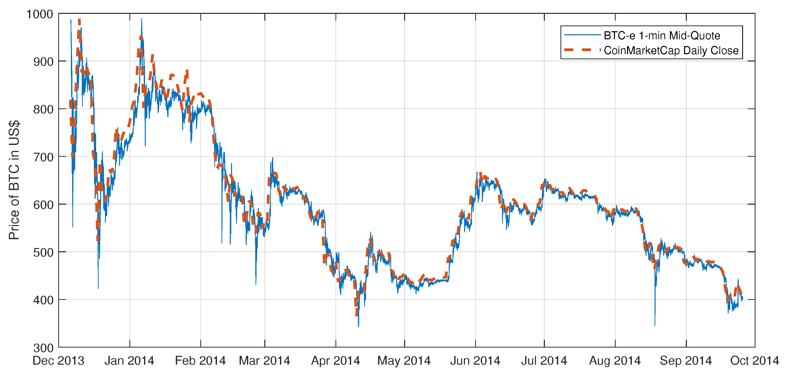
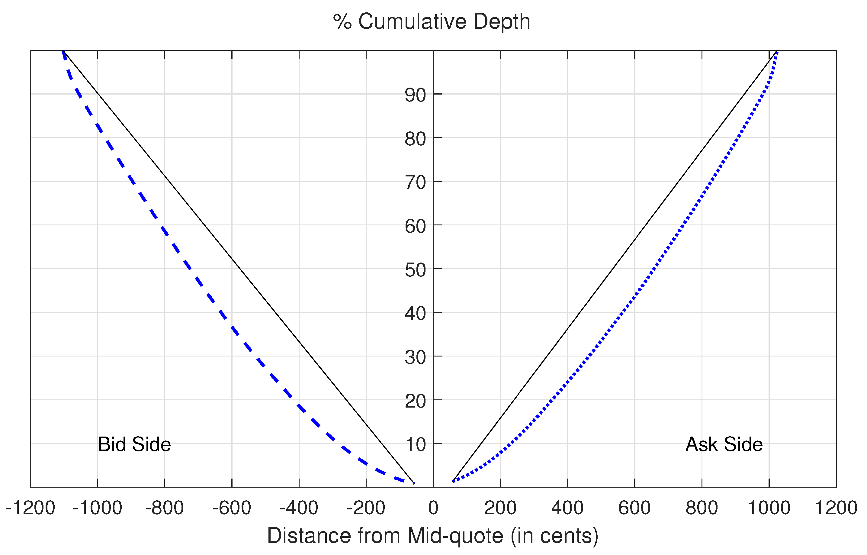
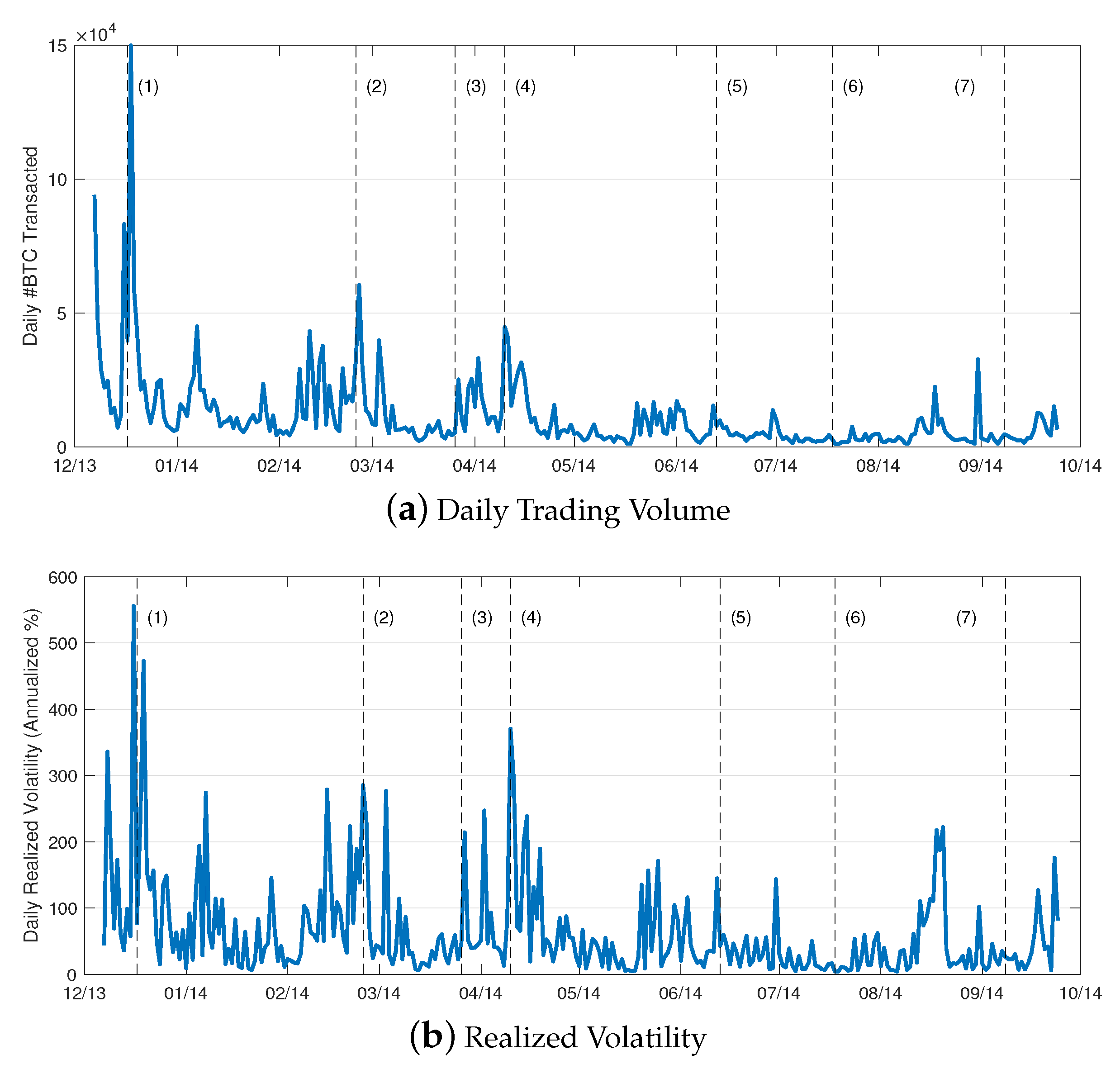
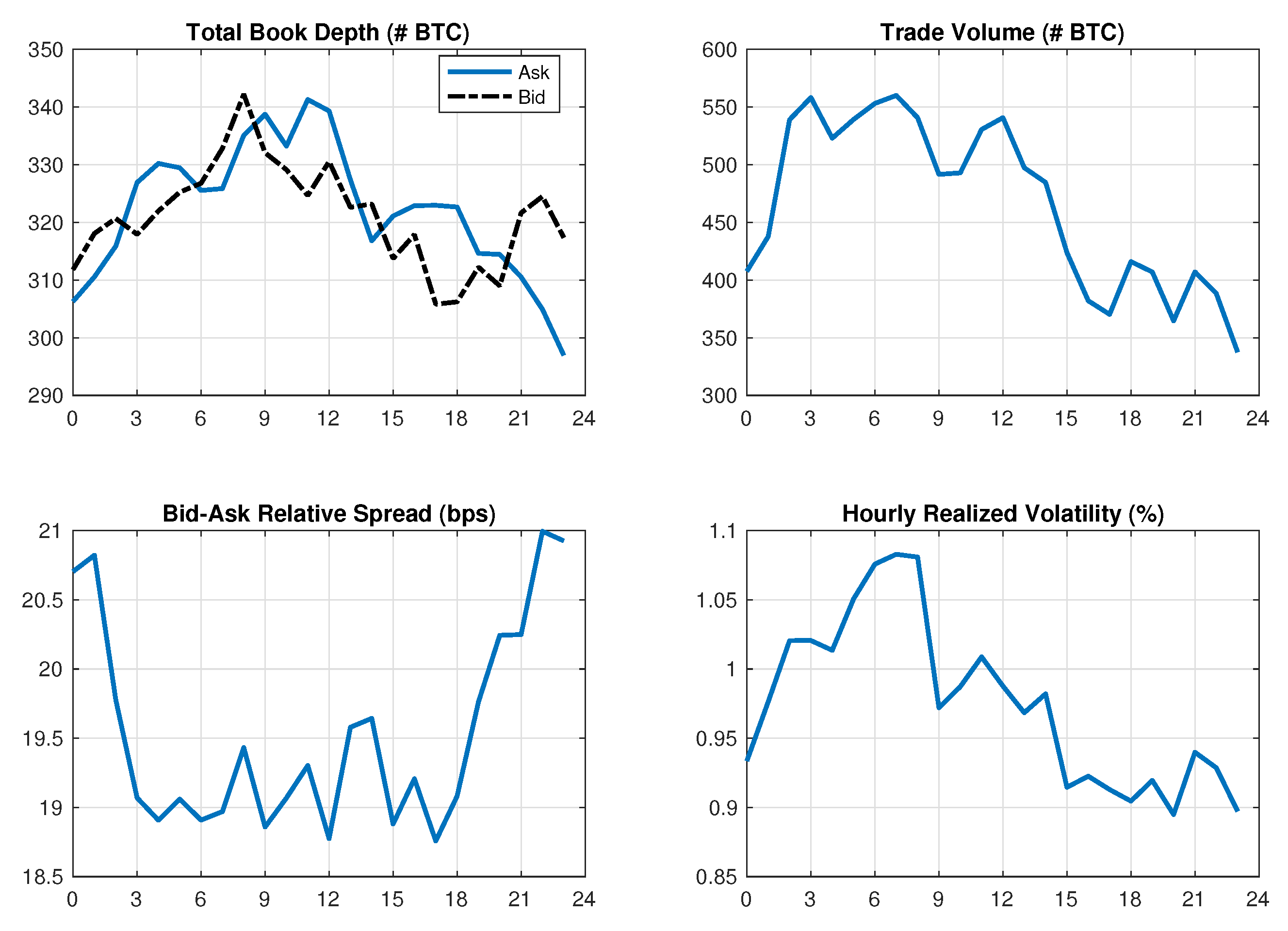
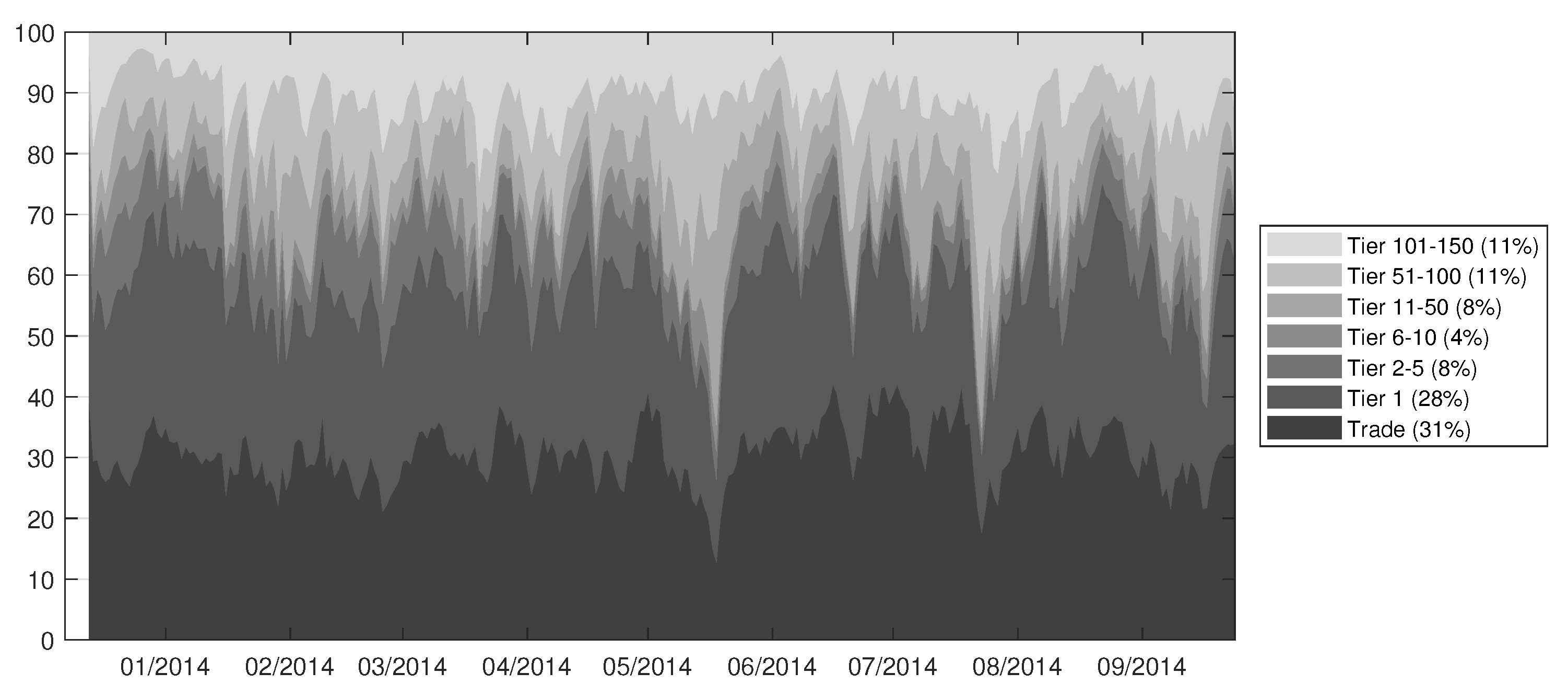
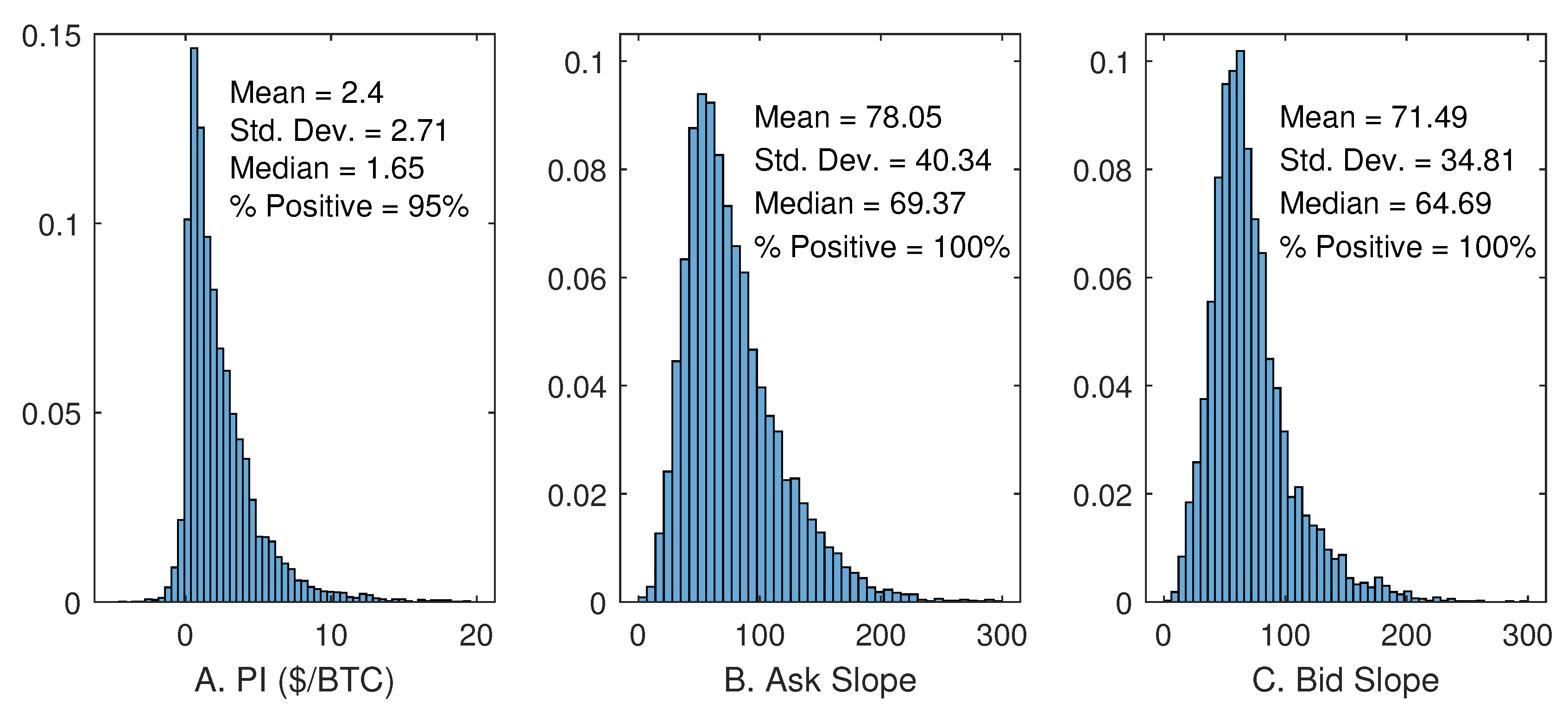
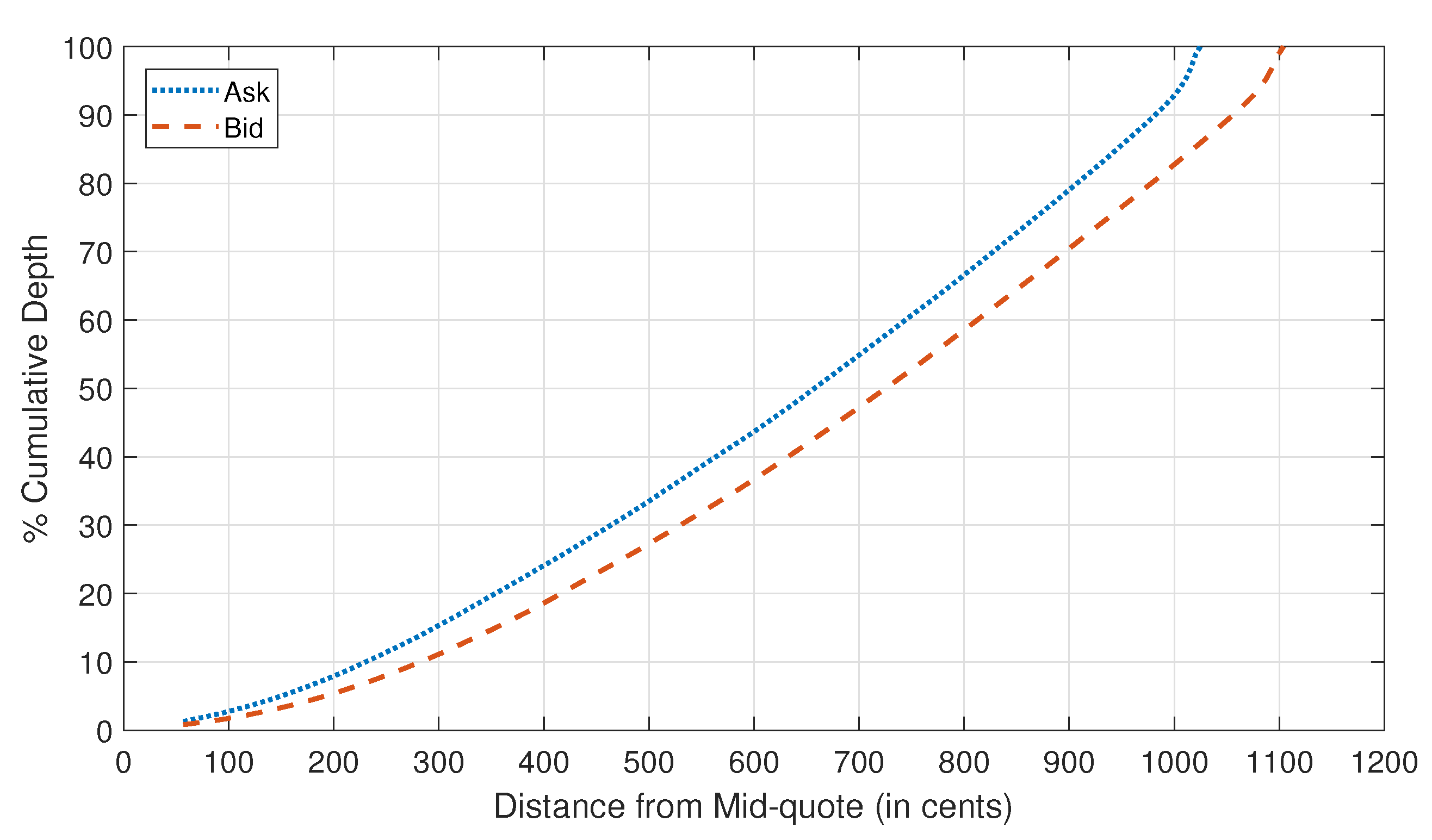
Table 1.
Summary statistics of BTC-e limit order book: 7 December 2013 to 24 September 2014.
| Variable | Tier 1 | Tier 5 | Tier 10 | Tier 20 | Tier 50 | Tier 100 | Tier 150 |
|---|---|---|---|---|---|---|---|
| Panel A: Distribution of Depth Across Price Tiers | |||||||
| Ask: Cum. Depth | 4.1 | 17.5 | 30.0 | 51.3 | 108.3 | 203.5 | 322.3 |
| Ask: % Cum. Depth | 1.3 | 5.4 | 9.2 | 15.6 | 33.0 | 61.9 | 100.0 |
| Bid: Cum. Depth | 2.6 | 11.1 | 19.8 | 36.3 | 89.3 | 190.6 | 321.3 |
| Bid: % Cum. Depth | 0.8 | 3.5 | 6.2 | 11.3 | 27.2 | 58.1 | 100.0 |
| Panel B: Spreads as Fraction of Bid-Ask Midpoint (bps) | |||||||
| Ask: Distance from Best Bid | 19.5 | 36.7 | 47.3 | 61.8 | 94.2 | 139.2 | 181.4 |
| Ask: Volume-weighted Spread | 19.5 | 27.6 | 33.9 | 42.8 | 62.2 | 88.6 | 116.6 |
| Bid: Distance from Best Ask | 19.5 | 36.1 | 46.5 | 61.1 | 95.0 | 144.9 | 194.3 |
| Bid: Volume-weighted Spread | 19.5 | 27.7 | 33.9 | 43.2 | 64.2 | 94.4 | 126.2 |
Table 2.
Descriptive statistics of daily trading activity. The reported statistics are based on BTC-e transaction history data over the period from 7 December 2013 to 24 September 2014. Each day is defined to be from 0:00:00 to 23:59:59 ET.
Table 2.
Descriptive statistics of daily trading activity. The reported statistics are based on BTC-e transaction history data over the period from 7 December 2013 to 24 September 2014. Each day is defined to be from 0:00:00 to 23:59:59 ET.
| Variable | Buyer-Initiated Trades | Seller-Initiated Trades | ||||||
|---|---|---|---|---|---|---|---|---|
| Mean | P5th | Median | P95th | Mean | P5th | Median | P95th | |
| Trade Frequency | 6710 | 1712 | 4413 | 15,220 | 6197 | 1179 | 3648 | 15,427 |
| Volume (# BTC) | 5626 | 873 | 3321 | 18,584 | 5752 | 795 | 3065 | 18,808 |
| Dollar Volume ($ m) | 3.44 | 0.49 | 1.939 | 11.21 | 3.51 | 0.44 | 1.76 | 11.27 |
| Trade Size (# BTC) | 0.84 | 0.01 | 0.10 | 3.25 | 0.93 | 0.01 | 0.10 | 3.78 |
| Dollar Trade Size ($) | 512.62 | 5.13 | 56.11 | 2007.58 | 566.87 | 5.50 | 59.93 | 2291.98 |
Table 3.
This table reports the information shares of trade and limit order prices. The price vector consists of last trade price, and depth-weighted prices of limit orders at tier 1, tiers 2–5, tiers 6–10, tiers 11–50, tiers 51–100, and tiers 101–150 on both sides of the market. Their dynamics at the one-minute frequency are modeled with a vector error correction model with 10 lags, and information shares are computed from the Cholesky decomposition of the covariance matrix of the residuals. The model is estimated separately for each day. Each day is defined to be from 0:00:00 to 23:59:59 ET. Data are from BTC-e for the period from December 7, 2013 to September 24, 2014. Panels A1, A2, and A3 report the means and standard errors of information shares separately for the high volatility, average volatility, and low volatility sub-samples partitioned as described in the text. Panel B1 reports the test statistics of the difference in mean information share of each order category on high-volatility days versus average-volatility days. Panel B2 reports the test statistics of the difference in mean information share of each order category on low-volatility days versus average-volatility days.
| Statistic | Trade | Tier | Tiers | Tiers | Tiers | Tiers | Tiers |
|---|---|---|---|---|---|---|---|
| 1 | 2–5 | 6–10 | 11–50 | 51–100 | 101–150 | ||
| A1. High volatility days (N=62) | |||||||
| Mean | 30.05 | 31.76 | 13.44 | 5.24 | 5.55 | 7.60 | 6.37 |
| S.e. | 1.11 | 1.03 | 0.70 | 0.39 | 0.51 | 0.90 | 0.88 |
| A2. Average volatility days (N=172) | |||||||
| Mean | 31.98 | 27.38 | 6.88 | 2.79 | 7.62 | 11.33 | 12.02 |
| S.e. | 0.90 | 0.79 | 0.37 | 0.22 | 0.63 | 0.92 | 0.94 |
| A3. Low volatility days (N=58) | |||||||
| Mean | 27.94 | 23.60 | 5.88 | 3.97 | 13.45 | 12.62 | 12.53 |
| S.e. | 1.72 | 1.50 | 0.71 | 0.54 | 1.76 | 1.88 | 1.45 |
| B1. Test of hypothesis 1A | |||||||
| t-stat | −1.357 | 3.366 | 8.303 | 5.496 | −2.552 | −2.910 | −4.381 |
| p-val | 0.088 | 0.000 | 0.000 | 0.000 | 0.006 | 0.002 | 0.000 |
| B2. Test of hypothesis 1B | |||||||
| t-stat | −2.085 | −2.225 | −1.242 | 2.025 | 3.129 | 0.619 | 0.293 |
| p-val | 0.020 | 0.014 | 0.109 | 0.023 | 0.001 | 0.269 | 0.385 |
Table 4.
Regression of limit order book slope on adverse selection and information environment indicators. The slope of the order book on each side is estimated from order book snapshot prevailing at the end of each hour. Adverse selection (‘PI’) is measured by the price impact of order book events over each hour, as described in the text. Days with large value shock (‘hivol’) have both realized volatility and high-low range measures in the top quartile of their respective distributions. Days with low value shock (‘lovol’) are similarly defined using the bottom quartile. Controls include the percent of same-side depth at the top tier, slope on the opposite side, the total quantity of all ask limit orders, the total quantity of all bid limit orders, total trading volume and log trade count over each hour split into buyer-initiated and seller-initiated, and hourly realized volatility computed from five-minute returns. All depth and trading volume variables are in the number of coins and log-transformed. Hourly dummies capture the time-of-day effects. Data are from BTC-e for the period from 7 December 2013 to 24 September 2014. , , .
| Dep. Variable = Ask Slope | Dep. Variable = Bid Slope | |||||||
|---|---|---|---|---|---|---|---|---|
| (1) | (2) | (3) | (4) | (5) | (6) | (7) | (8) | |
| PI | ** | ** | *** | *** | *** | *** | *** | *** |
| PI × hivol | ** | ** | ** | ** | *** | *** | *** | *** |
| PI I × lovol | *** | *** | *** | *** | *** | *** | *** | *** |
| Control Variables: | ||||||||
| Realized Volatility | *** | *** | *** | *** | *** | *** | *** | *** |
| Opposite Slope | *** | *** | *** | *** | *** | *** | *** | *** |
| % Depth at Top Tier | *** | *** | *** | *** | ||||
| Total Ask Depth (logged) | * | 1.05 | 0.90 | 0.82 | *** | *** | *** | *** |
| Total Bid Depth (logged) | *** | *** | *** | *** | *** | *** | *** | *** |
| Buyer-initiated Trade Volume (logged) | *** | *** | *** | *** | *** | *** | *** | *** |
| Buyer-initiated Trade Count (logged) | 1.03 | 1.19 | 1.13 | *** | *** | *** | ||
| Seller-initiated Trade Volume (logged) | *** | *** | *** | *** | *** | *** | *** | *** |
| Seller-initiated Trade Count (logged) | ** | ** | ** | 0.52 | 0.63 | 0.65 | ||
| Constant | Yes | Yes | Yes | Yes | Yes | Yes | Yes | Yes |
| Hourly Dummies | No | No | No | Yes | No | No | No | Yes |
| Nobs | 7007 | 7007 | 7007 | 7007 | 7007 | 7007 | 7007 | 7007 |
| Adjusted | 0.39 | 0.39 | 0.40 | 0.38 | 0.41 | 0.41 | 0.42 | 0.40 |
Table 5.
Regression of price impact on limit order book state. Panel A reports the baseline regression of price impact on listed explanatory variables capturing the prevailing state of the limit order book. We estimate the regression without (Model 1) and with (Model 2) hourly dummies to account for possible diurnality of price impact. , , . Panel B shows the incremental explanatory power of the 24-h history of each explatory power. Each row in Panel B is based on the regression that augments baseline model 1 with 24 lags of the given explanatory variable. Reported are the number of lags with significant coefficient at the 1%, 5%, and 10% level, as well as the adjusted . Price impact (the dependent variable in all regressions reported in the table) is the price impact of order book events over each hour, estimated as described in the text. Data are from BTC-e for the period from 7 December 2013 to 24 September 2014.
| Panel A: Baseline Regression of Price Impact | ||||
|---|---|---|---|---|
| Explanatory Variable | Model 1 | Model 2 | ||
| Ask Slope | −0.000 | −0.000 | ||
| Bid Slope | 0.001 | 0.000 | ||
| Total Ask Depth (logged) | *** | *** | ||
| Total Bid Depth (logged) | * | * | ||
| Buy Volume (logged) | *** | *** | ||
| Sell Volume (logged) | ** | ** | ||
| Realized Volatility | *** | *** | ||
| % Ask Depth at Top Tier | −0.007 | −0.007 | ||
| % Bid Depth at Top Tier | −0.010 | −0.010 | ||
| % Ask Depth at Top 5 Tiers | *** | ** | ||
| % Bid Depth at Top 5 Tiers | ** | ** | ||
| Hourly Dummies | No | Yes | ||
| Adjusted | 12.61 | 11.49 | ||
| Panel B: Explanatory Power of 24-h History | ||||
| Explanatory Variable | # Significant Lag Coefficients | |||
| 1% Level | 5% Level | 10% Level | Adj. | |
| Ask Slope | 0 | 0 | 0 | 10.04 |
| Bid Slope | 0 | 0 | 1 | 10.08 |
| Total Ask Depth (logged) | 0 | 0 | 0 | 9.95 |
| Total Bid Depth (logged) | 1 | 1 | 3 | 10.27 |
| Buy Volume (logged) | 0 | 1 | 4 | 10.24 |
| Sell Volume (logged) | 0 | 1 | 1 | 10.27 |
| Realized Volatility | 1 | 2 | 3 | 9.69 |
| % Ask Depth at Top Tier | 0 | 2 | 3 | 10.15 |
| % Bid Depth at Top Tier | 0 | 1 | 2 | 10.08 |
| % Ask Depth at Top 5 Tiers | 0 | 0 | 1 | 10.07 |
| % Bid Depth at Top 5 Tiers | 0 | 0 | 0 | 9.98 |
© 2019 by the authors. Licensee MDPI, Basel, Switzerland. This article is an open access article distributed under the terms and conditions of the Creative Commons Attribution (CC BY) license (http://creativecommons.org/licenses/by/4.0/).
Share and Cite
MDPI and ACS Style
Ghysels, E.; Nguyen, G. Price Discovery of a Speculative Asset: Evidence from a Bitcoin Exchange. J. Risk Financial Manag. 2019, 12, 164. https://doi.org/10.3390/jrfm12040164
AMA Style
Ghysels E, Nguyen G. Price Discovery of a Speculative Asset: Evidence from a Bitcoin Exchange. Journal of Risk and Financial Management. 2019; 12(4):164. https://doi.org/10.3390/jrfm12040164
Chicago/Turabian StyleGhysels, Eric, and Giang Nguyen. 2019. "Price Discovery of a Speculative Asset: Evidence from a Bitcoin Exchange" Journal of Risk and Financial Management 12, no. 4: 164. https://doi.org/10.3390/jrfm12040164