Modeling the Impact of Agricultural Shocks on Oil Price in the US: A New Approach


1
Business and Economics Research Group, Ho Chi Minh City Open University, Ho Chi Minh City 7000, Vietnam
2
School of Advanced Study, Ho Chi Minh City Open University, Ho Chi Minh City 7000, Vietnam
*
Author to whom correspondence should be addressed.
J. Risk Financial Manag. 2019, 12(3), 147; https://doi.org/10.3390/jrfm12030147
Submission received: 29 June 2019
/
Revised: 28 July 2019
/
Accepted: 2 August 2019
/
Published: 10 September 2019
(This article belongs to the Special Issue Energy Finance and Sustainable Development)
Abstract
:The current literature has generally considered prices of the agricultural commodity as an endogenous factor to crude oil price. As such, the role of the agricultural market in the energy sector has been largely ignored. We argue that the expansion of agricultural production may trigger a significant increase in oil price. In addition, the world has recently witnessed a growth in biofuel production, leading to an increase in the size of the agricultural sector. This study is conducted to examine the impact of different agricultural shocks on the oil and agricultural markets in the US for the period from 1986 to 2018. The study utilizes the Structural Vector Autoregressive (SVAR) model to estimate the relationship between the agricultural market and the crude oil market. Moreover, the variance decomposition is also used to quantify the contribution of agricultural demand shocks on oil price variations. Findings from this paper indicate that different agricultural shocks can have different effects on oil price and that corn use in ethanol plays an important role in the impact of corn demand shocks on oil price. We find evidence that the agricultural market can have an impact on oil prices through two main channels: indirect cost push effect and direct biofuel effect. Of these, the biofuel channel unexpectedly suggests that the expansion of bioethanol may in fact foster the dependency of the economy on fossil fuel use and prices.
1. Introduction
The correlation of crude oil price and agricultural commodity prices during the food price crisis of 2007–2008 has led to a rich array of studies on the impact of crude oil price and biofuel expansion on agricultural prices. According to these studies, the increase in crude oil price has increased the prices of many agricultural crops and damaged global food security, as crude oil is one of the main factors of agricultural production (Bayramoğlu et al. 2016; Persson 2015; Adam et al. 2018; Wang et al. 2014). Furthermore, the increase in crude oil price also raised the demand for biofuel as an alternative energy source. The coincidence of biofuel expansion and the occurrence of the food price crisis during 2007–2008 has raised serious concerns about the causality from the former to the latter (Lucotte 2016; Ma et al. 2016; Ahmadi et al. 2016). In particular, the increase in biofuel production has led to an increase in corn demand, as corn is the main feedstock of bio-ethanol in the US. The increase in corn demand led to an increase in corn price and the prices of other agricultural commodities, as these crops compete for planted acreage and other agricultural resources (Wang et al. 2014). Furthermore, the demand for biofuel was strengthened as many developed countries imposed several renewable energy mandates, which greatly increased biofuel consumption. Since then, biofuel has played a key role in connecting the agricultural market and the energy market (De Gorter et al. 2013).
However, the correlation between crude oil price and agricultural commodity prices does not always mean causation from the former to the latter. Previous studies often focused on the causality from crude oil price to agricultural commodity prices, so the possibility of reverse causality is often ignored in the literature. Baumeister and Kilian (2014) argued that the mechanization of agricultural production may increase the energy consumption in the agricultural sector. Therefore, an increase in agricultural production is likely to increase fuel demand and crude oil price. Moreover, an increase in the size of the agricultural and biofuel sectors makes the reverse causality more likely to happen.
Despite its scarcity, the empirical literature has recognized the causality from food prices to energy prices (Su et al. 2019; Vacha et al. 2013; Avalos 2014; Natanelov et al. 2011; Zhang et al. 2010). However, these studies often employed only the price data without including further information about the agricultural supply and demand. Baumeister and Kilian (2014) and Serra and Zilberman (2013) criticized these time-series models for their inability to identify the transmission mechanisms of the price spillovers between the two markets. Theoretically, the agricultural sector can influence crude oil price through both indirect input cost and direct biofuel channels (Ciaian 2011). The author showed that the two channels can have different impacts on the crude oil price. In particular, the increase in agricultural supply may lead to a decrease in crude oil demand and crude oil price. However, the increase in agricultural demand caused by ethanol expansion may either increase energy demand or increase energy supply. Therefore, we find that the existing empirical studies are inconclusive about the transmission mechanisms in which the agricultural market can influence the crude oil price.
The contribution of this paper is twofold. Firstly, we confirm the results derived from the theoretical model in Ciaian (2011) that different shocks from the agricultural market can have different effects on oil price. We use the agricultural supply and demand shocks of different crops to test the existence of the indirect input cost and the direct biofuel channels. Our results confirm the existence of the indirect input cost channel in the barley market and the direct biofuel channel in the corn and sorghum market. For the corn market, we identify that agricultural demand shocks play a larger role in the fluctuation of crude oil price, compared to the effect of the agricultural supply shock.
Secondly, our results have important policy implications for the biofuel sector. We find that an increase in corn use in ethanol can have a positive influence on the crude oil price. This is in contrast to the original expectation that the expansion of biofuel can increase the total fuel supply and reduce the dependency of the domestic economy on fossil fuel. Our results show that an increase in corn use in ethanol may lead to an increase in fuel demand and crude oil price, which is an unexpected consequence of biofuel. Such conclusions could not be reached if the analysis only included agricultural prices.
Moreover, the use of corn in ethanol has an additional advantage over using corn price in the sense that corn price and crude oil price are likely to react to changes in monetary and trade policies, global business cycle, and aggregate demand. However, the expansion of corn use in ethanol is most likely to be the result of the renewable energy mandate, which is exogenous to changes of the macroeconomic variables. Therefore, the impact of corn use in ethanol on crude oil price is not likely to be correlated with global economic events.
In general, the novelty of our study is that we include variables which are different in nature, such as oil prices, agricultural prices, agricultural supplies, and corn use in ethanol. This approach differs from existing studies, that often focus on the price spillover effects between the two markets. Our approach is interesting because we can observe a number of interconnected relationships, which might be missed if the analysis only included price variables. In particular, we confirm that the agricultural market can have feedback effects on oil prices. Previous studies did not disentangle the impact of agricultural supply and demand shocks, which can potentially have different effects on oil prices, according to Ciaian (2011). By observing variables other than prices, we find evidence that the agricultural market is more likely to affect oil prices through the direct biofuel channel. We also find that biofuel expansion can lead to an increase in agricultural production, which will eventually increase oil demand.
The following section of this paper is a review of the studies related to the current research. Section 3 presents the methodology and the models used in the empirical section. Section 4 shows the data and preliminary tests. Section 5 presents the results of the empirical analysis and the discussion of the outcomes. Section 6 concludes our research.
2. Literature Review
The literature on the nexus of food versus energy often investigates the relationship between biofuel, agricultural commodity, and crude oil prices. Regarding the studies on biofuel and agricultural markets, many efforts have been devoted to research on price and volatility transmission. Many studies have shown that shocks from the corn market can have an impact on ethanol price, due to corn being a feedstock of bioethanol. Kristoufek et al. (2016) employed the wavelet coherence methodology to study the relationship between ethanol and agricultural commodities in the US and Brazil. The results show that the impact of corn price on ethanol price is unidirectional. The relationships are robust, both in short- and long-term periods. Similarly, Dutta et al. (2018) argued that the volatility in the corn market can have an impact on ethanol price. The paper employed conditional Generalized Autoregressive Conditional Heteroskedasticity (GARCH)-jump models with daily US ethanol and corn prices, both series are based on future contracts. The study found that the relationship is asymmetric because only positive shocks on corn price volatility can induce an increase in ethanol price. Bentivoglio et al. (2016) employed a vector error correction model with the Granger causality test, impulse response function, and forecast error variance decompositions to illustrate that ethanol price is impacted by fluctuations in oil and corn prices, but not the reverse. Dutta (2018) also showed similar results using the Autoregressive Distributed Lag (ARDL) model and the Kyrtsou–Labys nonlinear causality test.
On the other hand, Hao et al. (2017) showed that the ethanol market can also impact agricultural commodity prices. The authors focused on the consequences of biofuel production expansion in the US on the welfare of the poor in developing countries. Hao et al. (2017) investigated the influences of the US ethanol market on the maize prices of developing countries using the panel structural vector autoregression model (panel SVAR). The study divided the developing countries into groups with different political and geographical characteristics, which have potential impacts on the vulnerability of these countries to changes in the US ethanol and maize market. The authors found that the dependency of a country on US Food Aid may have a positive impact on the response of domestic maize prices to US ethanol supply shock. Similarly, coastal countries were found to be more likely to be affected by US ethanol demand shock.
Some studies pointed out that the causal relationship between the agricultural and ethanol markets can run in both ways. Apergis et al. (2017) employed a threshold error correction model (TECM) to show that biofuel and agricultural commodity prices have a bi-directional causal relationship. The study used the daily prices of seasonal biodiesel and agricultural commodities, including corn, sugar, sugarcane, soybean oil, sunflower oil, palm oil, and camelina oil. The results show that the relationships between biofuel price and agricultural commodity prices are non-linear. The non-linear relationships suggest that the analysis of the relationship should be divided into two periods, where the two markets have a stronger bond during the second periods. Chiu et al. (2016) confirmed a bidirectional relationship between corn and ethanol price using the Granger causality test and impulse response function in the Vector Autoregressive (VAR) model and Vector Error Correction Model (VECM).
Most of the studies on this relationship focused on price transmissions. However, there are studies confirming the volatility spillover effect. Chang et al. (2018) showed that there is a strong volatility transmission between the bioethanol market and the agricultural markets. The study employed the diagonal BEKK (named after the authors of the model: Baba, Engle, Kraft, and Kroner) to investigate the spot prices and future prices of corn, sugarcane, and bioethanol. The results show that future prices of bioethanol and agricultural commodities have stronger co-volatility spillovers than their spot prices. These outcomes suggest that the future prices can be used for risk management purpose. Saghaian et al. (2018) also confirmed the volatility spillover between the corn and ethanol markets. The authors showed that the relationship is bidirectional. However, the spillover effect from the ethanol to the corn market can only be observed using the daily data.
Enciso et al. (2016) employed the Aglink-Cosimo model to investigate the impact of removing biofuel-related policies on the biofuel and agricultural commodity prices and volatilities. According to their results, the biofuel policies can increase biofuel production, consumption, and prices, and reduce their volatilities. Similarly, Zhou and Babcock (2017) showed that corn prices could decrease 5% or 6% if the US biofuel mandates were to be reduced, using the competitive storage model.
The food versus fuel nexus also attracts many studies on the relationship between agricultural commodity and crude oil prices. In this literature, VAR models have been widely used to capture the impact of crude oil price changes on agricultural commodity prices (Lucotte 2016; Ma et al. 2016; Ahmadi et al. 2016). Some studies included the exchange rate and the global business cycle in the analysis of the relationship, as these variables can have an effect on both crude oil and agricultural commodity price (Adam et al. 2018; Wang et al. 2014; Vo et al. 2019). Adam et al. (2018) employed a vector autoregressive model (VAR) to analyze the crude oil price, the rice price, and the exchange rate. Their results show that crude oil price has a unidirectional relationship with rice price, however, the relationship only exists in the short term. The reason is that oil price changes can cause fluctuations in rice price, because crude oil is an important input factor in rice production.
The relationship between crude oil and agricultural commodity prices was impacted by the food price crisis during 2007–2008. Wang et al. (2014) used the SVAR approach to analyze the impact of different oil-related shocks on various agricultural commodity prices. SVAR approach has been widely used as well (Vo et al. 2018; Nguyen and Vo 2019). The study found that the impact of oil-specific demand shocks on the many agricultural commodity prices was only significant after the food price crisis. Han et al. (2015) also argued that the changes in crude oil price and agricultural commodity price relationship are most likely to be affected by the last financial crisis, of 2007–2008. Their analysis employed the multivariate normal mixture models to analyze the interactions of energy price and agricultural commodity prices. Their results show that industrial commodity prices are more likely to affect one another when the price and volatility transmission have a higher possibility to happen after the financial crisis. Using a VECM model, Chen and Saghaian (2015) showed that the relationship between oil, ethanol, and sugar has become stronger after 2008 in Brazil, where oil price tends to impact the other two variables, while sugar price tends to impact ethanol price. Most of the studies capturing the correlation between oil and agricultural markets interpret such correlations as the transmissions and spillovers from the former to the latter (Koirala et al. 2015; Zafeiriou et al. 2018; Allen et al. 2018).
The reason for the stronger bond between the two markets might be caused by renewable energy mandates. Several studies argued that the expansion of biofuel production has attracted land use, water, and other agricultural resources. Because these resources are limited, the expansion may lead to the reduction of food crop supplies (Büyüktahtakın and Cobuloglu 2015; De Martino Jannuzzi 1991; Fradj and Jayet 2016; Herrmann et al. 2017). To and Grafton (2015) provided evidence that a global increase in oil price and biofuel demand has contributed a significant role in agricultural commodity price fluctuations.
On the other hand, some studies also recognized the potential impact of agricultural shocks on the crude oil price. Ciaian’s theoretical model (Ciaian 2011) suggests that agricultural shocks can affect crude oil price through different channels. According to this study, when food demand is inelastic, surges in agricultural supply resulting from positive productivity shocks accompanied may reduce the farmers’ profit margin and therefore trigger a reduction in production activities and fuel demand. On the contrary, with an elastic food demand, an increase in agricultural productivity may result in an increase in fuel demand, due to the increase in food consumption. Besides the indirect input cost channel, the theoretical framework shows that an increase in biofuel production can lead to opposite effects on crude oil price. On the one hand, biofuel expansion will increase the energy supply and have a negative effect on crude oil price. On the other hand, agricultural production expansion due to an increase in demand for ethanol feedstock will increase fuel demand and crude oil price. In general, the direct biofuel channel has an ambiguous effect on crude oil price.
Su et al. (2019) showed that the bidirectional relationships between crude oil price and agricultural commodity prices are more likely to be found in the sub-sample periods using the sub-sample rolling estimation. Furthermore, the study also pointed out that agricultural commodities that are not feedstocks of biofuel production can also have bidirectional relationships with oil price.
The existing studies suggest the increasing roles of agricultural shocks in energy markets, specifically the ethanol and crude oil markets. It has been shown that agricultural shocks can be divided into supply and demand shocks, with each type of shock having potentially different impacts. However, the existing studies only employed agricultural commodity prices to investigate the relationship between agricultural and energy markets. Within the extent of our knowledge, our study is the first one to attempt to investigate the impact of agricultural shocks on oil price using agricultural demand and supply shocks. The study reveals that supply and demand shocks can have different impacts on oil price and thus, should be studied individually.
3. Methodology
In this paper, we used the SVAR model to estimate the relationship between agricultural markets and the crude oil market. It has been pointed out that agricultural commodity prices are endogenous to oil price, and vice versa (Zhang et al. 2010; Natanelov et al. 2011; Vacha et al. 2013; Avalos 2014; Su et al. 2019). Therefore, standard regression models cannot capture the bidirectional relationship between the two commodities. Even though VAR models can be used to treat the endogeneity problem, such models are said to have little power to establish a causal relationship between oil and agricultural commodity prices (Baumeister and Kilian 2014). Cooley and LeRoy (1985) pointed out that the estimations of VAR models are often based on ad-hoc assumptions, which may be arbitrary. Thus, we employed the following SVAR model, with exclusion restrictions based on the economic theories and empirical evidence:
In the first model, we have , where denotes the logs of world crude oil production, denotes the aggregate demand captured by the Kilian’s index (Kilian 2018), denotes the US real imported crude oil price, and represents the real agricultural commodity prices. represents the vector of mutually uncorrelated structural shocks in each equation of the system. is the first order difference operator. We ran this model on the full sample period from January 1986 to May 2018.
We imposed matrix so that its inverse had the following recursive structure:
The reduced-form of Equation (1) becomes:
where .
We ran the SVAR model for the vector for the second model, where denotes the agricultural supplies of corn, sorghum, and barley. We ran the third model for the vector ), where denotes the logs of corn use in ethanol, denotes the corn price, and represents the corn supply.
The orders of the variables in the vectors reflect the exclusion restrictions, which are widely agreed in the economic theories and empirical literature. Firstly, studies on the link between the oil market and the agricultural markets often agreed on the exogeneity of the former to the latter (Kilian 2009; Wang et al. 2014; Qiu et al. 2012; McPhail et al. 2012; Mcphail 2011; To et al. 2019). Therefore, oil-related variables have higher orders in the vector of endogenous variables. Within the oil market, oil supply is assumed to only respond to its own shock within the same period. This assumption is based on the fact that major oil producers often have a long-term plan for their production. Therefore, these oil producing countries do not respond to temporary fluctuations in demand shock. The global economic activities often respond to the disruptions of oil supply caused by political events from the Organization of Petroleum Exporting Countries (OPEC), while the global oil supply does not respond contemporarily to the aggregate demand shock. On the other hand, oil prices do not have a contemporaneous impact on the global industrial demand, while the aggregate demand can have an impact on oil demand, as reflected by Kilian (2009).
Within the agricultural market, agricultural demand shocks often have a stronger impact on agricultural commodity prices than agricultural supply shocks (Qiu et al. 2012). The reason is that the agricultural stocks and trade liberalization tend to lessen the impact of agricultural supply shocks on crop prices (Jha and Srinivasan 2001). Therefore, the agricultural prices and corn use in ethanol have a higher order of exogeneity than the agricultural supply variables. For the third model, the response of ethanol demand to shocks to the corn market is considered lagging because ethanol demand is more likely to be affected by the renewable energy mandates (Qiu et al. 2012; McPhail et al. 2012), which explains the exogeneity of corn use in ethanol to other corn demand shocks.
The fluctuations of the global aggregate demand, crude oil demand, and supply shocks, which are often the results of an increase in trade openness, changes in monetary and trade policies, contribute simultaneously and significantly to the fluctuation in demand for agricultural products and crude oil price. The SVAR helps us to disentangle the impact of the agricultural supply and demand shocks from the common factors by decomposing the error terms into mutually uncorrelated shocks.
4. Data and Tests
The main purpose of this paper is to investigate the impact of different agricultural shocks on the US crude oil price over the period from January 1986 to May 2018. In this paper, we used the imported crude oil price to capture the domestic oil price. The real monthly average imported crude oil price and world crude oil production were obtained from the Energy Information Administration (EIA) (https://www.eia.gov/). The nominal agricultural commodity prices, agricultural supplies, and corn use in ethanol were collected from the Feed Grains Database of Economic Research Service, USDA (https://www.ers.usda.gov/). The nominal agricultural commodity prices were deflated by the Consumer Price Index of the total all items for the United States, retrieved from the Federal Reserve Economic Data (FRED) (https://fred.stlouisfed.org). By using the real prices of agricultural commodities and crude oil, we effectively controlled for the simultaneous inflationary effects of monetary policies on both commodity prices. Therefore, we can disentangle the effects of the agricultural supply and demand shocks from the common factor of monetary policies. The changes in global demand for industrial commodities can be captured by the changes in demand for transport services, which are reflected in the variation in ocean freight rate (Kilian 2009). Therefore, we used an index developed by Kilian (Kilian 2018) as a proxy for the aggregate demand1.
Regarding the decision of structural breaks and subsample periods, we recognize that there are other important economic and political events that might have a significant impact on crude oil and agricultural prices. For example, Baumeister and Kilian (2016) stated in their work that several supply and demand shocks during 2014 played a large role in the fluctuations of the oil price and other commodities. During this year, the production expansion of both OPEC and non-OPEC countries increased the global oil supply. Additionally, the price reduction of other commodities and the decline in oil stocking behaviors put downward pressure on the oil demand. On the other hand, Chiu et al. (2016) recognized that the relationship between crude oil prices and agricultural prices has changed over time due to multiple structural shifts. In particular, the authors observed that the causal relationship from agricultural prices to oil prices was strengthened during 1998–1999 (after the Asian financial crisis) and 2008–2009 (during the Global financial crisis and Global food crisis). As a result, we recognize that these events are worthy of exploration for future research. However, we decided to focus on the impact of the Energy Policy Act of 2005 on the relationship between oil prices and the agricultural market in this paper.
For the first model, we divided the full sample into two subsamples, including the first period, from January 1986 to December 2005, and the second period, from January 2006 to May 2018. Barley, corn, and sorghum supply series were only available in quarterly data. For the second model, the marketing year of barley supply began on 1 June, and its four quarters included June–August, September–November, December–February, and March–May. Therefore, the first period of barley supply series was Q3 1985 to Q3 2005 and the second period was from Q4 2005 to the Q4 2017 in the barley marketing year. Similarly, the marketing year of corn and sorghum supply began on 1 September, and its four quarters included September–November, December–February, March–May, and June–August. Thus, the first period of corn and sorghum supply was from Q2 1985 to the Q2 2005 and their second period was from Q3 2005 to Q3 2017 in the corn and sorghum marketing year. For the third model, the first period of corn use in ethanol was from Q1 1986 to Q2 2005 and its second period was from Q3 2005 to Q3 2017 in the corn marketing year.
The partition of the dataset was motivated by the implementation of the Energy Policy Act of 2005. Previous studies pointed out that agricultural and energy markets are more likely to interact with each other after the event (Su et al. 2019; Avalos 2014; Wang et al. 2014; Baumeister and Kilian 2014). Moreover, the shocks of the food crisis and the global financial crisis, which can trigger changes in the joint dynamics between the two markets, also happened during this period. Baumeister and Kilian (2014) argued that the increase in the mechanization of the agricultural production in major agricultural countries can also increase the strength of the relationship between the agricultural and fuel markets. Therefore, the causal relationship from the former to the latter, if any, is more likely to be found during this period, compared to the previous periods.
Table 1 shows the descriptive statistics of the commodity prices, the agricultural supplies, and corn use in ethanol. The commodity prices had higher means and standard deviations during the second period. For each period, corn supply was larger in mean and more volatile than the supplies of other agricultural commodities. Moreover, the mean and volatility of the corn supply increased, while those of the barley and sorghum supplies decreased during the second period. Similarly, there was also an expansion of alcohol supply for fuel use during the second period.
In our structural VAR model, we decomposed the agricultural commodity price variance into agricultural supply shock and agricultural demand shocks in the second model. The third model further divided the corn demand shocks into corn use in ethanol shock and other corn demand shocks. For the oil market, we decomposed oil-related shocks into oil supply shock, aggregate demand shock, and other oil-specific demand shocks.
In this paper, we used the unit root tests based on the augmented Dickey and Fuller (ADF) (Dickey and Fuller 1979), Phillips and Perron (PP) (Phillips and Perron 1988), and Kwiatkowski–Phillips–Schmidt–Shin (KPSS) methods (Kwiatkowski et al. 1992). The null hypothesis of the ADF and PP tests is that the time series has a unit root, while the null hypothesis of the KPSS test is that the time series is stationary. For the ADF test in Table 2A, we cannot reject that 7 out of 10 series were non-stationary at 5% significance level. According to the PP test, there were 5 series that had a unit root. The KPSS statistics reject the hypothesis that nine series followed stationary processes. For the first order difference series, the three tests indicate stationarity at 1% significance level for all series, except for the KPSS statistics of the corn use in ethanol.
The conventional unit root tests may fail to reject the unit root hypothesis when the alternative stationarity is true and the series contains structural breaks. Taking account of this possibility, many studies have come up with unit root tests with structural breaks. These tests are more likely to reject the null hypothesis of unit root compared to the traditional Dickey–Fuller unit root test (Zivot and Andrews 2002; Perron 1989). However, the limitation of the model using one structural break is that it may still fail to reject the null hypothesis if the series contains two structural breaks (Perron and Vogelsang 1992; Clemente et al. 1998; Lumsdaine and Papell 1997). Moreover, according to Lee and Strazicich (2003), the null hypothesis of these models assumes a unit root without breaks. Therefore, rejection of the null hypothesis does not necessarily mean that the series is trend-stationary with breaks. In contrast, the rejection of the null suggests that the series may contain a unit root with breaks.
In Table 2B, we employed the unit root test with the assumption that the series contained a structural break developed by Zivot and Andrews (2002). The test has three models with different assumptions. The first model assumes that the time series has a structural break in the intercept, the second model assumes a structural break in trend, while the third model tests the stationarity of the series under the assumption of both intercept and trend. The three models show that most of the time series is integrated with the order of one.
5. Empirical Results
5.1. Agricultural Commodity Price and Oil Price Shocks
In the literature of crude oil price and its relationship with agricultural commodity prices, several studies found it helpful to add oil supply and global economic activity as control variables (Kilian 2009; Wang et al. 2014). The reason for this is that oil price might be endogenous to oil supply and the global business cycle, while the global business cycle can affect both oil and agricultural commodity prices. Following previous studies, we first investigated the price relationship using the monthly data and the following model, during the period from 1986m1 to 2018m5:
We considered the Akaike information criterion (AIC) to choose the optimal number of lags. The information criterion suggests two lags for the period 1986m1 to 2005m12 and one lag for the period 2006m1 to 2018m5. Figure 1A,B plots the accumulative response of agricultural commodity prices to the oil-specific demand shocks and the responses of oil price to agricultural commodity price shocks. During the first period, we can see that the agricultural commodity prices did not respond significantly to oil-specific demand shock. The only exception is the marginally significant response of corn price in the second month. However, the effect disappears shortly after that.
The situation changed sharply during the second period. The responses of corn price and sorghum price were positive and statistically significant, while the response of barley price was still insignificant. The response of corn price was significant in a very short period of time, while the effect on sorghum price lasted for 8 months.
Regarding the impact of agricultural shocks on oil price, there was no significant response during the first period. During the second period, the impact of barley-related shocks was still insignificant. On the other hand, corn-related shocks inflicted a significant and lasting impact on oil price (up to 8 months), while the effect of sorghum-related shocks was only marginally significant in the first month.
In general, the relationship between crude oil and agricultural commodity prices depends on the time period and the commodities under investigation. The links between the two markets appear to have been stronger during the second period. There are many studies attributing the difference between the two periods to the expansion of biofuel production. According to our results, corn and sorghum appear to have a stronger connection with crude oil price, compared to barley. In the US, corn and sorghum are used as feedstocks for biofuel production. Thus, these commodity prices are more likely to react to oil price fluctuations, as well as to trigger changes in the oil market.
The results suggest that the corn market can have an influence on crude oil price. According to the descriptive statistics, corn has far a larger supply than other agricultural commodities, which suggests that corn production may consume more energy than other agricultural sectors. In the US, corn is the main source of feedstock for ethanol production. Since 2006, the Energy Act 2005 by the US Government has increased ethanol consumption exponentially. The expansion of corn production due to an increase in ethanol consumption might explain why corn price can have an influence on oil price.
5.2. The Responses of Agricultural Commodity Prices to Supply and Demand Shocks
In the second model, our main objective was to differentiate the effects of agricultural shocks on oil price changes. According to the previous section, it has been shown that shocks in the agricultural markets can have a significant impact on crude oil price. However, agricultural shocks can be divided into supply and demand-related shocks. Therefore, using only agricultural commodity prices does not allow us to identify which agricultural shocks are responsible for crude oil responses. Thus, it is helpful to include agricultural supplies in the model specification, along with agricultural commodity prices. Similar practices can be found in Qiu et al. (Qiu et al. 2012). We used the following model:
In this model, we used the dummy variables as the exogenous variables of the SVAR system to control for the seasonality in agricultural supplies. The inclusion of the exogenous variables helped to increase the stability of the models, which tend to be unstable due to the inclusion of the agricultural supply data2. In Qui et al. (Qiu et al. 2012), the authors used the cubic spline interpolation to convert the quarterly agricultural supplies into monthly supplies. The disadvantage of this technique is that there should be a good theoretical reason for why the agricultural supply data should behave like a cubic function. In this paper, we decided to use the quarterly data of the agricultural supplies and the quarterly average of the other monthly variables. The consideration of the Akaike information criterion suggests four lags in both periods.
In prior to analyze the effects of agricultural shocks on oil price, we first plotted the response of agricultural commodity prices to the supply and demand shocks in Figure 2A–C. We can see that the responses of corn and sorghum price to real economic activity shocks are positive but not significant, while the impact of aggregate demand on barley price is marginally significant.
The shocks to barley, corn, and sorghum supplies did not have a significant impact on their own prices. In contrast, agricultural-specific demand shocks were the main factors contributing to the agricultural commodity price fluctuations. It can be seen that the responses of barley, sorghum, and corn price to their own specific demand shocks were positive and significant for eight quarters. The results confirm the hypothesis that the supply shock has a lesser impact on agricultural commodity prices than the demand shocks. The reason for this might be buffer stocking behaviors and trade liberalization. In times of crisis, the lack of supply from one region can be neutralized by the abundant supplies from other regions, thanks to free trade.
5.3. The Responses of Oil Price to Agricultural Supply and Demand Shocks
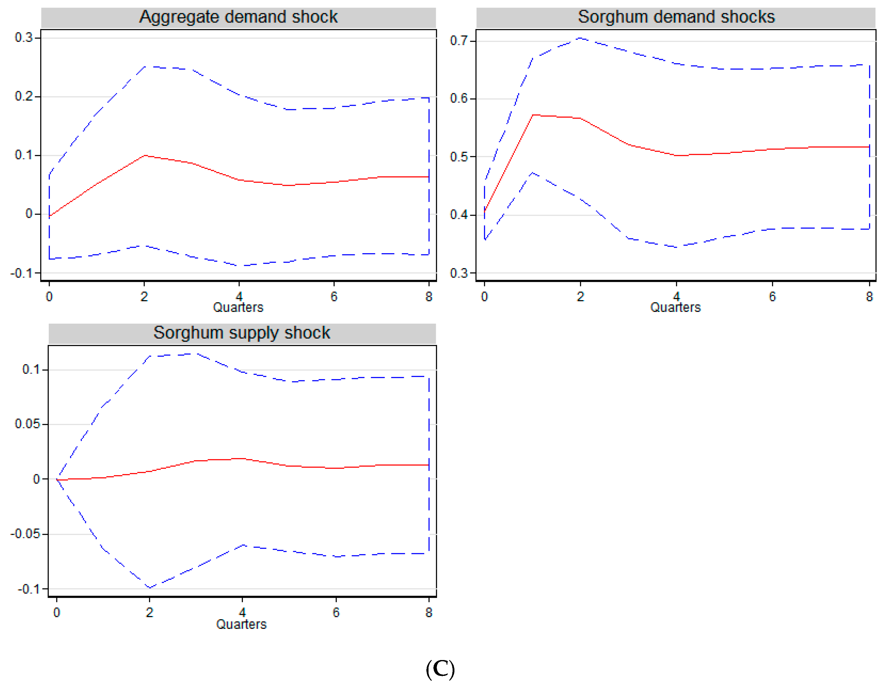
In the previous section, we analyzed the impacts of agricultural shocks on agricultural commodity prices. In this section, we will investigate the impact of these shocks on crude oil price. Figure 3A–C shows the responses of crude oil price to different agricultural shocks. During the first period, we can see that the oil price did not respond significantly to agricultural shocks. The results are consistent with the unresponsiveness of oil price to agricultural commodity price shocks during the first period in Figure 1B.
During the second period, Figure 3A shows that the response of oil price to barley demand shocks was still insignificant. However, the response of oil price to barley supply shock was significantly negative. The reason for this might be that a positive productivity shock in the barley market reduced the demand for crude oil (Ciaian and Kancs 2011).
For the corn and sorghum case, Figure 3B,C shows that corn and sorghum supply shocks did not have a significant impact on crude oil price during the second period, even though we can see significant responses of oil price to corn and sorghum price shocks in Figure 1B. This can be explained by the insignificant impact of agricultural supply shocks on agricultural commodity prices observed in Figure 2A–C.
Figure 3B,C shows that the responses of crude oil price to corn and sorghum demand shocks were significantly positive during the second period. The effects of corn and sorghum demand shocks lasted for the first three quarters. After that, the impact of the sorghum demand disappeared, while the response of oil price to corn demand shocks became marginally significant from quarter five to eight.
In general, we observed that the significant response of oil price to corn and sorghum price shocks observed in Figure 1B was due to the impact of agricultural demand shocks on oil price, while the agricultural supply shocks played an insignificant role. The reason for this is the insignificant impact of agricultural supplies on their own prices observed in Figure 2B,C. Additionally, we observed that the responses of oil price to barley, corn, and sorghum supply and demand shocks were different. For the barley case, the agricultural commodity is indirectly used in biofuel production. Therefore, the crop can only impact oil price through the indirect input cost channel, which is triggered by the productivity shocks. For the corn and sorghum cases, these two commodities are directly used in biofuel production. Thus, they are more likely to impact oil price through the direct biofuel channel, which is triggered by the increase in demand for biofuel feedstocks.
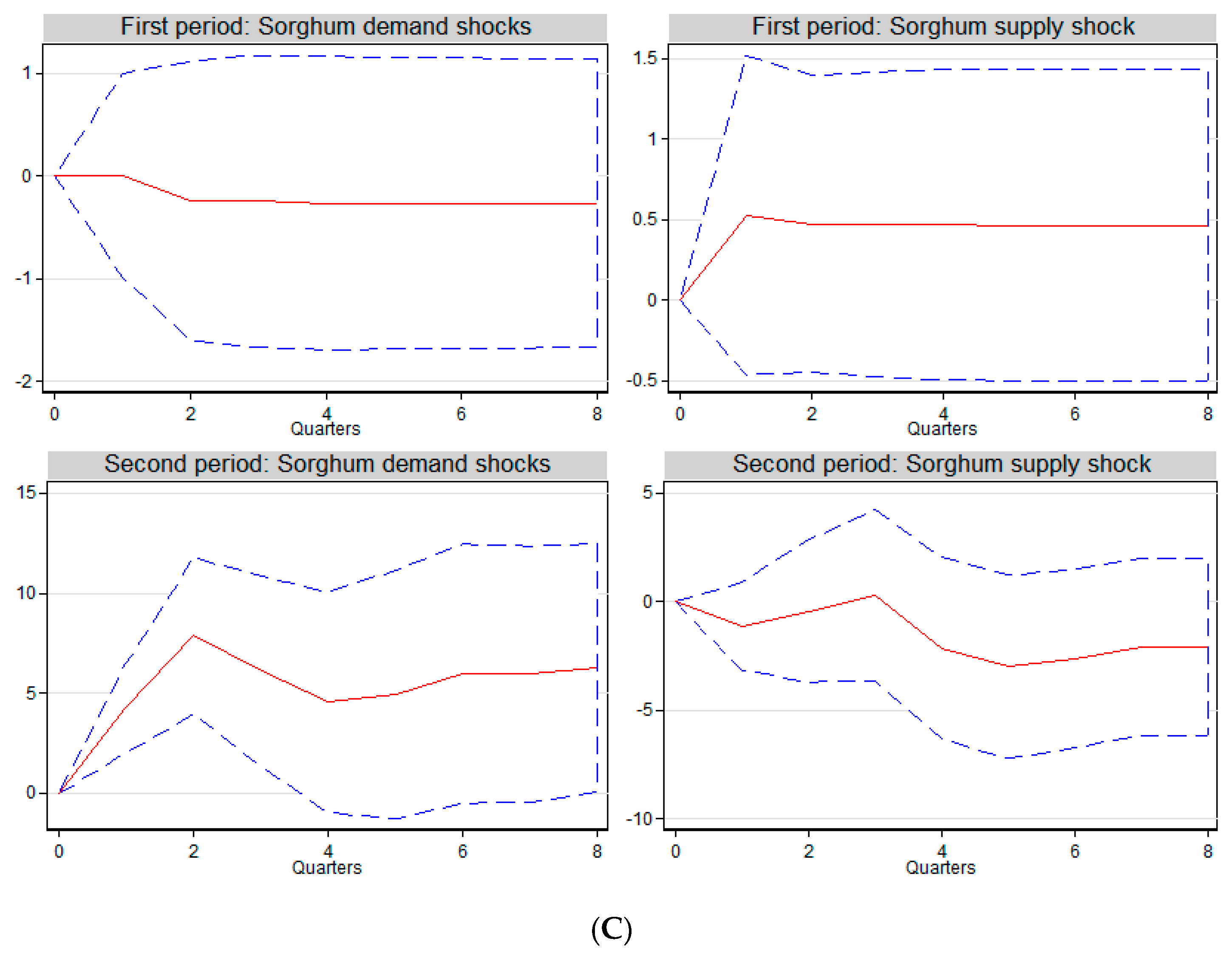
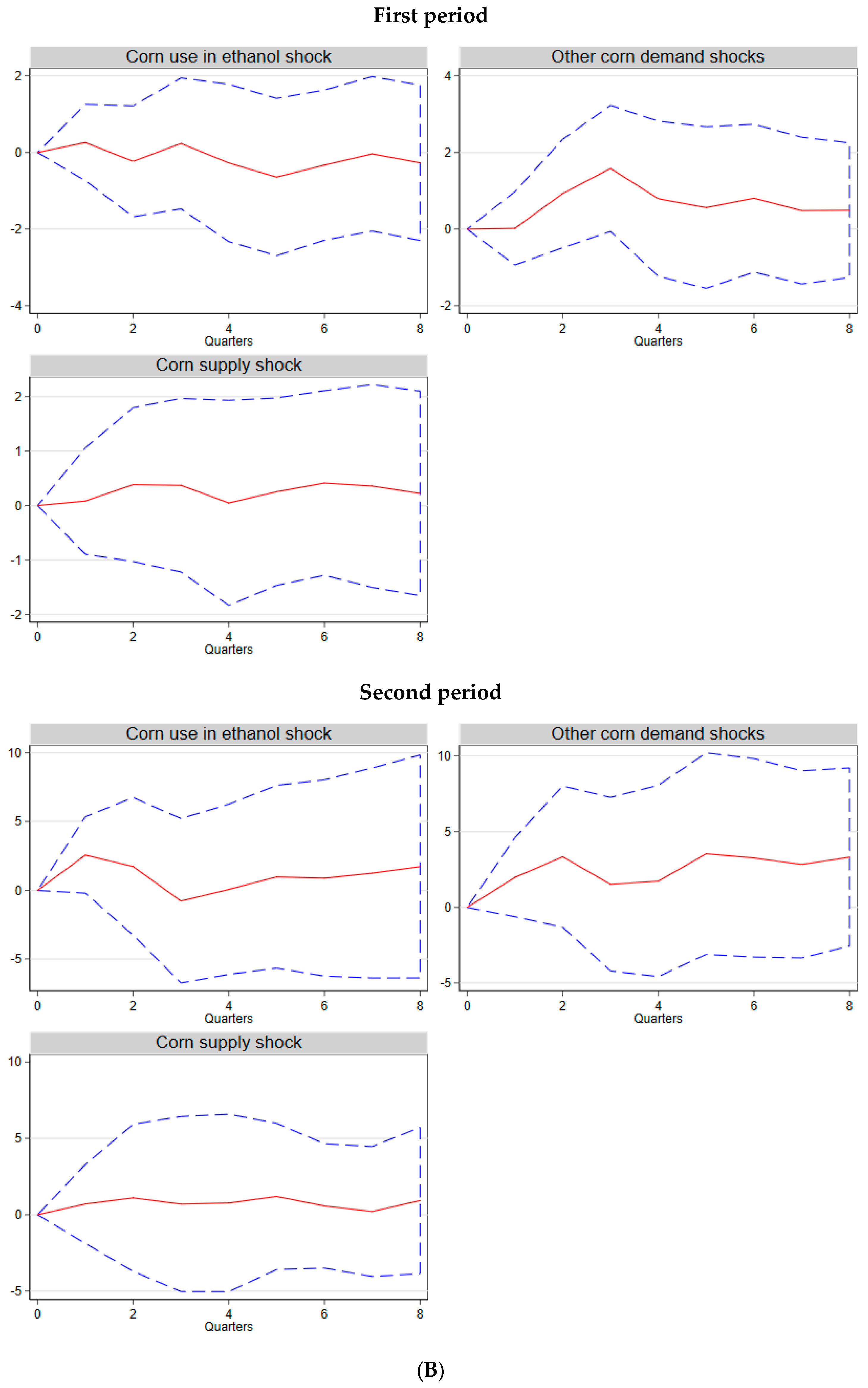
After the Energy Act 2005 by the US Government, the expansion in ethanol production has led to an increase in corn demand, besides the demand from the animal feed industry and human consumption. Therefore, we decided to further decompose corn demand shocks into corn use in ethanol and other corn demand shocks, using the following model, in the period 1986Q1 to 2005Q3 and period 2005Q4 to 2017Q3 (corn marketing year):
The consideration of the Akaike information criterion suggests four lags for this model. Figure 4A,B shows the response of corn use in ethanol to oil price changes and the response of crude oil price to corn-related shocks after decomposing corn demand shocks into corn use in ethanol and other corn demand shocks. According to Figure 4A, oil price did not have a significant impact on corn use in ethanol during the first period. However, the response of corn use in ethanol to oil price variance became significant during the second period. The results suggest that the increase in oil price has created an incentive for more ethanol consumption, which ultimately transfers into the increase in the quantity of corn use in ethanol. On the other hand, such phenomena can only be observed during the second period, when the biofuel mandate became effectively implemented. The timing suggests that the biofuel mandate was successful in inducing consumers to increase biofuel consumption when oil prices increased.
Table 3 shows that the null hypothesis that crude oil price does not Granger-causes corn use in ethanol cannot be rejected during the first period. However, the null is rejected at 5% during the second period. The results suggest that during this period, surges in oil price tended to make biofuel a more viable alternative to fossil fuel, which increased corn demand for ethanol production.
Regarding the responses of crude oil price, Figure 4B shows that agricultural shocks did not have a significant impact on crude oil price during the first period. The situation changed during the second period, when corn use in ethanol shock could trigger a marginally significant response of oil price. The impacts of other corn demand shocks and corn supply shock were insignificant in the second quarter. In Table 3, corn use in ethanol, other corn demand, and corn supply do not Granger-cause crude oil price during the second period.
5.4. The Contribution of Agricultural Shocks to Oil Price Changes
Table 4 quantifies the contribution of oil and corn-related shocks on crude oil price changes, using the method of forecasting error variance decomposition. We can see that other oil-specific demand shocks contributed the most, while the contribution of corn-related shocks was negligible during the first period. During the second period, even though other oil-specific demand shocks still contributed the most to oil price changes, its contribution reduced significantly. In contrast, the contribution of corn demand shocks increased almost fourfold, which contributed 18% to oil price variance and its contribution is comparable to the contribution of the aggregate demand during the second period. In general, the results suggest that corn demand shocks played a larger role in explaining oil price fluctuations, compared to the corn supply shock.
Table 5 shows the contribution of corn-related shocks after decomposing corn demand shocks into corn use in ethanol and other shocks. We can see that corn supply shock was the least important one among corn-related shocks during both periods. In the first period, we can see that other corn demand shocks contributed the most among corn-related shocks. However, during the second period, corn use in ethanol explained almost 10% of oil price changes and became the most important source of shocks among corn-related shocks. The results suggest that the transmission from the corn market to crude oil price is more likely to be explained by the direct biofuel channel than the indirect input cost channel during the second period.
5.5. The Impact of Corn Use in Ethanol on Corn Price and Corn Supply
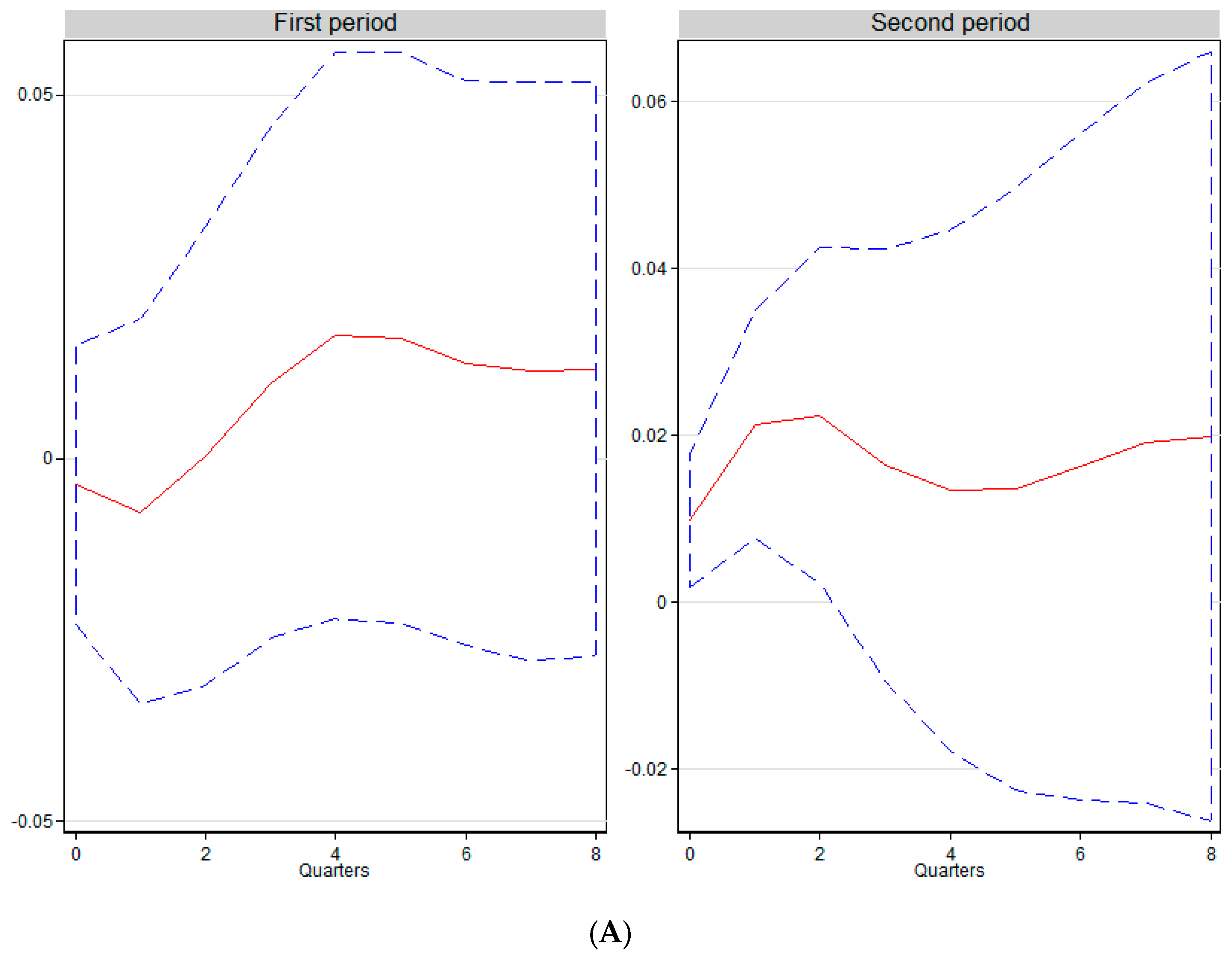
Regarding the food versus fuel literature, various studies have found evidence that the expansion of biofuel may have a negative impact on food security and the welfare of the poor. In this study, Figure 5 shows the responses of corn price and corn supply to changes in corn use in ethanol.
During the first period, the response of corn supply to positive changes in corn use in ethanol was insignificant, while the response of corn price was significantly negative. The negative relationship between corn use in ethanol and corn price is more likely to reflect that corn use in ethanol might react to the future expectation of corn price fluctuation. In particular, the future expectation of a corn price increase may reduce the demand for corn use in ethanol.
During the second period, we can see that the response of corn price to positive shock on corn use in ethanol shock was insignificant. On the other hand, Figure 5 shows that increase in corn use in ethanol can trigger a positive response of corn supply. In general, the results show that corn use in ethanol had a limited impact on corn price during the second period. The reason for this might be that the increase in corn demand for ethanol triggered the expansion of corn production, which neutralized the pressure on corn price.
5.6. Discussions
According to our results, there is a causality running from corn and sorghum prices to oil price and vice versa. The outcomes support the bidirectional relationship between agricultural commodities employed in biofuel production and crude oil price, as suggested by Su et al. (2019). On the other hand, our paper cannot find any correlation between barley and crude oil price, which supports the neutrality of agricultural commodity price to crude oil price changes (Nazlioglu and Soytas 2011, 2012; Ma et al. 2016; Fowowe 2016).
This study found evidence of causality running from the agricultural market to oil prices, which cannot be observed in some previous studies. A possible explanation is that the expansion of biofuel and the agricultural market has not been sufficiently significant to be observable during the sample periods in previous literature. As oil is a major market that is the fundamental driver of almost every sector in the economy, the biofuel and agricultural markets need to develop to a certain size to exert a significant impact on oil prices. On the other hand, the neutral relationship between barley price and oil price could be because barley is not directly related to biofuel production.
However, the story turns out a little different when the agricultural commodity price shocks are separated into supply and demand shocks. For the corn and sorghum case, we observed that agricultural demand shocks are mainly responsible for the impacts of the agricultural markets on the oil market. The outcomes suggest that the increases in agricultural demand have a positive impact on fuel demand. The reason for this might be the indirect input channel, as suggested by Ciaian and Kancs (2011). The input channel suggests that the agricultural markets have become more dependent on the fuel market, because crude oil price can have an impact on fertilizer and transportation costs. Another reason might be the direct biofuel channel, where the increase in biofuel production may add to the agricultural demand, which in return strengthens the increase in fuel demand and oil price (Ciaian 2011; Su et al. 2019).
For the barley case, even though the barley price was not a Granger cause for oil price, we observed that the response of oil price to barley supply shock was significant during the second period. The results support the hypothesis that when barley demand is inelastic, the productivity shock in the barley market may create an oversupply situation, which reduces the agricultural demand and therefore fuel demand (Ciaian 2011).
In general, our results confirm that both supply and demand shocks in the agricultural markets can lead to fluctuation in the crude oil market. We also confirmed that crude oil price can have a great impact on corn use in ethanol. The results support the hypothesis that the ethanol market is dependent on crude oil price (Chen and Saghaian 2015). On the other hand, corn use in ethanol can also cause crude oil prices in the second period. This outcome is in accordance with the direct biofuel channel that ethanol production expansion can increase fuel demand in the corn sector. Regarding the biofuel channel, Ciaian and Kancs (2011) argued that bio-ethanol production can impact crude oil price in two opposite directions. Firstly, an increase in corn demand due to biofuel production may increase the supply for corn. The increase in agricultural production due to an increase in corn demand may lead to the increase in oil demand. As result, an increase in corn demand due to bioethanol expansion will eventually lead to an increase in oil price, because of the rise in fuel demand. Secondly, biofuel production increases the total energy supply and, therefore, reduces oil price. Our empirical results show that an increase in corn use in ethanol can have a positive impact on both corn supply and oil price. Therefore, our study supports the hypothesis that bioethanol expansion may increase the dependency of the economy on fossil fuels.
Regarding the food versus fuel literature, our results show that an increase in corn use in ethanol cannot impact corn price, which contrasts with previous literature (Hao et al. 2017; Apergis et al. 2017; Chiu et al. 2016). On the other hand, we observed that an increase in corn use in ethanol can increase corn supply. This outcome partly explains why corn use in ethanol cannot impact corn price. Our results support the hypothesis that the expansion of biofuel production has greatly attracted farming resources to corn production (Büyüktahtakın and Cobuloglu 2015; De Martino Jannuzzi 1991; Fradj and Jayet 2016; Herrmann et al. 2017).
It was shown in the preliminary analysis that corn supply has increased significantly, while the other agricultural commodity supplies decreased dramatically during the second period. The expansion of corn and the shrinking of other agricultural commodity supplies happened during the same period as the expansion of biofuel production. These outcomes suggest that the expansion of biofuel production in recent years has caused the land use management to be shifted against the production of food crops. The increase in biofuel demand led to the expansion of certain agricultural commodities which are feedstocks of biofuel production. As agricultural resources are limited, the expansion of these crops may lead to the reduction of farming areas and other agricultural resources invested in other agricultural commodity productions, which creates supply disruptions and, finally, increases of several agricultural commodity prices. However, there should be more research in this direction before we can reach any conclusion. Future research should focus on the impact of corn production expansion on the supplies of non-biofuel agricultural commodities and their prices to validate the hypothesis.
In general, we observed that the effects of agricultural shocks only happened during the second period. However, the energy act is unlikely to be fully responsible for causing the agricultural shocks, as other major economic events happened in the same period, such as the global financial crisis, the food crisis, or even climate change. Therefore, a future study should investigate other sub-periods to identify the timeline of those shocks.
On the other hand, as biofuel enhancement continues in the future, it is likely to attract many real economic resources, which may have many drawbacks. Firstly, even though the initial objective of biofuel is to increase the energy supply and replace fossil fuel, the current farming machinery is still dependent on oil. Thus, to make biofuel more sustainable, future machinery needs to be more compatible with the use of biofuel. Secondly, growing more energy crops means that more non-arable land will be turn into arable land, which is costly to the environment. Lastly, as the profits of biofuel production increase, farmers will have more incentive to substitute food crops with energy crops, which will have negative effects on food security. These sources of drawbacks need to be dealt with to improve the long-term effectiveness of biofuel enhancement.
6. Concluding Remarks
This study investigated the impact of agricultural shocks in the period from 1986m1 to 2018m5 using the SVAR model. Our sample data was divided into two subsamples: 1986m1–2005m12 and 2006m1–2018m5. The paper found that agricultural shocks had an effect on oil price during the second period. The findings are consistent with the theoretical model that agricultural shocks can influence crude oil price through the indirect cost-push effect and direct biofuel channel. Furthermore, we decomposed the agricultural commodity price shocks into agricultural supply and demand shocks. The demand shocks were later separated into corn use in ethanol and other corn demand shocks. The outcomes from the impulse response function suggest that different agricultural shocks can have different effects on oil price. Firstly, positive agricultural supply shocks can have a negative impact on oil price due to the reduction in fuel demand. Secondly, agricultural demand shocks can have a positive effect on oil price, especially corn use in ethanol.
In particular, we could not find any significant response of the crude oil price to the agricultural shocks during the first period. However, the situation changed sharply during the second period, when agricultural shocks triggered a significant response in oil price. On the other hand, not every agricultural shock can have a significant impact on oil price. While oil price does not respond significantly to the shocks to the corn and sorghum supplies, the response of crude oil price to barley supply shock was significant during the second period. On the other hand, corn and sorghum demand shocks triggered a significant response in oil price in the second period.
We used the variance decomposition to quantify the contribution of agricultural demand shocks on oil price variations. The outcomes suggest that corn use in ethanol played an important role in the impact of corn demand shocks on oil price during the second period. The results support the direct biofuel channel, which suggests that the expansion of bio-energy production has made oil price vulnerable to corn demand shocks.
Overall, the paper’s findings suggest that the links between agricultural market and oil prices have been strengthened since the issue of the Energy Policy Act of 2005. During this period, Table 6 shows that oil prices can influence agricultural prices, such as corn and sorghum prices, and increase the demand for corn use in ethanol. Oil prices also respond to shocks on agricultural supply, agricultural demand, and corn use in ethanol. In particular, the productivity shocks on barley supply can have a negative effect on oil prices. In corn and sorghum cases, agricultural demand shocks can have a positive impact on oil price. Moreover, corn use in ethanol plays an important role in the system, as the expansion of corn use in ethanol incentivizes growing more corn and increases the demand for oil in the agricultural sector. These findings are interesting because they show that biofuel expansion and an increase in size of the agricultural sector have become sufficiently significant to influence oil prices, which are the fundamental drivers for all sectors of the economy.
The policymakers in the agricultural and energy sectors can benefit from the findings of this paper. Firstly, the original purpose of the increase in bio-ethanol production is to reduce the dependency of the economy on fossil fuel. However, this strategy may have backfired because the increase in corn production due to the expansion of corn use in ethanol has led to a rise in fuel demand. Secondly, our results indicate that farmers have reacted to the rise in corn demand and increased the corn supply. Their decisions can affect the investment in growing other agricultural commodities, because agricultural resources such as land and water are limited. It will be interesting to study whether the increasing corn supply due to the expansion of corn use in ethanol can have an impact on the supplies and prices of other important agricultural commodities.
Author Contributions
Conceptualization, T.N.V.; methodology, D.H.V.; software, C.M.H.; formal analysis, T.N.V.; investigation, L.T.-H.V.; resources, C.M.H.; data curation, T.N.V., C.M.H. and L.T.-H.V.; writing—original draft preparation, T.N.V. and L.T.-H.V.; writing—review and editing, D.H.V.
Funding
This research was funded by Ho Chi Minh City Open University grant number E2019.05.2.
Acknowledgments
We are grateful to the three anonymous referees for their constructive comments. We also thank the participants at the 3rd Vietnam’s Business and Economics Research Conference VBER2019 (Ho Chi Minh City Open University, Vietnam, 18–20 July 2019) for their helpful suggestions. The authors wish to acknowledge financial supports from Ho Chi Minh City Open University. The authors are solely responsible for any remaining errors or shortcomings.
Conflicts of Interest
The authors declare no conflicts of interest.
References
- Adam, Pasrun, La Ode Saidi, La Tondi, La Ode, and Arsad Sani. 2018. The Causal Relationship between Crude Oil Price, Exchange Rate and Rice Price. International Journal of Energy Economics and Policy 8: 90–94. [Google Scholar]
- Ahmadi, Maryam, Niaz Bashiri Behmiri, and Matteo Manera. 2016. How Is Volatility in Commodity Markets Linked to Oil Price Shocks? Energy Economics 59: 11–23. [Google Scholar] [CrossRef]
- Allen, David E., Chialin Chang, Michael McAleer, and Abhay K Singh. 2018. A Cointegration Analysis of Agricultural, Energy and Bio-Fuel Spot, and Futures Prices. Applied Economics 50: 804–23. [Google Scholar] [CrossRef]
- Apergis, Nicholas, Sofia Eleftheriou, and Dimitrios Voliotis. 2017. Asymmetric Spillover Effects between Agricultural Commodity Prices and Biofuel Energy Prices. International Journal of Energy Economics and Policy 7: 166–77. [Google Scholar]
- Avalos, Fernando. 2014. Do Oil Prices Drive Food Prices? The Tale of a Structural Break. Journal of International Money and Finance 42: 253–71. [Google Scholar] [CrossRef]
- Baumeister, Christiane, and Lutz Kilian. 2014. Do Oil Price Increases Cause Higher Food Prices? Economic Policy 29: 691–747. [Google Scholar] [CrossRef]
- Baumeister, Christiane, and Lutz Kilian. 2016. Understanding the Decline in the Price of Oil since June 2014. Journal of the Association of Environmental and Resource Economists 3: 131–58. [Google Scholar] [CrossRef]
- Bayramoğlu, Arzu Tay, Murat Çetin, and Gökhan Karabulut. 2016. The Impact of Biofuels Demand on Agricultural Commodity Prices: Evidence from US Corn Marketi&ii. Journal of Economics 4: 189–206. [Google Scholar]
- Bentivoglio, Deborah, Adele Finco, and Mirian Bacchi. 2016. Interdependencies between Biofuel, Fuel and Food Prices: The Case of the Brazilian Ethanol Market. Energies 9: 464. [Google Scholar] [CrossRef]
- Büyüktahtakın, Esra, and Halil I Cobuloglu. 2015. Food vs. Biofuel: An Optimization Approach to the Spatio-Temporal Analysis of Land-Use Competition and Environmental Impacts. Applied Energy 140: 418–34. [Google Scholar] [CrossRef]
- Chang, Chia-lin, Michael Mcaleer, and Yu-ann Wang. 2018. Modelling Volatility Spillovers for Bio-Ethanol, Sugarcane and Corn Spot and Futures Prices. Renewable and Sustainable Energy Reviews 81: 1002–18. [Google Scholar] [CrossRef]
- Chen, Bo, and Sayed Saghaian. 2015. The Relationship among Ethanol, Sugar and Oil Prices in Brazil: Cointegration Analysis with Structural Breaks. Paper presented at the 2015 Annual Meeting, Atlanta, GA, USA, January 31–February 3. [Google Scholar]
- Chiu, Fan Ping, Chia Sheng Hsu, Alan Ho, and Chi Chung Chen. 2016. Modeling the Price Relationships between Crude Oil, Energy Crops and Biofuels. Energy 109: 845–57. [Google Scholar] [CrossRef]
- Ciaian, Pavel. 2011. Food, Energy and Environment: Is Bioenergy the Missing Link? Food Policy 36: 571–80. [Google Scholar] [CrossRef]
- Ciaian, Pavel, and d’Artis Kancs. 2011. Interdependencies in the Energy-Bioenergy-Food Price Systems: A Cointegration Analysis. Resource and Energy Economics 33: 326–48. [Google Scholar] [CrossRef]
- Clemente, Jesus, Antonio Montañés, and Marcelo Reyes. 1998. Testing for a Unit Root in Variables with a Double Change in the Mean. Economics Letters 59: 175–82. [Google Scholar] [CrossRef]
- Cooley, Thomas F., and Stephen F. LeRoy. 1985. Atheoretical Macroeconometrics: A Critique. Journal of Monetary Economics 16: 283–308. [Google Scholar] [CrossRef]
- De Gorter, Harry, Dusan Drabik, and David R. Just. 2013. Biofuel Policies and Food Grain Commodity Prices 2006–2012: All Boom and No Bust? AgBioForum 16: 1–13. [Google Scholar]
- De Martino Jannuzzi, Gilberto. 1991. Competition between Energy and Agricultural Production: A Discussion of a Country’s Best Strategies. Energy Economics 13: 199–202. [Google Scholar] [CrossRef]
- Dickey, David A., and Wayne A. Fuller. 1979. Distribution of the Estimators for Autoregressive Time Series with a Unit Root. Journal of the American Statistical Association 74: 427–31. [Google Scholar]
- Dutta, Anupam. 2018. Cointegration and Nonlinear Causality among Ethanol-related Prices: Evidence from Brazil. GCB Bioenergy 10: 335–42. [Google Scholar] [CrossRef]
- Dutta, Anupam, Juha Junttila, and Gazi Salah. 2018. Does Corn Market Uncertainty Impact the US Ethanol Prices? GCB Bioenergy 10: 683–93. [Google Scholar] [CrossRef]
- Enciso, Sergio René Araujo, Thomas Fellmann, Ignacio Pérez Dominguez, and Fabien Santini. 2016. Abolishing Biofuel Policies: Possible Impacts on Agricultural Price Levels, Price Variability and Global Food Security. Food Policy 61: 9–26. [Google Scholar] [CrossRef]
- Fowowe, Babajide. 2016. Do Oil Prices Drive Agricultural Commodity Prices? Evidence from South Africa. Energy 104: 149–57. [Google Scholar] [CrossRef]
- Fradj, N. Ben, and P. A. Jayet. 2016. Land Use Policy Competition between Food, Feed, and (Bio) Fuel: A Supply-Side Model Based Assessment at the European Scale. Land Use Policy 52: 195–205. [Google Scholar] [CrossRef]
- Han, Liyan, Yimin Zhou, and Libo Yin. 2015. Exogenous Impacts on the Links between Energy and Agricultural Commodity Markets. Energy Economics 49: 350–58. [Google Scholar] [CrossRef]
- Hao, Na, Peter Pedroni, Gregory Colson, and Michael Wetzstein. 2017. The Linkage between the US Ethanol Market and Developing Countries’ Maize Prices: A Panel SVAR Analysis. Agricultural Economics 48: 629–38. [Google Scholar] [CrossRef]
- Herrmann, Raoul, Charles Jumbe, Michael Bruentrup, and Evans Osabuohien. 2017. Competition between Biofuel Feedstock and Food Production: Empirical Evidence from Sugarcane Outgrower Settings in Malawi. Biomass and Bioenergy. [Google Scholar] [CrossRef]
- Jha, Shikha, and P. V. Srinivasan. 2001. Food Inventory Policies under Liberalized Trade. International Journal of Production Economics 71: 21–29. [Google Scholar] [CrossRef]
- Kilian, Lutz. 2009. Not All Oil Price Shocks Are Alike: Disentangling Demand and Supply Shocks in the Crude Oil Market. American Economic Review 99: 1053–69. [Google Scholar] [CrossRef]
- Kilian, Lutz. 2018. Measuring Global Economic Activity: Reply. pp. 1–5. Available online: https://sites.google.com/site/lkilian2019/research/data-sets (accessed on 15 March 2019).
- Koirala, Krishna H., Ashok K. Mishra, Jeremy M. D. Antoni, and Joey E. Mehlhorn. 2015. Energy Prices and Agricultural Commodity Prices: Testing Correlation Using Copulas Method. Energy 81: 430–36. [Google Scholar] [CrossRef]
- Kristoufek, Ladislav, Karel Janda, and David Zilberman. 2016. Comovements of Ethanol-related Prices: Evidence from Brazil and the USA. Gcb Bioenergy 8: 346–56. [Google Scholar] [CrossRef]
- Kwiatkowski, Denis, Peter C. B. Phillips, Peter Schmidt, and Yongcheol Shin. 1992. Testing the Null Hypothesis of Stationarity against the Alternative of a Unit Root: How Sure Are We That Economic Time Series Have a Unit Root? Journal of Econometrics 54: 159–78. [Google Scholar] [CrossRef]
- Lee, Junsoo, and Mark C. Strazicich. 2003. Minimum Lagrange Multiplier Unit Root Test with Two Structural Breaks. Review of Economics and Statistics 85: 1082–89. [Google Scholar] [CrossRef]
- Lucotte, Yannick. 2016. Co-Movements between Crude Oil and Food Prices: A Post-Commodity Boom Perspective. Economics Letters 147: 142–47. [Google Scholar] [CrossRef]
- Lumsdaine, Robin L., and David H. Papell. 1997. Multiple Trend Breaks and the Unit-Root Hypothesis. Review of Economics and Statistics 79: 212–18. [Google Scholar] [CrossRef]
- Ma, Z., R. Xu, and X. Dong. 2016. World Oil Prices and Agricultural Commodity Prices: The Evidence from China. Agricultural Economics (Zemědělská Ekonomika) 61: 564–76. [Google Scholar] [CrossRef]
- Mcphail, Lihong Lu. 2011. Assessing the Impact of US Ethanol on Fossil Fuel Markets: A Structural VAR Approach. Energy Economics 33: 1177–85. [Google Scholar] [CrossRef]
- McPhail, Lihong Lu, Xiaodong Du, and Andrew Muhammad. 2012. Disentangling Corn Price Volatility: The Role of Global Demand, Speculation, and Energy. Journal of Agricultural & Applied Economics 44: 401–10. [Google Scholar] [CrossRef]
- Natanelov, Valeri, Mohammad J. Alam, Andrew M. McKenzie, and Guido Van Huylenbroeck. 2011. Is There Co-Movement of Agricultural Commodities Futures Prices and Crude Oil? Energy Policy 39: 4971–84. [Google Scholar] [CrossRef]
- Nazlioglu, Saban, and Ugur Soytas. 2011. World Oil Prices and Agricultural Commodity Prices: Evidence from an Emerging Market. Energy Economics 33: 488–96. [Google Scholar] [CrossRef]
- Nazlioglu, Saban, and Ugur Soytas. 2012. Oil Price, Agricultural Commodity Prices, and the Dollar: A Panel Cointegration and Causality Analysis. Energy Economics 34: 1098–104. [Google Scholar] [CrossRef]
- Nguyen, Van Phuc, and Duc Hong Vo. 2019. Macroeconomics Determinants of Exchange Rate Pass-Through: New Evidence from the Asia-Pacific Region. Emerging Markets Finance and Trade. [Google Scholar] [CrossRef]
- Perron, Pierre. 1989. The Great Crash, the Oil Price Shock, and the Unit Root Hypothesis. Econometrica: Journal of the Econometric Society 57: 1361–401. [Google Scholar] [CrossRef]
- Perron, Pierre, and Timothy J. Vogelsang. 1992. Nonstationarity and Level Shifts with an Application to Purchasing Power Parity. Journal of Business & Economic Statistics 10: 301–20. [Google Scholar]
- Persson, U. Martin. 2015. The Impact of Biofuel Demand on Agricultural Commodity Prices: A Systematic Review. Wiley Interdisciplinary Reviews: Energy and Environment 4: 410–28. [Google Scholar] [CrossRef]
- Phillips, Peter C. B., and Pierre Perron. 1988. Testing for a Unit Root in Time Series Regression. Biometrika 75: 335–46. [Google Scholar] [CrossRef]
- Qiu, Cheng, Gregory Colson, Cesar Escalante, and Michael Wetzstein. 2012. Considering Macroeconomic Indicators in the Food before Fuel Nexus. Energy Economics 34: 2021–28. [Google Scholar] [CrossRef]
- Saghaian, Sayed, Mehdi Nemati, Cory Walters, and Bo Chen. 2018. Asymmetric Price Volatility Transmission between US Biofuel, Corn, and Oil Markets. Journal of Agricultural and Resource Economics 43: 46. [Google Scholar]
- Serra, Teresa, and David Zilberman. 2013. Biofuel-Related Price Transmission Literature: A Review. Energy Economics 37: 141–51. [Google Scholar] [CrossRef]
- Su, Chi Wei, Xiao-Qing Wang, Ran Tao, and Oana-Ramona LobonŢ. 2019. Do Oil Prices Drive Agricultural Commodity Prices? Further Evidence in a Global Bio-Energy Context. Energy 172: 691–701. [Google Scholar] [CrossRef]
- To, Anh, Dao Ha, Ha Nguyen, and Duc Vo. 2019. The Impact of Foreign Direct Investment on Environment Degradation: Evidence from Emerging Markets in Asia. International Journal of Environmental Research and Public Health 16: 1636. [Google Scholar] [CrossRef] [PubMed]
- To, Hang, and R. Quentin Grafton. 2015. Oil Prices, Biofuels Production and Food Security: Past Trends and Future Challenges. Food Security 7: 323–36. [Google Scholar] [CrossRef]
- Vacha, Lukas, Karel Janda, Ladislav Kristoufek, and David Zilberman. 2013. Time–Frequency Dynamics of Biofuel–Fuel–Food System. Energy Economics 40: 233–41. [Google Scholar] [CrossRef]
- Vo, Duc, Tan Vu, Anh Vo, and Michael McAleer. 2019. Modeling the Relationship between Crude Oil and Agricultural Commodity Prices. Energies 12: 1344. [Google Scholar] [CrossRef]
- Vo, Anh, Quan Le, Phuc Nguyen, Chi Ho, and Duc Vo. 2018. Exchange Rate Pass-Through in ASEAN Countries: An Application of the SVAR Model. Emerging Markets Finance and Trade. [Google Scholar] [CrossRef]
- Wang, Yudong, Chongfeng Wu, and Li Yang. 2014. Oil Price Shocks and Agricultural Commodity Prices. Energy Economics 44: 22–35. [Google Scholar] [CrossRef]
- Zafeiriou, Eleni, Garyfallos Arabatzis, Paraskevi Karanikola, Stilianos Tampakis, and Stavros Tsiantikoudis. 2018. Agricultural Commodity and Crude Oil Prices: An Empirical Investigation of Their Relationship. Sustainability 10: 1199. [Google Scholar] [CrossRef]
- Zhang, Zibin, Luanne Lohr, Cesar Escalante, and Michael Wetzstein. 2010. Food versus Fuel: What Do Prices Tell Us? Energy Policy 38: 445–51. [Google Scholar] [CrossRef]
- Zhou, Wei, and Bruce A. Babcock. 2017. Using the Competitive Storage Model to Estimate the Impact of Ethanol and Fueling Investment on Corn Prices. Energy Economics 62: 195–203. [Google Scholar] [CrossRef]
- Zivot, Eric, and Donald W. K. Andrews. 2002. Further Evidence on the Great Crash, the Oil-Price Shock, and the Unit-Root Hypothesis. Journal of Business & Economic Statistics 20: 25–44. [Google Scholar]
| 1 | The data can be obtained from the following website: https://sites.google.com/site/lkilian2019/research/data-sets. |
| 2 | The results of the stability tests are available upon request. |
Figure 1.
(A) Response of agricultural commodity prices to oil-specific demand shocks; (B) response of oil price to agricultural related-shocks. Notes: Red lines represent cumulative orthogonalized impulse–response functions while blue lines represent 95% confidence intervals.
Figure 1.
(A) Response of agricultural commodity prices to oil-specific demand shocks; (B) response of oil price to agricultural related-shocks. Notes: Red lines represent cumulative orthogonalized impulse–response functions while blue lines represent 95% confidence intervals.


Figure 2.
(A) Response of barley price to barley-related shocks. (B) Response of corn price to corn-related shocks. (C) Response of sorghum price to sorghum-related shocks. Notes: Red lines represent cumulative orthogonalized impulse–response functions while blue lines represent 95% confidence intervals.


Figure 3.
(A) Response of oil price to barley supply and demand shocks. (B) Response of oil price to corn supply and demand shocks. (C) Response of oil price to sorghum supply and demand shocks. Notes: Red lines represent cumulative orthogonalized impulse–response functions while blue lines represent 95% confidence intervals.


Figure 4.
(A) Response of corn use in ethanol to oil price shocks. (B) Response of oil price to corn-related shocks. Notes: Red lines represent cumulative orthogonalized impulse–response functions while blue lines represent 95% confidence intervals.
Figure 4.
(A) Response of corn use in ethanol to oil price shocks. (B) Response of oil price to corn-related shocks. Notes: Red lines represent cumulative orthogonalized impulse–response functions while blue lines represent 95% confidence intervals.


Figure 5.
Response of corn supply and corn price to corn use in ethanol shocks. Notes: Red lines represent cumulative orthogonalized impulse–response functions while blue lines represent 95% confidence intervals.
Figure 5.
Response of corn supply and corn price to corn use in ethanol shocks. Notes: Red lines represent cumulative orthogonalized impulse–response functions while blue lines represent 95% confidence intervals.


Table 1.
Data Description.
| January 1986–December 2005 | ||||||
| Variable | Mean | SD | Max | Min | Skewness | Kurtosis |
| Oil supply | 11.06 | 0.08 | 11.22 | 10.90 | 0.14 | 2.14 |
| Kilian index | −0.98 | 41.72 | 125.00 | −81.10 | 1.08 | 4.34 |
| Oil price | 34.85 | 10.32 | 75.68 | 14.45 | 1.30 | 5.70 |
| Barley price | 3.58 | 0.70 | 5.97 | 2.43 | 1.28 | 4.60 |
| Corn price | 3.59 | 0.91 | 6.69 | 2.09 | 0.67 | 3.26 |
| Sorghum price | 3.33 | 0.85 | 6.49 | 1.89 | 0.72 | 3.63 |
| Barley supply | 366.48 | 169.31 | 937.11 | 125.11 | 1.10 | 4.07 |
| Corn supply | 6924.41 | 2908.72 | 13,228.27 | 1720.75 | 0.22 | 2.06 |
| Sorghum supply | 484.69 | 350.66 | 1489.88 | 70.39 | 1.01 | 3.34 |
| Biofuel demand | 4.85 | 0.48 | 5.96 | 4.12 | 0.67 | 2.62 |
| January 2006–May 2018 | ||||||
| Variable | Mean | SD | Max | Min | Skewness | Kurtosis |
| Oil supply | 11.25 | 0.04 | 11.32 | 11.19 | 0.40 | 1.72 |
| Kilian index | 3.23 | 79.92 | 188.00 | −164.00 | 0.58 | 2.57 |
| Oil price | 81.73 | 27.55 | 147.58 | 28.39 | 0.05 | 2.02 |
| Barley price | 5.03 | 0.93 | 6.78 | 2.94 | −0.19 | 2.36 |
| Corn price | 4.45 | 1.38 | 7.87 | 2.38 | 0.78 | 2.46 |
| Sorghum price | 4.28 | 1.32 | 7.12 | 2.10 | 0.63 | 2.25 |
| Barley supply | 199.79 | 61.10 | 321.26 | 98.99 | 0.46 | 2.11 |
| Corn supply | 8999.50 | 4061.65 | 16,908.16 | 2805.80 | 0.27 | 1.93 |
| Sorghum supply | 226.60 | 144.28 | 618.76 | 34.33 | 0.94 | 3.09 |
| Biofuel demand | 6.97 | 0.34 | 7.26 | 6.01 | −1.54 | 4.19 |
Table 2.
(A) Unit root tests without structural break. (B) Unit root test with a structural break.
| (A) | ||||||
| ADF | PP | KPSS | ||||
| Variables | Original Series | First Order Difference | Original Series | First Order Difference | Original Series | First Order Difference |
| Oil production | −0.42 | −6.75 *** | −1.07 | −21.32 *** | 0.14 * | 0.03 |
| Kilian index | −2.69 * | −7.03 *** | −3.02 ** | −14.21 *** | 0.26 *** | 0.03 |
| Oil price | −1.78 | −9.7 *** | −2.18 | −11.11 *** | 0.21 ** | 0.07 |
| Barley price | −2.24 | −10.95 *** | −2.27 | −20.08 *** | 0.3 *** | 0.05 |
| Corn price | −2.94 ** | −5.34 *** | −2.72 * | −12.57 *** | 0.2 ** | 0.05 |
| Sorghum price | −2.56 | −8.12 *** | −2.94 ** | −14.63 *** | 0.18 ** | 0.04 |
| Barley supply | −4.12 *** | −4.58 *** | −5.96 *** | −25.4 *** | 0.35 *** | 0.02 |
| Corn supply | −1.97 | −5.71 *** | −11.15 *** | −25.19 *** | 0.22 *** | 0.02 |
| Sorghum supply | −3.19 *** | −4.94 *** | −5.94 *** | −24.57 *** | 0.42 *** | 0.02 |
| Bio demand | −0.36 | −4.43 *** | −0.19 | −10.27 *** | 0.37 *** | 0.16 ** |
| (B) | ||||||
| Model A1: Breaks in Intercept | Model A2: Breaks in Trend | Model A3: Breaks in Intercept and Trend | ||||
| Variables | Original Series | First Order Difference | Original Series | First Order Difference | Original Series | First Order Difference |
| Oil production | −5.96 *** | −11.16 *** | −5.49 *** | −11.08 *** | −5.95 *** | −11.15 *** |
| Kilian index | −4.29 | −11.51 *** | −3.6 | −11.34 *** | −4.71 | −11.69 *** |
| Oil price | −4.86 ** | −10.05 *** | −4.1 | −9.66 *** | −5.15 ** | −10.03 *** |
| Barley price | −4.23 | −11.11 *** | −3.03 | −11.02 *** | −4.01 | −11.13 *** |
| Corn price | −4.28 | −12.92 *** | −3.29 | −12.67 *** | −4.64 | −13.06 *** |
| Sorghum price | −4.64 * | −9.04 *** | −3.83 | −8.83 *** | −5.59 ** | −9.22 *** |
| Barley supply | −3.77 | −5.05 ** | −3.18 | −5.67 *** | −3.4 | −5.62 *** |
| Corn supply | −2.36 | −5.27 ** | −2.68 | −5.19 *** | −2.56 | −5.34 ** |
| Sorghum supply | −1.94 | −5.93 *** | −6.78 *** | −5.54 *** | −4.22 | −6.01 *** |
| Bio demand | −3.08 | −6.01 *** | −2.06 | −5.69 *** | −2.43 | −6.12 *** |
Notes: *, **, *** denote significance at the 10%, 5%, 1% level respectively.
Table 3.
Granger causality.
| Direction of Causality | 1986m1–2005m12 | 2006m1–2018m5 |
|---|---|---|
| Oil price → Barley price | 1.32 | 0.90 |
| Barley price → Oil price | 1.45 | 0.20 |
| Oil price → Corn price | 4.56 | 0.01 |
| Corn price → Oil price | 1.42 | 5.97 ** |
| Oil price → Sorghum price | 2.00 | 1.12 |
| Sorghum price → Oil price | 0.59 | 3.27 * |
| Corn demand → Oil price | 3.22 | 11.8 ** |
| Corn supply → Oil price | 1.05 | 1.04 |
| Oil price → Corn use in ethanol | 1.23 | 11.29 ** |
| Corn use in ethanol → Oil price | 6.16 | 6.52 |
Notes: *, ** denote significance at the 10%, 5% level respectively.
Table 4.
Percentage contribution to oil price variation (before the decomposition of corn demand).
| First Period | Second Period | |||||||||
|---|---|---|---|---|---|---|---|---|---|---|
| Quarters | Oil Supply Shock | Aggregate Demand Shock | Other Oil-Demand Shocks | Corn Demand Shocks | Corn Supply Shock | Oil Supply Shock | Aggregate Demand Shock | Other Oil-Demand Shocks | Corn Demand Shocks | Corn Supply Shock |
| 2 | 0.032 | 0.012 | 0.954 | 0.001 | 0.001 | 0.068 | 0.272 | 0.518 | 0.139 | 0.003 |
| 3 | 0.030 | 0.033 | 0.902 | 0.033 | 0.002 | 0.116 | 0.224 | 0.484 | 0.170 | 0.006 |
| 4 | 0.030 | 0.080 | 0.850 | 0.036 | 0.003 | 0.184 | 0.200 | 0.435 | 0.173 | 0.008 |
| 5 | 0.030 | 0.080 | 0.836 | 0.048 | 0.006 | 0.199 | 0.196 | 0.424 | 0.169 | 0.013 |
| 6 | 0.030 | 0.094 | 0.821 | 0.049 | 0.006 | 0.194 | 0.190 | 0.414 | 0.189 | 0.013 |
| 7 | 0.032 | 0.101 | 0.811 | 0.049 | 0.007 | 0.204 | 0.185 | 0.403 | 0.186 | 0.020 |
| 8 | 0.034 | 0.101 | 0.807 | 0.050 | 0.008 | 0.217 | 0.181 | 0.394 | 0.182 | 0.026 |
Table 5.
Percentage contribution to oil price variation (after the decomposition of corn demand).
| First Period | Second Period | |||||||
|---|---|---|---|---|---|---|---|---|
| Quarters | Oil-Related Shocks | Corn Use in Ethanol Shock | Other Corn Demand Shocks | Corn Supply Shock | Oil-Related Shocks | Corn Use in Ethanol Shock | Other Corn Demand Shocks | Corn Supply Shock |
| 2 | 0.996 | 0.003 | 0.000 | 0.000 | 0.917 | 0.049 | 0.030 | 0.004 |
| 3 | 0.943 | 0.015 | 0.038 | 0.005 | 0.900 | 0.053 | 0.042 | 0.005 |
| 4 | 0.921 | 0.022 | 0.053 | 0.004 | 0.846 | 0.089 | 0.060 | 0.005 |
| 5 | 0.884 | 0.032 | 0.076 | 0.008 | 0.846 | 0.091 | 0.058 | 0.005 |
| 6 | 0.877 | 0.037 | 0.077 | 0.010 | 0.824 | 0.093 | 0.077 | 0.006 |
| 7 | 0.872 | 0.040 | 0.077 | 0.011 | 0.823 | 0.092 | 0.076 | 0.008 |
| 8 | 0.866 | 0.043 | 0.081 | 0.011 | 0.822 | 0.092 | 0.077 | 0.009 |
Table 6.
Summary of findings.
| Explanatory Variables | Dependent Variables | ||||
|---|---|---|---|---|---|
| Oil Price | Agricultural Prices | Agricultural Supplies | Agricultural Demand | Corn Use in Ethanol | |
| Oil price | |||||
| Agricultural prices | |||||
| Agricultural supplies | |||||
| Agricultural demand | |||||
| Corn use in ethanol | |||||
© 2019 by the authors. Licensee MDPI, Basel, Switzerland. This article is an open access article distributed under the terms and conditions of the Creative Commons Attribution (CC BY) license (http://creativecommons.org/licenses/by/4.0/).
Share and Cite
MDPI and ACS Style
Vu, T.N.; Vo, D.H.; Ho, C.M.; Van, L.T.-H. Modeling the Impact of Agricultural Shocks on Oil Price in the US: A New Approach. J. Risk Financial Manag. 2019, 12, 147. https://doi.org/10.3390/jrfm12030147
AMA Style
Vu TN, Vo DH, Ho CM, Van LT-H. Modeling the Impact of Agricultural Shocks on Oil Price in the US: A New Approach. Journal of Risk and Financial Management. 2019; 12(3):147. https://doi.org/10.3390/jrfm12030147
Chicago/Turabian StyleVu, Tan Ngoc, Duc Hong Vo, Chi Minh Ho, and Loan Thi-Hong Van. 2019. "Modeling the Impact of Agricultural Shocks on Oil Price in the US: A New Approach" Journal of Risk and Financial Management 12, no. 3: 147. https://doi.org/10.3390/jrfm12030147