On Combining Evidence from Heteroskedasticity Robust Panel Unit Root Tests in Pooled Regressions

Faculty of Economics and Business Administration, University of Duisburg-Essen, 45141 Essen, Germany
*
Author to whom correspondence should be addressed.
J. Risk Financial Manag. 2019, 12(3), 117; https://doi.org/10.3390/jrfm12030117
Submission received: 17 May 2019
/
Revised: 4 July 2019
/
Accepted: 9 July 2019
/
Published: 12 July 2019
(This article belongs to the Special Issue Panel Data and Factor Models in Empirical Finance)
Abstract
:Volatility break robust panel unit root tests (PURTs) recently proposed by Herwartz and Siedenburg (Computational Statistics & Data Analysis 2008, 53, 137–150) and Demetrescu and Hanck (Econometrics Letters 2012, 117, 10–13) have different performances under both the null and local alternatives. Common practice in empirical research is to apply multiple tests if none is uniformly superior. We show that this approach tends to produce contradictory evidence for the tests considered, making it unclear whether to reject the null. To address this problem, we advocate a combined testing procedure. Simulation evidence shows that the combined test has good size control and closely tracks the more powerful test. An empirical application reinvestigates whether there is a unit root in OECD inflation rates. We find evidence that inflation is stationary for long observation periods, but we cannot reject nonstationarity in most subsets of countries for the last three decades.
JEL Classification:
C12; C23; E31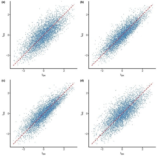
1. Introduction
Empirical applications of unit root testing procedures commonly face uncertainty as to which test to use when there is a large battery of methods to choose from but no a priori information in favour of one procedure is available. Often, there are unknown characteristics of the data generating process (DGP) that favour some testing procedure(s). Examples include uncertainty about the initial condition or about deterministic patterns. Both imply the risk of low power when applying an inferior testing procedure; see Müller and Elliott (2003) and Elliott et al. (1996). It then is common practice to apply the whole set of tests and to jointly interpret the results. Such an approach is, however, problematic when not all/some tests reject the null, i.e., when there are “mixed signals”. This is a non-negligible issue in (panel) cointegration testing, in particular when the tests under consideration are from distinct classes (Gregory et al. 2004; Hanck 2012). This problem also occurs in empirical studies that employ multiple panel unit roots tests (PURTs). For example, Hurlin (2010) studied stochastic trends in fourteen macro and financial variables from the seminal paper by Nelson and Plosser (1982) using OECD panel data and partly obtains ambiguous results. Mullineux et al. (2010) analysed financial integration in EU economies using flows of funds data and found mixed results for the convergence of equity and internal financing using a battery of PURTs.
Two nonstationary volatility robust PURTs proposed by Demetrescu and Hanck (2012a) and Herwartz and Siedenburg (2008), and henceforth, may confront the researcher with a similar situation. Simulation evidence shows that has better size-control than and that power of the tests is different under various forms of cross-sectional dependence and heteroskedasticity. The extent of these differences depends on the degree and type of both cross-sectional dependence and variance breaks—characteristics which are generally unknown in applications. Moreover, although both statistics are nonstationary volatility robust versions of the test in Breitung and Das (2005), different size and power characteristics suggest that mixed signals may occur.1 This might be especially problematic under the alternative when the tests are applied in small to medium-sized panels because the power differential may then be large.
As mixed signals imply imperfect correlation among and , a strategy to “reject at level if the most significant test outcome implies rejection” is invalid since the actual size of the strategy will generally be larger than . These considerations demand a joint test decision by means of a multiple testing procedure which controls size.
The aim of this paper is to analyse the prevalence of mixed signals from and and to suggest a simple but effective multiple testing method (cf. Simes 1986) which tackles the issues outlined above. The test is a modification of the Bonferroni correction and has been shown to be more powerful when the underlying test statistics are positively dependent under the null; see Sarkar (1998). An empirical application investigates the trend behaviour of inflation rates of OECD countries by means of the individual and the combined test. We thus reinvestigate some of the results presented in Culver and Papell (1997) by using the original dataset from February 1957 to September 1994 as well as for a longer observation period which also covers the recent three decades. Cross-dependence and heteroskedasticity are marked features of the data, stressing the need to apply robust PURTs.
Section 2 introduces the econometric framework and briefly discusses both test statistics. Section 3 provides Monte Carlo results which investigate the prevalence of mixed signals among and . We then present the multiple testing strategy and compare the performance of both tests with the combined test. Section 4 discusses the application to inflation rates. Section 5 concludes.
2. Econometric Framework and Robust PURTs
2.1. Panel Model and Assumptions
We consider a first-order autoregressive panel model with time-varying second moments,
where , and the errors are and . The PURTs (cf. Section 2.2) are designed for testing the unit root null hypothesis against the homogenous alternative using a test statistic from a pooled regression.
Following Herwartz et al. (2016), we impose the following assumptions on which basically mirror the framework used in Breitung and Das (2005) but allow for the time-dependent variability of in addition to weak cross-sectional dependence.
Assumption
- (i)
- The are serially uncorrelated with and variance-covariance matrices for all t.
- (ii)
- The are positive definite with positively bounded eigenvalues for all t.
- (iii)
- for all where the u are elements of .
Assumption implies that the innovations are uncorrelated over time. Assumption allows for weak forms of cross-dependence between the series in Equation (1). Regarding heteroskedasticity, covers both discrete shifts and patterns of trending (co)variances which are consistent with the assumption that has bounded eigenvalues.2 Assumption is a common assumption in the panel literature and demands finite fourth moments of the (and thus the ).
2.2. Volatility-Break Robust Panel Unit Root Tests
This section briefly reviews the two PURTs under study here.
2.2.1. The White-Type Test with Cauchy Instrumenting
The robust homogenous PURT proposed by Demetrescu and Hanck (2012a) builds on the work of So and Shin (1999), who found that the “Cauchy” estimator of the autoregressive coefficient in a univariate AR(1) model has a Gaussian limit even under the unit root null. The statistic
is an adaption to dependent panels that has been proposed by Shin and Kang (2006). They account for cross-dependence by using orthogonalised residuals ; denotes recursively mean-adjusted lagged levels.3 Demetrescu and Hanck (2012b) show that retains its asymptotic properties under unconditional heteroskedasticity thanks the transformation of the information in the individual series by the sign function . A shortcoming of is the orthogonalisation procedure, as it requires for reasonable size (Demetrescu and Hanck 2012b). To circumvent this, Demetrescu and Hanck (2012a) suggest a modification of the Shin and Kang (2006) test which involves a White (1980) covariance estimator. The test statistic is computed as
where . Motivated by the Gaussian limiting null distribution of and Monte Carlo evidence, is used with standard normal critical values. The test is reported to perform well under factor-type cross-dependence as well as nonstationary volatility.
2.2.2. The White-Type Test
Herwartz and Siedenburg (2008) proposed the test statistic
related to in also using a panel generalisation of the heteroskedasticity-consistent White (1980) covariance estimator.
Herwartz and Siedenburg (2008) conjecture that the White correction renders robust to general forms of heteroskedasticity. Herwartz et al. (2016) indeed proved that is asymptotically Gaussian under variance shifts. They suggest that, hence, using Cauchy instruments in Equation (3) is not necessary for asymptotic standard normality. This, however, does not render superfluous as it turns out that the tests have distinct characteristics both under the null and the alternative: Simulation evidence in Section 3.3.1 confirms that has more reliable size control and that the power of the tests is different in small to medium-sized panels under cross-dependence and various scenarios of breaks in the innovation variance.
2.2.3. Data Preprocessing
In order for and to be valid in applications where Equation (1) is unlikely to hold given (possibly distinct) patterns of short-run dynamics in the series, it is necessary to prewhiten the data. This can be done as proposed in Breitung and Das (2005).
where the are ordinary least squares (OLS) estimates from individual regressions . The are chosen using a consistent order selection criterion.
Similarly, the test statistics are not pivotal if the data exhibit deterministic patterns such as nonzero intercepts or linear time trends under the alternative. While it is nontrivial to account for the latter, individual specific intercepts may be efficiently removed by recursive demeaning (So and Shin 2001, see footnote 3) or by subtracting the first observations from the level series (Breitung and Das 2005).4 Since Herwartz et al. (2016) reported and to be slightly less powerful when the data are recursively demeaned, we use the latter approach and prewhiten the data beforehand as in Equation (5), if necessary.
3. Mixed Signals and a Combined Testing Procedure
This section examines the prevalence of mixed signals when and are applied to the same data for various scenarios of cross-sectional dependence and variance, described in Section 3.1. Section 3.2 discusses the results. We then propose our alternative testing procedure based on the multiple test by Simes (1986) and compare its performance with that of and in Section 3.3.
3.1. Simulation Setup
The setup follows the design in Herwartz et al. (2016), which considers the following DGPs:
where bold symbols are , is a vector of ones, and ⊙ denotes elementwise products. DGP A generates panels with uncorrelated errors. DGP B allows to investigate the performance under serial correlation for with denoting the uniform distribution on . Under the null, so that both DGPs generate driftless panel random walks. Under , with , yielding processes with heterogenous degrees of persistence and individual effects .
Under cross-sectional independence, we set . We further consider the three following scenarios for simulating cross-sectional dependence.
- Spatial Correlation: Contemporaneous correlation is introduced by a first-order spatial autoregressive (SAR) process in the following innovations:where the scalar spatial AR coefficient governs strength of the dependence. is a symmetric row-normalised spatial weights matrix of the one-ahead-and-one-behind type. Elements of one ahead and one behind the main diagonal are set to and zeros elsewhere; see Baltagi et al. (2007).5 is set to throughout.
Both a one-factor structure and equicorrelation imply strong cross-sectional dependence in the terminology of Breitung and Pesaran (2008) and thus violate assumption .6 They hence serve to study the robustness properties of the tests considered here.
To incorporate unconditional heteroskedasticity, we introduce variance breaks. Breaks can occur at time so that
where , , and is the indicator function. The setup allows for k different variance regimes, where for convenience such that can be interpreted as the scaling factor for the jth regime’s standard deviation relative to the first regime. We consider break scenarios from Cavaliere and Taylor (2007) who found that in cases with two variance regimes, size and power of common time series unit roots tests deteriorate considerably when there are early negative (, ) or late positive (, ) volatility shifts. Thus, it is interesting to investigate the performance of a combined test under these circumstances.
We consider all combinations of and and use a burn-in period of 50 observations in order to avoid dependence on initial conditions under the alternative. If not stated otherwise, we use 25,000 replications and test at the 5% level using the corresponding Gaussian critical value. Size-adjusted critical values are used for power comparisons.
3.2. Evidence of Mixed Signals
As shown in Herwartz et al. (2016), and have distinct performances when applied in small to medium-sized samples. While has better size control, is often but not uniformly more powerful. The extent of these differences depends on both the type of cross-sectional dependence, time or degree of a structural break in the unconditional variance, and serial dependence. As these characteristics of the data are generally unknown, it is nontrivial to draw conclusions when one test rejects the null while the other does not—a so-called “mixed signal”.
Clearly, the relevance of this issue is linked to its likelihood of occurrence. Therefore, we conduct a simulation study along the lines of Gregory et al. (2004).7 We first use the simulated tests statistics to compute empirical p-values by taking rank order across the empirical distribution and dividing by M. For these pairs of empirical significance levels, empirical correlations are computed in order to gauge the degree of similarity in test outcomes under the null. Then, we investigate rejections both under the null and the alternative when the tests are applied to the same data. More specifically, we compute the proportions of joint rejection using size-adjusted critical values. At last, and probably most interestingly, the proportion of cases where one test rejects and the other one retains the null is assessed. This is our measure for the likelihood of obtaining ambiguous test outcomes.
3.2.1. Results
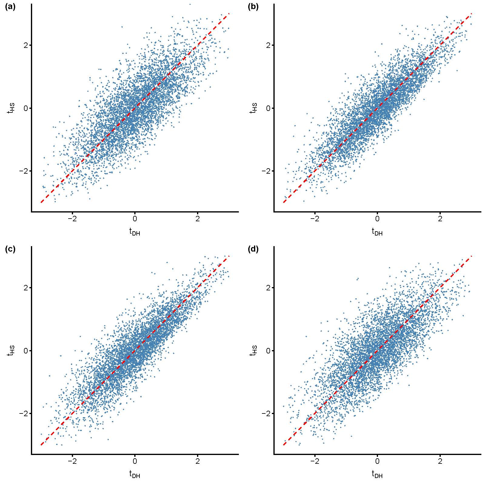
Figure 1 gives indications for mixed signals under the null. It displays probits of empirical p-values obtained for four scenarios of cross-dependence under an early variance break. While the plots demonstrate positive correlation for and , we find evidence for ambiguous test decisions in all four scenarios of cross-dependence. Table 1 presents empirical correlations of p-values and proportions of joint rejections and mixed signals under the null and under the alternative.
Under the null, we confirm moderate to high correlations of empirical p-values. Furthermore, rates of joint rejections (mostly ranging below 3%) are uniformly smaller than rates of mixed outcomes, i.e., the tests are likely to produce contradictory outcomes. These results show little variation across N and T for all scenarios of cross-dependence and variance regimes. This suggests that the findings are relevant for datasets that are commonly used in empirical application and that the issue does not alleviate quickly with larger panels.
A somewhat different picture emerges under the alternative where joint rejection rates naturally improve in N and T due to consistency of both tests. However, proportions of mixed outcomes differ: They are linked to the difference in power between and , which it turn depends on N and T as well as the time and the degree of variance breaks; see Herwartz et al. (2016).8 Our results indicate that mixed signals occur in all scenarios of cross-dependence and heteroskedasticity where the pattern is often similar: The probability of observing contradicting results is low to moderate when T is small relative to N, increases for panels of moderate dimensions, and then decreases towards zero as N and T get large. The proportion of mixed signals may be higher than 20%. An explanation is that one of the tests is often more powerful than the other such that the dissimilarity between test outcomes may be high. This is in contrast to larger panels where the additional amount of information against the null drives both tests towards rejection, viz. coinciding results are more likely. Furthermore, Table 1 indicates that mixed signals under the alternative cannot always be attributed to the less powerful test not rejecting. This is observed in all scenarios of cross-dependence under a late positive variance shift.
In summary, the results show that, despite the similar design of and , a researcher is likely to encounter mixed signals when both tests are applied to the same data.
3.3. A Combined Testing Procedure
Consider the p-values obtained from suitably testing the individual null hypotheses such that under . The so-called Bonferroni correction for testing the global or intersection null hypothesis rejects when
Equation (12) allows to test the global null, controlling the family-wise error rate at . A particular merit of Equation (12) is that it does not require assumptions about the joint distribution of the underlying test statistics or their dependence. However, the procedure may be quite conservative and may have low power.
As an alternative, we consider the following modified Bonferroni procedure proposed by Simes (1986).
Simes’ Test
- Obtain ordered p-values of n tests
- Reject the global null if
Consider the case . Simes’ test rejects at if or .
Simes (1986) proves that Equation (13) yields a conservative test provided the test statistics are independent. Simulation evidence in Simes (1986) also suggests that Equation (13) dominates the classical Bonferroni procedure if the individual tests statistics are highly positively correlated. Sarkar (1998) established conservativeness of Equation (13) for test statistics of which the joint null distribution is “multivariate totally positive of order 2” (), a substantially weaker assumption than that of independence which covers a rather large family of multivariate distributions.
Given the various positive correlations of and in the scenarios of cross-dependence and variance breaks, the simplicity and robustness to (certain forms of) positive dependence render Equation (13), henceforth S, a promising candidate for a combined test.9 It is unclear whether the joint distribution of the tests is , and we do not give a proof. It has, however, been shown that the condition can be relaxed even further; see Sarkar (2008). To what extent S is of use in our setting is discussed by means of the simulation results discussed next.
3.3.1. Results
Table A1, Table A2, Table A3 and Table A4 report empirical rejection frequencies. The left panels correspond to DGP A while the right panels refer to DGP B. We confirm the finite sample results for and presented in Herwartz et al. (2016), i.e., distinct small-sample properties both under the null and under the alternative. Performance is also mostly satisfying under serial correlation. However, then is somewhat conservative for small T. Both tests have lower power than under uncorrelated disturbances. The results do not deteriorate much when weak-form cross-dependence imposed by Assumption is violated as is the case under equicorrelation and the common factor structure.
Turning to the S test, we find it does well in combining information from and . Under the null, S is often closer to the nominal level of 5% than and does compete well with the empirical size of . Under independence and spatial correlation, the size of S is best when N and T are large and when T is large relative to N. This is also the case under serially correlated disturbances, a setting that highlights a slight downside of S’s property to track the performance of under the null: S is undersized when produces too few rejections. While this behaviour is not overly pronounced, it stresses the need for larger samples when adjusting the data for short-run dynamics in applications. Largely, the same conclusions are obtained for equicorrelated panels and under a common factor, except that S is slightly conservative.
In terms of power, S typically tracks the more powerful of the individual tests. Nonetheless, S seems superior to simultaneously applying both tests, let alone application of only one test. S is especially beneficial in small to medium-sized panels where is often more powerful than as mixed signals are more likely; see Section 3.2 and Table 1.
We conclude that combining information from and may be beneficial for the following reasons: First, S avoids the choice either to risk size-distortions or low power in applications of only one test. Second, S circumvents the risk of mixed signals when using both tests. Both scenarios have been confirmed to be relevant in our simulation studies. Third, application of S is attractive in terms of simplicity because it comes with virtually no additional expense in computation. This is in contrast to other prominent methods used in meta-analysis such as, e.g., the p-value combination tests in Fisher (1932) and Stouffer et al. (1949) and modifications thereof as in Hartung (1999) and more recent contributions to the unit root literature like the union of rejections tests in Harvey et al. (2009). All these depend on the particular correlation structure of the test statistics and therefore require, e.g., use of resampling techniques.
4. Application to Inflation Rates
Since, at least, Nelson and Plosser (1982), it has been argued that inflation may follow a stochastic trend. The persistence of inflation has far-reaching implications for the analysis and interpretation of fundamental economic relationships. This includes structural models of, e.g., different Phillips curve concepts and numerous models that rely upon price rigidities or the trending behaviour of the real interest rate, a major determinant of savings and investment (Culver and Papell 1997; Rose 1988). Further, the behaviour of inflation is important for central banks’ monetary policy rules.
Empirical research arrives at different conclusions. There is pioneering work reporting stationarity, for example, Rose (1988), who investigated the stability of the U.S. real interest rate, and Barsky (1987), who analysed U.S. inflation and reported stationarity for subperiods. On the other hand, some authors found evidence that inflation is I(1), e.g., Johansen (1992), Ball and Cecchetti (1990), and Johansen and Juselius (2001).
More recent contributions reinvestigate the issue, e.g., Culver and Papell (1997), who studied monthly panel data for thirteen OECD countries ranging from February 1957 to September 1994. They found evidence for nonstationarity using ADF and KPSS tests but acknowledged the shortcomings of these tests and thus resorted to PURTs.10 Their panel approach is based on the test by Levin et al. (2002) and rejects the unit root null even for various 4-element subsets of countries. A follow-up contribution by Basher and Westerlund (2008) revisits these conclusions as the employed testing procedure is not robust to cross-dependence and heteroskedasticity. Hence, one should be cautious in attributing different outcomes of time series and panel approaches to potential power gains from exploiting the additional variation in the cross-section dimension. As noted by Basher and Westerlund (2008), this is problematic as structural changes such as variance breaks tend to be more likely in macro series when long data spans are considered and comovements are strong. Basher and Westerlund (2008) reported results from second-generation PURTs which suggest that stationarity of inflation holds after accounting for general forms of cross-sectional dependence and structural breaks.
Next, we reconsider some of the conclusions in Culver and Papell (1997) by applying , , and S to several panels of OECD inflation rates.11 We consider two datasets and a total of four observation periods. First, the original monthly consumer price index (CPI) data from Culver and Papell (1997) from February 1957 to September 1994. Second, we use a larger set of monthly CPI data from April 1961 to March 2019 obtained from the OECD database for which we also consider two subperiods of roughly 30 years for robustness checks. These range from April 1961 to December 1989 and from January 1990 to March 2019. It is interesting to study evidence for these subsamples as they reflect different patterns of macroeconomic activities that led to structural shifts in volatility. This is particularly the case for the significantly less volatile last three decades which are marked by the advent of inflation targeting.
4.1. Preliminary Analysis
Figure 2 plots year-on-year inflation rates of all countries for the longest observation span. Two characteristics shared by most of the series which are crucial for conducting inference based on PURTs are rather obvious: Eyeballing shows considerable comovement suggesting cross-dependence to be accounted for. Additionally, the moderate period up to the mid-1970s lapses into a highly volatile period which is then followed by a marked downward shift in volatility at the beginning of the 1990s. Reduced volatility persists for the following decades up to a kink situated around the financial crisis in 2008. These findings are supported by means of Figure 3 displaying quartiles for the sample distribution of inflation rates across the economies. The distribution’s spread corresponds to previously identified regimes, i.e., moderate variance at the beginning of the sample, followed by a quickly extending interquartile range which diminishes again beyond 1990 and emerges into a more stable period characterised by low volatility. The findings thus suggest three distinct variance regimes.
We may further assess second moment variability via estimated variance profiles, i.e.,
as proposed by Cavaliere and Taylor (2007).12 Figure 4 shows that, for all four subsamples, none of the estimated variance profiles are close to the dashed red line, the theoretical profile of a homoskedastic series. The profiles display patterns suggesting that the volatility of most series experienced a positive break followed by a downward trend. Consider, e.g., Spanish inflation, which shows a sharp upward shift after about 20% and 30% of the sample that is followed by a moderation. Further, the profiles of some economies show very similar patterns, for instance, those of Italy and the United Kingdom. In this regard, the profiles for the recent three decades are particularly interesting as they display a global decrease in volatility and a considerable degree of convergence at the beginning of the recent financial crisis. This tendency of synchronous variance regime switching may also be seen as an indicator for economic comovement.
Culver and Papell (1997) used a simple dynamic panel approach allowing for country-specific fixed effects. The autoregressive coefficients are restricted to be equal for all cross sections. Thus, inflation is modelled by a panel autoregressive process
Since it is plausible that the data exhibits short-run dynamics as well as nonzero fixed effects, the individual tests are conducted on prewhitened data that are subsequently centered by means of first observations as we expect inflation rates to have nonzero means under stationarity. The Schwarz information criterion (SIC) is used to determine the maximum optimal lag order which is then used for the prewhitening procedure of Section 2.2.3.
4.2. Results from Robust PURTs
Table 2 presents the results of the analysis for eleven groups of countries. We first compare results for the data from Culver and Papell (1997). We find that , , and S coincide and strongly reject the null of a panel unit root at the 1% level, except for the group of G7 countries where S rejects only at 5%. Virtually the same results are obtained for year-on-year inflation rates from April 1961 to March 2019 where all tests find strong evidence against the null with the exception of S, which rejects only at 5% for the group of non-G7 economies.
For the subsample from April 1961 to Dec. 1989, we find weaker evidence against the null as S rejects mostly at 5%. A distinctive feature here is that and produce mixed signals at 5% for all groupings except the G7 and the “unit root seven” where S retains the null at 10%.
Turning to the less volatile period from January 1990 to March 2019, mixed signals are found for all groups since does not reject once but finds evidence at 10%, except for group k. However, combining significance by S does not reject the null even at 10% as p-values for do not fall below the lower cutoff of 0.05 for any of the groupings. This is a rather peculiar finding as nonstationarity of inflation rates implies no mean reversion which we presume to be an effect of inflation targeting, alongside reduced volatility. A possible explanation is that structural change due to increased integration of monetary policy implies the downward shift in volatility and stronger cross-dependence. Both are observed characteristics of the subsample which were shown to result in lower power of the tests.
Culver and Papell (1997) further assess how much cross-section variation is required for rejection of the unit root null by computing all possible combinations of countries in panels of sizes . They report that, strikingly, any combination of five countries is already sufficient for rejection at 5% in all panels. We reinvestigate this issue for both datasets using S and also report rejection rates for and to gauge for the potential of observing mixed evidence. Table 3 presents the results.
As expected, our results for the original data are somewhat weaker but confirm that the null is rarely accepted in panels of five economies. Evidence against the null increases markedly as we turn to combinations of six and more countries. S rejects nonstationarity at 1% in almost 80% of all combinations of seven economies. We find similar results for the extended observation period of year-on-year inflation rates where S rejects at 1% in 87.1% of all possible combinations for . The results for April 1961 to Dec. 1989 also show considerable evidence against the null for , although the proportion of strong rejections is noticeably lower and most rejections occur at 5%. Finally, the results presented in the bottom panel underline that the recent three decades provide conspicuously little evidence in favour of the alternative since the proportion of combinations in which the null is not rejected ranges above 75%, even in panels of five or more economies. Another result is that the tendency for mixed signals is high, especially when testing at 5% based on year-on-year rates from April 1961 to Dec. 1989. For this subsample, retains the null far more often than , such that it appears worthwhile to rely on the combined evidence of S.
Altogether, evidence from the S test suggests robustness of the finding of stationarity of inflation in Culver and Papell (1997) when we account for variance breaks and weak cross-dependence for both the original dataset and the extended sample of year-on-year inflation rates. The results for the recent three decades point towards nonstationarity, which contradicts the notion that inflation targeting establishes a stable regime of low inflation rates. This finding should be considered with caution as it might be due to structural breaks in the intercept which may not be well-handled by the tests.
5. Conclusions
This article investigates the performance of two recently proposed homogenous panel unit root tests, the White-type tests proposed by Herwartz and Siedenburg (2008) and its Cauchy counterpart suggested by Demetrescu and Hanck (2012a). Both are tailored for applications to weakly cross-dependent data that exhibit nonstationary volatility such as breaks in the unconditional variance. Our Monte Carlo studies confirm that the Cauchy counterpart has better size-control but is less powerful than the White-type test when applied in small to medium-sized samples. A common practice in such a situation is to apply both tests and to interpret the results jointly. This is shown to be problematic: We find that the tests are imperfectly correlated under the null and have a tendency to produce contradicting test outcomes which are not straightforward to interpret. The extent of this issue is found to depend on the type and degree of the cross-sectional dependence in the data. Prevalence of mixed signals is shown to be most pronounced under the alternative in small to medium-sized samples when the power differential of the tests is large. This is problematic for the applied researcher, as it is inadmissible to simply follow the decision of the rejecting test or some related rejection rule which ignores the multiple testing nature of the problem. As a remedy, we suggest combining information from both tests using the improved Benferroni procedure proposed by Simes (1986). Simulation evidence reveals that this simple approach does well in controlling size and has power close to the more powerful individual test.
An empirical application reinvestigates whether there is a unit root in year-on-year inflation rates using panels of monthly data for selected OECD countries. Our findings are twofold. We establish robustness of the results by Culver and Papell (1997), who reported stationarity for monthly inflation rates. The combined test also rejects the null for year-on-year inflation rates observed over an extended sample span which also covers the recent three decades. On the other hand, we find little evidence for stationarity when applying the combined test to a subsample of the last thirty years—a result which may be attributed to ongoing structural change and thus should be treated with caution as the tests may lack power under such conditions. This issue could be investigated using PURTs that allow for breaks both in the variance and in the mean which is, however, beyond the scope of this paper.
Future research could extend the multiple testing procedure towards models that include a linear trend under the alternative. It could also be worthwhile to investigate the benefits of applying the procedure to other PURTs as it is not restricted to the volatility-break robust tests considered here. Furthermore, it would be interesting to systematically compare the performance of Simes’ test with other meta tests that are less reliable if the information to be combined is not independent. A feasible path to be followed is resampling, e.g., using the wild bootstrap procedure suggested by Herwartz and Walle (2018).
Author Contributions
Conceptualization, M.C.A. and C.H.; methodology, M.C.A. and C.H.; software, M.C.A.; validation, M.C.A.; formal analysis, M.C.A. and C.H.; investigation, M.C.A.; resources, M.C.A. and C.H.; data curation, M.C.A.; writing—original draft preparation, M.C.A. and C.H.; writing—review and editing, M.C.A. and C.H.; visualization, M.C.A.; supervision, C.H.; project administration, M.C.A. and C.H.; funding acquisition, C.H.
Funding
The authors gratefully acknowledge financial support of the German Research Foundation (DFG) through the Collaborative Research Center 823 “Statistical Modelling of Nonlinear Dynamic Processes”, project A4.
Conflicts of Interest
The authors declare no conflict of interest.
Abbreviations
The following abbreviations are used in this manuscript:
| ADF | augmented Dickey-Fuller |
| CPI | consumer price index |
| DGP | data generating process |
| I(1) | integrated of order one |
| EU | European Union |
| KPSS | Kwiatkowski–Phillips–Schmidt–Shin |
| multivariate totally positive of order 2 | |
| OECD | Organisation for Economic Co-operation and Development |
| PURT | panel unit root test |
| SIC | Schwarz information criterion |
Appendix A

Table A1.
Rejection frequencies in cross-sectionally independent panels. , . DGP B: . Power is computed using size-adjusted 5% critical values; 25,000 replications were used.
Table A1.
Rejection frequencies in cross-sectionally independent panels. , . DGP B: . Power is computed using size-adjusted 5% critical values; 25,000 replications were used.
| DGP A | DGP B | ||||||||||||||||||
|---|---|---|---|---|---|---|---|---|---|---|---|---|---|---|---|---|---|---|---|
| Size | Power | Size | Power | ||||||||||||||||
| Homoskedasticity | |||||||||||||||||||
| 10 | 25 | 5.1 | 6.4 | 4.9 | 18.9 | 25.2 | 23.1 | 3.5 | 6.2 | 4.0 | 15.0 | 18.0 | 17.6 | ||||||
| 10 | 50 | 5.4 | 6.6 | 5.2 | 39.8 | 54.4 | 51.5 | 4.0 | 6.4 | 4.4 | 35.4 | 47.0 | 45.0 | ||||||
| 10 | 100 | 5.2 | 7.0 | 5.3 | 76.7 | 85.6 | 86.6 | 4.4 | 6.6 | 4.6 | 72.1 | 82.3 | 83.2 | ||||||
| 10 | 250 | 5.2 | 7.2 | 5.6 | 98.8 | 98.2 | 99.5 | 4.5 | 6.6 | 4.7 | 98.7 | 98.2 | 99.5 | ||||||
| 50 | 25 | 5.2 | 5.5 | 4.5 | 59.0 | 77.0 | 73.8 | 3.1 | 8.8 | 4.9 | 44.5 | 55.5 | 55.5 | ||||||
| 50 | 50 | 4.9 | 5.8 | 4.8 | 96.5 | 99.1 | 99.1 | 3.7 | 7.0 | 4.5 | 91.8 | 97.4 | 97.5 | ||||||
| 50 | 100 | 4.9 | 5.5 | 4.6 | 100.0 | 100.0 | 100.0 | 4.3 | 6.3 | 4.6 | 100.0 | 100.0 | 100.0 | ||||||
| 50 | 250 | 5.0 | 6.0 | 4.9 | 100.0 | 100.0 | 100.0 | 4.3 | 5.6 | 4.3 | 100.0 | 100.0 | 100.0 | ||||||
| Early negative shift | |||||||||||||||||||
| 10 | 25 | 5.0 | 6.0 | 4.3 | 7.7 | 8.9 | 8.7 | 3.7 | 6.7 | 4.1 | 5.9 | 6.0 | 6.0 | ||||||
| 10 | 50 | 4.8 | 6.4 | 4.8 | 15.7 | 20.2 | 18.8 | 3.1 | 6.3 | 3.8 | 13.2 | 15.4 | 14.8 | ||||||
| 10 | 100 | 5.1 | 6.5 | 4.9 | 36.0 | 50.8 | 48.2 | 3.6 | 6.4 | 4.1 | 32.3 | 43.6 | 42.6 | ||||||
| 10 | 250 | 5.1 | 6.9 | 5.3 | 79.0 | 91.7 | 91.4 | 4.1 | 6.5 | 4.7 | 76.2 | 89.8 | 89.6 | ||||||
| 50 | 25 | 5.1 | 5.3 | 4.3 | 13.8 | 18.0 | 16.7 | 3.9 | 10.5 | 6.1 | 6.2 | 3.7 | 4.4 | ||||||
| 50 | 50 | 5.0 | 5.4 | 4.4 | 46.9 | 64.8 | 61.2 | 2.6 | 9.1 | 5.0 | 35.0 | 34.5 | 35.9 | ||||||
| 50 | 100 | 5.0 | 5.5 | 4.5 | 93.2 | 98.9 | 98.7 | 3.0 | 7.4 | 4.5 | 89.2 | 95.8 | 96.7 | ||||||
| 50 | 250 | 4.9 | 5.8 | 4.7 | 100.0 | 100.0 | 100.0 | 3.9 | 6.5 | 4.6 | 100.0 | 100.0 | 100.0 | ||||||
| Late positive shift | |||||||||||||||||||
| 10 | 25 | 5.2 | 5.4 | 4.0 | 15.7 | 17.3 | 17.0 | 4.1 | 4.8 | 3.4 | 11.3 | 13.1 | 12.5 | ||||||
| 10 | 50 | 5.1 | 5.8 | 4.5 | 32.9 | 35.9 | 34.8 | 4.3 | 5.8 | 4.0 | 26.5 | 27.8 | 29.3 | ||||||
| 10 | 100 | 4.9 | 6.3 | 4.7 | 69.6 | 66.9 | 71.8 | 4.9 | 6.5 | 4.9 | 59.1 | 58.8 | 62.8 | ||||||
| 10 | 250 | 4.8 | 6.6 | 5.0 | 98.7 | 94.2 | 98.5 | 4.9 | 6.4 | 4.9 | 97.7 | 92.9 | 97.7 | ||||||
| 50 | 25 | 4.8 | 4.9 | 3.7 | 46.2 | 49.4 | 50.0 | 4.0 | 6.6 | 3.8 | 27.9 | 29.9 | 31.7 | ||||||
| 50 | 50 | 5.2 | 5.6 | 4.4 | 88.4 | 87.1 | 90.1 | 5.2 | 7.8 | 5.2 | 72.8 | 75.3 | 78.8 | ||||||
| 50 | 100 | 5.1 | 5.6 | 4.6 | 100.0 | 99.6 | 100.0 | 5.1 | 6.9 | 5.1 | 99.6 | 99.2 | 99.8 | ||||||
| 50 | 250 | 5.3 | 5.9 | 5.1 | 100.0 | 100.0 | 100.0 | 5.5 | 6.8 | 5.2 | 100.0 | 100.0 | 100.0 | ||||||
Table A2.
Rejection frequencies in cross-dependent panels—spatial correlation. , , . DGP B: . Power is computed using size-adjusted 5% critical values; 25,000 replications were used.
Table A2.
Rejection frequencies in cross-dependent panels—spatial correlation. , , . DGP B: . Power is computed using size-adjusted 5% critical values; 25,000 replications were used.
| DGP A | DGP B | ||||||||||||||||||
|---|---|---|---|---|---|---|---|---|---|---|---|---|---|---|---|---|---|---|---|
| Size | Power | Size | Power | ||||||||||||||||
| Homoskedasticity | |||||||||||||||||||
| 10 | 25 | 5.5 | 7.3 | 5.1 | 11.1 | 12.0 | 11.7 | 3.3 | 5.4 | 3.1 | 10.6 | 11.2 | 11.5 | ||||||
| 10 | 50 | 5.8 | 7.8 | 5.6 | 20.8 | 23.8 | 23.2 | 4.3 | 6.6 | 4.3 | 19.2 | 22.0 | 21.4 | ||||||
| 10 | 100 | 5.8 | 8.1 | 5.9 | 43.2 | 48.2 | 47.4 | 5.2 | 7.7 | 5.4 | 39.2 | 44.2 | 43.4 | ||||||
| 10 | 250 | 5.9 | 8.4 | 6.0 | 80.6 | 83.6 | 84.8 | 5.3 | 8.0 | 5.5 | 78.5 | 81.7 | 82.6 | ||||||
| 50 | 25 | 5.4 | 6.1 | 4.6 | 30.3 | 36.3 | 34.8 | 3.2 | 6.3 | 3.6 | 24.1 | 26.6 | 26.7 | ||||||
| 50 | 50 | 5.4 | 6.4 | 5.0 | 67.3 | 74.4 | 73.5 | 3.9 | 6.3 | 4.2 | 60.2 | 67.1 | 66.4 | ||||||
| 50 | 100 | 5.3 | 6.5 | 5.0 | 96.8 | 97.8 | 98.2 | 4.5 | 6.7 | 4.6 | 94.9 | 96.4 | 96.9 | ||||||
| 50 | 250 | 5.5 | 6.9 | 5.2 | 100 | 100 | 100 | 4.8 | 6.5 | 4.9 | 100 | 100 | 100 | ||||||
| Early negative shift | |||||||||||||||||||
| 10 | 25 | 5.1 | 6.3 | 4.5 | 6.0 | 5.9 | 5.9 | 3.4 | 5.4 | 3.2 | 5.0 | 4.7 | 4.9 | ||||||
| 10 | 50 | 5.6 | 7.1 | 5.0 | 8.6 | 9.6 | 9.4 | 3.3 | 5.4 | 3.1 | 8.6 | 9.2 | 9.2 | ||||||
| 10 | 100 | 5.5 | 7.7 | 5.5 | 18.8 | 21.1 | 20.5 | 4.0 | 6.6 | 4.2 | 17.7 | 19.5 | 19.3 | ||||||
| 10 | 250 | 5.5 | 7.9 | 5.6 | 47.3 | 53.5 | 52.4 | 4.6 | 7.5 | 5.0 | 44.9 | 50.3 | 50.0 | ||||||
| 50 | 25 | 5.1 | 5.9 | 4.4 | 8.8 | 9.3 | 9.3 | 3.4 | 7.1 | 4.1 | 5.7 | 4.5 | 4.8 | ||||||
| 50 | 50 | 5.2 | 6.4 | 4.8 | 23.8 | 28.0 | 26.8 | 2.8 | 6.6 | 3.6 | 20.0 | 19.3 | 19.5 | ||||||
| 50 | 100 | 5.3 | 6.5 | 5.0 | 61.5 | 72.2 | 69.5 | 3.3 | 6.2 | 3.8 | 57.0 | 65.0 | 64.4 | ||||||
| 50 | 250 | 5.3 | 6.5 | 4.9 | 97.4 | 99.5 | 99.3 | 4.2 | 6.5 | 4.5 | 96.3 | 99.2 | 99.1 | ||||||
| Late positive shift | |||||||||||||||||||
| 10 | 25 | 5.3 | 6.1 | 4.4 | 10.5 | 10.3 | 10.5 | 3.4 | 4.0 | 2.6 | 8.3 | 9.0 | 8.8 | ||||||
| 10 | 50 | 5.4 | 6.6 | 4.9 | 18.8 | 18.4 | 18.8 | 4.5 | 5.4 | 3.8 | 14.6 | 15.8 | 15.7 | ||||||
| 10 | 100 | 5.5 | 7.3 | 5.2 | 37.3 | 34.1 | 37.4 | 4.9 | 6.4 | 4.5 | 32.5 | 31.3 | 33.3 | ||||||
| 10 | 250 | 5.7 | 8.1 | 5.8 | 78.0 | 67.5 | 76.2 | 5.6 | 7.7 | 5.4 | 72.6 | 64.0 | 71.5 | ||||||
| 50 | 25 | 5.0 | 5.6 | 4.2 | 24.8 | 22.6 | 24.6 | 3.7 | 4.9 | 3.0 | 16.9 | 17.4 | 17.8 | ||||||
| 50 | 50 | 5.1 | 6.0 | 4.4 | 56.7 | 49.1 | 55.9 | 4.6 | 6.2 | 4.3 | 43.0 | 39.6 | 43.1 | ||||||
| 50 | 100 | 5.4 | 6.4 | 5.0 | 92.0 | 82.9 | 90.6 | 5.2 | 6.6 | 4.9 | 86.1 | 77.8 | 84.8 | ||||||
| 50 | 250 | 5.5 | 6.8 | 5.1 | 100 | 99.6 | 100 | 5.4 | 6.6 | 5.0 | 100 | 99.5 | 100 | ||||||
Table A3.
Rejection frequencies in cross-dependent panels—equicorrelation. , , . DGP B: . Power is computed using size-adjusted 5% critical values; 25,000 replications were used.
Table A3.
Rejection frequencies in cross-dependent panels—equicorrelation. , , . DGP B: . Power is computed using size-adjusted 5% critical values; 25,000 replications were used.
| DGP A | DGP B | ||||||||||||||||||
|---|---|---|---|---|---|---|---|---|---|---|---|---|---|---|---|---|---|---|---|
| Size | Power | Size | Power | ||||||||||||||||
| Homoskedasticity | |||||||||||||||||||
| 10 | 25 | 5.4 | 6.6 | 4.9 | 13.6 | 15.9 | 15.1 | 3.3 | 5.1 | 3.0 | 11.6 | 13.3 | 13.2 | ||||||
| 10 | 50 | 5.7 | 7.4 | 5.3 | 25.2 | 30.4 | 28.9 | 4.4 | 6.4 | 4.3 | 23.1 | 27.1 | 26.4 | ||||||
| 10 | 100 | 5.8 | 7.7 | 5.8 | 48.9 | 54.0 | 53.2 | 4.8 | 7.3 | 5.0 | 46.1 | 50.6 | 50.3 | ||||||
| 10 | 250 | 5.9 | 7.8 | 5.8 | 81.8 | 85.3 | 85.5 | 5.3 | 7.4 | 5.3 | 80.3 | 83.7 | 84.3 | ||||||
| 50 | 25 | 6.1 | 6.9 | 5.1 | 18.7 | 21.0 | 20.6 | 3.3 | 5.5 | 3.2 | 16.1 | 17.5 | 17.2 | ||||||
| 50 | 50 | 6.4 | 7.8 | 5.8 | 35.3 | 37.4 | 37.4 | 4.6 | 6.7 | 4.2 | 32.8 | 35.4 | 34.9 | ||||||
| 50 | 100 | 6.8 | 8.0 | 6.2 | 60.4 | 62.3 | 61.8 | 5.3 | 7.4 | 5.0 | 58.1 | 59.6 | 60.0 | ||||||
| 50 | 250 | 7.0 | 8.5 | 6.5 | 87.2 | 90.5 | 89.8 | 6.4 | 8.2 | 6.1 | 85.9 | 89.3 | 88.4 | ||||||
| Early negative shift | |||||||||||||||||||
| 10 | 25 | 5.1 | 6.3 | 4.4 | 6.2 | 6.6 | 6.6 | 3.4 | 5.6 | 3.3 | 5.3 | 4.8 | 5.1 | ||||||
| 10 | 50 | 5.4 | 6.7 | 4.9 | 10.7 | 12.3 | 11.9 | 3.3 | 5.3 | 3.3 | 9.7 | 10.8 | 10.5 | ||||||
| 10 | 100 | 5.8 | 7.6 | 5.6 | 22.5 | 26.6 | 26.0 | 3.8 | 6.2 | 3.9 | 20.7 | 24.3 | 24.4 | ||||||
| 10 | 250 | 5.7 | 7.6 | 5.6 | 51.8 | 58.7 | 57.9 | 4.7 | 7.1 | 4.8 | 50.3 | 57.5 | 56.4 | ||||||
| 50 | 25 | 5.1 | 5.9 | 4.2 | 7.2 | 7.2 | 7.3 | 3.3 | 5.6 | 3.2 | 4.7 | 3.8 | 4.1 | ||||||
| 50 | 50 | 5.8 | 7.0 | 5.0 | 14.4 | 16.5 | 16.0 | 2.8 | 5.5 | 3.0 | 13.3 | 12.5 | 13.0 | ||||||
| 50 | 100 | 6.3 | 7.3 | 5.6 | 31.5 | 35.7 | 34.4 | 3.8 | 6.6 | 3.9 | 31.0 | 32.6 | 32.7 | ||||||
| 50 | 250 | 6.4 | 7.9 | 5.7 | 63.4 | 68.0 | 67.1 | 5.3 | 7.7 | 5.2 | 61.2 | 65.1 | 64.0 | ||||||
| Late positive shift | |||||||||||||||||||
| 10 | 25 | 5.3 | 5.7 | 4.3 | 11.8 | 12.5 | 12.6 | 3.6 | 3.7 | 2.6 | 8.9 | 10.5 | 10.1 | ||||||
| 10 | 50 | 5.3 | 6.2 | 4.5 | 21.9 | 22.7 | 23.4 | 4.4 | 5.4 | 3.8 | 17.1 | 18.2 | 18.2 | ||||||
| 10 | 100 | 5.8 | 7.3 | 5.4 | 42.0 | 38.7 | 42.3 | 5.1 | 6.5 | 4.6 | 36.1 | 36.0 | 38.1 | ||||||
| 10 | 250 | 5.9 | 7.6 | 5.8 | 79.8 | 71.1 | 78.3 | 5.7 | 7.3 | 5.4 | 76.2 | 68.4 | 75.2 | ||||||
| 50 | 25 | 5.7 | 5.6 | 4.2 | 16.3 | 16.9 | 17.0 | 3.5 | 4.2 | 2.7 | 11.9 | 13.1 | 12.7 | ||||||
| 50 | 50 | 6.3 | 6.5 | 5.0 | 30.1 | 30.1 | 31.0 | 4.6 | 5.5 | 3.8 | 24.3 | 25.6 | 25.6 | ||||||
| 50 | 100 | 6.4 | 7.3 | 5.6 | 53.6 | 48.5 | 52.6 | 5.7 | 6.7 | 4.9 | 47.4 | 44.5 | 47.5 | ||||||
| 50 | 250 | 6.8 | 8.0 | 6.2 | 87.5 | 78.0 | 85.5 | 6.4 | 7.4 | 5.6 | 84.2 | 75.8 | 82.8 | ||||||
Table A4.
Rejection frequencies in cross-dependent panels—common factor. , , , . DGP B: . Power is computed using size-adjusted 5% critical values; 25,000 replications were used.
Table A4.
Rejection frequencies in cross-dependent panels—common factor. , , , . DGP B: . Power is computed using size-adjusted 5% critical values; 25,000 replications were used.
| DGP A | DGP B | ||||||||||||||||||
|---|---|---|---|---|---|---|---|---|---|---|---|---|---|---|---|---|---|---|---|
| Size | Power | Size | Power | ||||||||||||||||
| Homoskedasticity | |||||||||||||||||||
| 10 | 25 | 4.8 | 6.3 | 4.6 | 20.0 | 25.2 | 24.1 | 3.4 | 6.3 | 3.8 | 15.2 | 18.0 | 18.2 | ||||||
| 10 | 50 | 5.0 | 6.8 | 5.1 | 41.2 | 53.6 | 52.0 | 4.0 | 6.4 | 4.3 | 36.1 | 46.5 | 45.2 | ||||||
| 10 | 100 | 4.9 | 6.7 | 5.1 | 77.7 | 85.9 | 86.9 | 4.3 | 6.4 | 4.7 | 72.9 | 83.1 | 83.5 | ||||||
| 10 | 250 | 5.1 | 6.8 | 5.3 | 99.0 | 98.5 | 99.6 | 4.7 | 6.9 | 5.2 | 98.6 | 98.2 | 99.5 | ||||||
| 50 | 25 | 5.1 | 5.6 | 4.5 | 59.5 | 76.4 | 73.4 | 3.1 | 8.9 | 5.1 | 45.2 | 54.3 | 54.2 | ||||||
| 50 | 50 | 5.0 | 5.8 | 4.5 | 96.2 | 99.1 | 99.2 | 3.8 | 7.1 | 4.5 | 91.8 | 97.5 | 97.5 | ||||||
| 50 | 100 | 5.2 | 5.8 | 4.8 | 100 | 100 | 100 | 3.9 | 6.1 | 4.2 | 100 | 100 | 100 | ||||||
| 50 | 250 | 4.8 | 6.0 | 4.9 | 100 | 100 | 100 | 4.7 | 6.2 | 4.8 | 100 | 100 | 100 | ||||||
| Early negative shift | |||||||||||||||||||
| 10 | 25 | 5.0 | 6.0 | 4.4 | 8.0 | 9.5 | 9.1 | 3.5 | 6.7 | 3.8 | 6.5 | 6.1 | 6.4 | ||||||
| 10 | 50 | 5.1 | 6.6 | 4.9 | 15.8 | 20.7 | 19.5 | 3.2 | 6.5 | 3.9 | 13.6 | 15.4 | 15.9 | ||||||
| 10 | 100 | 4.9 | 6.4 | 4.8 | 37.6 | 52.4 | 49.4 | 3.7 | 6.4 | 4.2 | 32.7 | 45.0 | 43.0 | ||||||
| 10 | 250 | 4.8 | 6.7 | 5.1 | 81.0 | 92.8 | 92.8 | 4.4 | 6.8 | 4.8 | 77.5 | 90.3 | 90.4 | ||||||
| 50 | 25 | 5.1 | 5.6 | 4.3 | 14.7 | 18.0 | 17.5 | 3.7 | 10.6 | 5.9 | 7.2 | 4.4 | 5.3 | ||||||
| 50 | 50 | 5.0 | 5.7 | 4.6 | 48.7 | 64.3 | 61.6 | 2.9 | 8.8 | 5.1 | 35.1 | 37.0 | 38.1 | ||||||
| 50 | 100 | 5.0 | 5.7 | 4.7 | 94.0 | 98.9 | 98.7 | 3.2 | 7.5 | 4.6 | 89.1 | 95.8 | 96.0 | ||||||
| 50 | 250 | 4.9 | 5.8 | 4.8 | 100 | 100 | 100 | 3.9 | 6.7 | 4.6 | 100 | 100 | 100 | ||||||
| Late positive shift | |||||||||||||||||||
| 10 | 25 | 4.9 | 5.5 | 4.0 | 16.5 | 17.6 | 18.3 | 3.7 | 4.6 | 3.1 | 11.9 | 13.2 | 13.1 | ||||||
| 10 | 50 | 4.9 | 6.0 | 4.6 | 33.9 | 35.4 | 37.0 | 4.6 | 5.9 | 4.3 | 24.8 | 27.7 | 28.5 | ||||||
| 10 | 100 | 4.9 | 6.1 | 4.7 | 69.5 | 67.0 | 72.5 | 4.6 | 6.1 | 4.5 | 60.7 | 60.4 | 64.7 | ||||||
| 10 | 250 | 5.0 | 6.9 | 5.1 | 98.6 | 94.0 | 98.6 | 4.9 | 6.8 | 5.1 | 97.6 | 93.1 | 97.7 | ||||||
| 50 | 25 | 5.0 | 5.2 | 3.9 | 45.7 | 48.4 | 51.0 | 4.3 | 6.4 | 4.0 | 26.2 | 30.9 | 30.8 | ||||||
| 50 | 50 | 5.1 | 5.5 | 4.4 | 88.4 | 87.0 | 90.9 | 4.9 | 7.5 | 5.1 | 74.2 | 76.1 | 79.3 | ||||||
| 50 | 100 | 5.1 | 5.7 | 4.7 | 99.9 | 99.7 | 100 | 4.9 | 6.9 | 4.9 | 99.6 | 99.2 | 99.8 | ||||||
| 50 | 250 | 5.1 | 5.8 | 4.8 | 100 | 100 | 100 | 5.2 | 6.7 | 5.3 | 100 | 100 | 100 | ||||||
References
- Ball, Laurence, and Stephen Cecchetti. 1990. Inflation and Uncertainty at Short and Long Horizons. Brookings Papers on Economic Activity 21: 215–54. [Google Scholar] [CrossRef]
- Baltagi, Badi H., Georges Bresson, and Alain Pirotte. 2007. Panel unit root tests and spatial dependence. Journal of Applied Econometrics 22: 339–60. [Google Scholar] [CrossRef]
- Barsky, Robert B. 1987. The Fisher hypothesis and the forecastability and persistence of inflation. Journal of Monetary Economics 19: 3–24. [Google Scholar] [CrossRef] [Green Version]
- Basher, Syed A., and Joakim Westerlund. 2008. Is there really a unit root in the inflation rate? More evidence from panel data models. Applied Economics Letters 15: 161–64. [Google Scholar] [CrossRef]
- Breitung, Jörg, and Samarjit Das. 2005. Panel unit root tests under cross-sectional dependence. Statistica Neerlandica 59: 414–33. [Google Scholar] [CrossRef]
- Breitung, Jörg, and M. Hashem Pesaran. 2008. Unit Roots and Cointegration in Panels. In Advanced Studies in Theoretical and Applied Econometrics. Berlin/Heidelberg: Springer, pp. 279–322. [Google Scholar] [CrossRef] [Green Version]
- Caner, Mehmet, and Lutz Kilian. 2001. Size distortions of tests of the null hypothesis of stationarity: Evidence and implications for the PPP debate. Journal of International Money and Finance 20: 639–57. [Google Scholar] [CrossRef]
- Cavaliere, Giuseppe, and A. M. Robert Taylor. 2007. Testing for unit roots in time series models with non-stationary volatility. Journal of Econometrics 140: 919–47. [Google Scholar] [CrossRef]
- Chang, Yoosoon. 2002. Nonlinear IV unit root tests in panels with cross-sectional dependency. Journal of Econometrics 110: 261–92. [Google Scholar] [CrossRef]
- Culver, Sarah E., and David H. Papell. 1997. Is there a unit root in the inflation rate? Evidence from sequential break and panel data models. Journal of Applied Econometrics 12: 435–44. [Google Scholar] [CrossRef]
- Demetrescu, Matei, and Christoph Hanck. 2012a. A simple nonstationary-volatility robust panel unit root test. Economics Letters 117: 10–13. [Google Scholar] [CrossRef]
- Demetrescu, Matei, and Christoph Hanck. 2012b. Unit Root Testing in Heteroscedastic Panels Using the Cauchy Estimator. Journal of Business & Economic Statistics 30: 256–64. [Google Scholar] [CrossRef]
- Elliott, Graham, Thomas J. Rothenberg, and James H. Stock. 1996. Efficient Tests for an Autoregressive Unit Root. Econometrica 64: 813–36. [Google Scholar] [CrossRef]
- Fisher, R. A. 1932. Statistical Methods for Research Workers. London: Oliver and Boyd. [Google Scholar]
- Gregory, Allan W., Alfred A. Haug, and Nicoletta Lomuto. 2004. Mixed signals among tests for cointegration. Journal of Applied Econometrics 19: 89–98. [Google Scholar] [CrossRef] [Green Version]
- Hanck, Christoph. 2012. Do Panel Cointegration Tests Produce “Mixed Signals”? Annals of Economics and Statistics, 299–310. [Google Scholar] [CrossRef]
- Hanck, Christoph. 2013. An Intersection Test for Panel Unit Roots. Econometric Reviews 32: 183–203. [Google Scholar] [CrossRef]
- Hanck, Christoph, and Robert Czudaj. 2015. Nonstationary-Volatility Robust Panel Unit Root Tests and the Great Moderation. AStA Advances in Statistical Analysis 99: 161–87. [Google Scholar] [CrossRef]
- Hartung, Joachim. 1999. A Note on Combining Dependent Tests of Significance. Biometrical Journal 41: 849–55. [Google Scholar] [CrossRef]
- Harvey, David I., Stephen J. Leybourne, and A. M. Robert Taylor. 2009. Unit Root Testing in Practice: Dealing with Uncertainty over the Trend and Initial Condition. Econometric Theory 25: 587–636. [Google Scholar] [CrossRef]
- Herwartz, Helmut, and Florian Siedenburg. 2008. Homogenous panel unit root tests under cross sectional dependence: Finite sample modifications and the wild bootstrap. Computational Statistics & Data Analysis 53: 137–50. [Google Scholar] [CrossRef]
- Herwartz, Helmut, Florian Siedenburg, and Yabibal Walle. 2016. Heteroskedasticity Robust Panel Unit Root Testing Under Variance Breaks in Pooled Regressions. Econometric Reviews 35: 727–50. [Google Scholar] [CrossRef]
- Herwartz, Helmut, and Yabibal M. Walle. 2018. A powerful wild bootstrap diagnosis of panel unit roots under linear trends and time-varying volatility. Computational Statistics 33: 379–411. [Google Scholar] [CrossRef]
- Hurlin, Christophe. 2010. What would Nelson and Plosser find had they used panel unit root tests? Applied Economics 42: 1515–31. [Google Scholar] [CrossRef]
- Johansen, Soren. 1992. Testing weak exogeneity and the order of cointegration in UK money demand data. Journal of Policy Modeling 14: 313–34. [Google Scholar] [CrossRef]
- Johansen, Soren, and Katarina Juselius. 2001. Controlling Inflation in a Cointegrated Vector Autoregressive Model with an Application to US Data. Discussion Papers 01–03. Copenhagen: Department of Economics, University of Copenhagen. [Google Scholar] [CrossRef]
- Levin, Andrew, Chien-Fu Lin, and Chia-Shang James Chu. 2002. Unit root tests in panel data: Asymptotic and finite-sample properties. Journal of Econometrics 108: 1–24. [Google Scholar] [CrossRef]
- Maddala, G. S., and In-Moo Kim. 1999. Unit Roots, Cointegration, and Structural Change. Cambridge: Cambridge University Press. [Google Scholar] [CrossRef]
- Mullineux, Andy, Victor Murinde, and Rudra Sensarma. 2010. Convergence of Corporate Finance Patterns in Europe. Economic Issues Journal Articles 15: 49–68. [Google Scholar]
- Müller, Ulrich K., and Graham Elliott. 2003. Tests for Unit Roots and the Initial Condition. Econometrica 71: 1269–1286. [Google Scholar] [CrossRef] [Green Version]
- Nelson, Charles R., and Charles I. Plosser. 1982. Trends and random walks in macroeconomic time series: Some evidence and implications. Journal of Monetary Economics 10: 139–162. [Google Scholar] [CrossRef]
- O’Connell, Paul G. 1998. The overvaluation of purchasing power parity. Journal of International Economics 44: 1–19. [Google Scholar] [CrossRef]
- Pesaran, M. Hashem. 2007. A simple panel unit root test in the presence of cross-section dependence. Journal of Applied Econometrics 22: 265–312. [Google Scholar] [CrossRef] [Green Version]
- Rose, Andrew K. 1988. Is the Real Interest Rate Stable? The Journal of Finance 43: 1095–112. [Google Scholar] [CrossRef]
- Sarkar, Sanat K. 1998. Some Probability Inequalities for Ordered MTP2 Random Variables: A Proof of the Simes Conjecture. The Annals of Statistics 26: 494–504. [Google Scholar] [CrossRef]
- Sarkar, Sanat K. 2008. On the Simes inequality and its generalization. In Beyond Parametrics in Interdisciplinary Research: Festschrift in Honor of Professor Pranab K. Sen. Bethesda: Institute of Mathematical Statistics, pp. 231–42. [Google Scholar] [CrossRef]
- Shin, Dong W., and Seungho Kang. 2006. An instrumental variable approach for panel unit root tests under cross-sectional dependence. Journal of Econometrics 134: 215–34. [Google Scholar] [CrossRef]
- Simes, R. John. 1986. An improved Bonferroni procedure for multiple tests of significance. Biometrika 73: 751–54. [Google Scholar] [CrossRef]
- So, Beong S., and Dong W. Shin. 1999. Cauchy Estimators for Autoregressive Processes with Applications to Unit Root Tests and Confidence Intervals. Econometric Theory 15: 165–76. [Google Scholar] [CrossRef]
- So, Beong S., and Dong W. Shin. 2001. Recursive Mean Adjustment for Unit Root Tests. Journal of Time Series Analysis 22: 595–612. [Google Scholar] [CrossRef]
- Stouffer, Samuel A., Edward A. Suchman, Leland C. DeVinney, Shirley A. Star, and Robin M. Williams. 1949. The American Soldier. Vol. 1: Adjustment During Army Life. Studies in Social Psychology in World War II. Princeton: Princeton University Press. [Google Scholar] [CrossRef]
- White, Halbert. 1980. A Heteroskedasticity–Consistent Covariance Matrix Estimator and a Direct Test for Heteroskedasticity. Econometrica 48: 817–38. [Google Scholar] [CrossRef]
| 1 | See, e.g., Hanck and Czudaj (2015) for simulation evidence on the implications of heteroskedasticity for the PURT statistic proposed in Breitung and Das (2005). |
| 2 | As pointed out in Herwartz et al. (2016), does not require synchronous covariance switching and thus permits that, e.g., only a fraction of the series exhibits distinct variance regimes. |
| 3 | Here, ; with from LU decomposing and the are consistent residuals obtained from estimation under the null. |
| 4 | Detrending procedures as proposed by Chang (2002) lead to a nonzero expectation of the numerators in (3) and (4) under forms of heteroskedasticity allowed by such that approximations by a Gaussian distribution are invalid. See Herwartz and Walle (2018) for a more detailed argument and an alternative bootstrap procedure. |
| 5 | A spatial arrangement of economic entities that could be mapped by this choice of is when the correlation between units depends on their economic distance. |
| 6 | Breitung and Pesaran (2008) distinguished between weak dependence, where and strong dependence where, , as . |
| 7 | Gregory et al. (2004) found that common time series cointegration tests tend to produce conflicting test decisions. Hanck (2012) confirmed that the problem persists for panel cointegration tests and does not alleviate with growing sample size. |
| 8 | |
| 9 | Other applications to panel unit root testing we are aware of are Hanck (2013), who suggested a PURT based on combining the significance of augmented Dickey-Fuller (ADF) tests by Equation (13) and provides simulation evidence for the procedure to work well in cross-dependent panels and extensions by Hanck and Czudaj (2015) which additionally accommodate for nonstationary volatility. |
| 10 | ADF and KPSS tests struggle to distinguish between a unit root and stationarity for highly persistent but stationary time series. See, e.g., Maddala and Kim (1999) or Caner and Kilian (2001). |
| 11 | See the notes in Table 2 for groupings. |
| 12 | The are OLS residuals from fitting AR(1) models to the series. |
Figure 1.
Pairs of probits for empirical p-values under an early negative variance break: and . replications. (a) Cross-sectional independence; (b) spatial correlation, ; (c) equicorrelation, ; and (d) single common factor, , .
Figure 1.
Pairs of probits for empirical p-values under an early negative variance break: and . replications. (a) Cross-sectional independence; (b) spatial correlation, ; (c) equicorrelation, ; and (d) single common factor, , .

Figure 2.
Inflation rates of OECD countries: Inflation rates are computed as year-on-year differences in the logarithm of monthly CPIs. The CPI base year is 2015. Data are obtained from the OECD database. The observation period is April 1961 to March 2019.
Figure 2.
Inflation rates of OECD countries: Inflation rates are computed as year-on-year differences in the logarithm of monthly CPIs. The CPI base year is 2015. Data are obtained from the OECD database. The observation period is April 1961 to March 2019.

Figure 3.
Summary statistics of OECD inflation rates: Inflation rates are computed as year-on-year differences in the logarithm of monthly CPIs. The CPI base year is 2015. Data are obtained from the OECD database. The observation period is April 1961 to March 2019.
Figure 3.
Summary statistics of OECD inflation rates: Inflation rates are computed as year-on-year differences in the logarithm of monthly CPIs. The CPI base year is 2015. Data are obtained from the OECD database. The observation period is April 1961 to March 2019.

Figure 4.
Estimated variance profiles for year-on-year inflation rates of selected OECD countries: (a) February 1957–September 1994, monthly CPI data from Culver and Papell (1997). Other panels: monthly CPI data from the OECD database for (b) April 1961–March 2019 (c) April 1961–December 1989 (d) January 1990–March 2019.

Table 1.
Analysis of mixed signals: Columns and report proportions of only that test rejecting. , . SAR(1): . Equicorrelation: ; Common Factor: ; ; 25,000 replications.
Table 1.
Analysis of mixed signals: Columns and report proportions of only that test rejecting. , . SAR(1): . Equicorrelation: ; Common Factor: ; ; 25,000 replications.
| CS Independence | SAR(1) | |||||||||||||||||
| Joint | Mixed | Joint | Joint | Mixed | Joint | |||||||||||||
| Homoskedasticity | ||||||||||||||||||
| 10 | 25 | 75.7 | 2.3 | 5.4 | 13.0 | 5.8 | 12.2 | 87.8 | 3.1 | 3.9 | 7.6 | 3.5 | 4.4 | |||||
| 10 | 50 | 75.7 | 2.3 | 5.7 | 34.6 | 6.1 | 21.5 | 87.7 | 3.0 | 4.3 | 17.1 | 4.5 | 8.6 | |||||
| 10 | 100 | 76.0 | 2.4 | 5.6 | 72.8 | 4.1 | 14.4 | 87.6 | 3.0 | 4.5 | 39.0 | 5.5 | 12.4 | |||||
| 10 | 250 | 75.7 | 2.4 | 5.8 | 97.6 | 1.3 | 0.9 | 87.5 | 3.0 | 4.6 | 78.0 | 3.4 | 7.9 | |||||
| 50 | 25 | 74.9 | 2.2 | 5.4 | 54.8 | 4.8 | 20.2 | 85.0 | 3.0 | 3.9 | 23.4 | 6.3 | 9.7 | |||||
| 50 | 50 | 74.6 | 2.3 | 5.2 | 95.7 | 0.5 | 3.4 | 84.6 | 2.8 | 4.2 | 61.5 | 5.4 | 11.5 | |||||
| 50 | 100 | 73.8 | 2.2 | 5.3 | 100 | 0 | 0 | 84.5 | 3.0 | 4.0 | 95.6 | 1.1 | 2.1 | |||||
| 50 | 250 | 74.4 | 2.3 | 5.4 | 100 | 0 | 0 | 84.8 | 2.9 | 4.3 | 100 | 0 | 0 | |||||
| Early negative shift | ||||||||||||||||||
| 10 | 25 | 76.0 | 2.3 | 5.3 | 4.3 | 3.4 | 4.6 | 89.2 | 3.1 | 3.8 | 3.7 | 2.3 | 2.2 | |||||
| 10 | 50 | 75.7 | 2.4 | 5.3 | 10.5 | 5.0 | 10.7 | 88.5 | 3.2 | 4.1 | 6.6 | 3.1 | 4.6 | |||||
| 10 | 100 | 75.7 | 2.4 | 5.5 | 30.6 | 5.8 | 22.7 | 87.6 | 2.9 | 4.8 | 16.2 | 4.0 | 9.0 | |||||
| 10 | 250 | 75.9 | 2.4 | 5.8 | 77.0 | 2.4 | 16.1 | 87.6 | 2.9 | 5.0 | 44.7 | 4.2 | 14.5 | |||||
| 50 | 25 | 75.4 | 2.3 | 5.2 | 8.7 | 5.5 | 7.7 | 85.6 | 3.0 | 3.9 | 5.5 | 3.2 | 3.4 | |||||
| 50 | 50 | 74.4 | 2.3 | 5.3 | 41.2 | 5.8 | 21.7 | 85.5 | 3.0 | 4.3 | 19.0 | 5.4 | 9.9 | |||||
| 50 | 100 | 74.2 | 2.2 | 5.5 | 92.8 | 0 | 0 | 85.0 | 3.1 | 4.1 | 58.2 | 4.3 | 15.2 | |||||
| 50 | 250 | 73.5 | 2.3 | 5.4 | 100 | 0 | 0 | 84.6 | 2.9 | 4.4 | 97.4 | 0.1 | 2.1 | |||||
| Late positive shift | ||||||||||||||||||
| 10 | 25 | 74.9 | 2.2 | 5.5 | 9.1 | 6.3 | 8.2 | 87.3 | 2.9 | 4.2 | 6.4 | 4.1 | 3.9 | |||||
| 10 | 50 | 74.9 | 2.2 | 5.8 | 24.2 | 9.4 | 13.5 | 86.9 | 3.0 | 4.4 | 13.4 | 5.6 | 6.3 | |||||
| 10 | 100 | 75.0 | 2.3 | 5.7 | 85.4 | 10.1 | 11.5 | 87.0 | 2.8 | 4.8 | 29.5 | 8.6 | 9.0 | |||||
| 10 | 250 | 75.5 | 2.3 | 5.8 | 94.4 | 4.1 | 0.7 | 87.0 | 2.9 | 5.2 | 67.9 | 11.1 | 5.0 | |||||
| 50 | 25 | 73.1 | 2.1 | 5.3 | 33.2 | 11.2 | 14.0 | 84.4 | 2.8 | 4.1 | 15.7 | 8.2 | 6.0 | |||||
| 50 | 50 | 73.3 | 2.2 | 5.8 | 81.7 | 6.6 | 5.6 | 84.3 | 2.8 | 4.3 | 42.8 | 13.1 | 6.6 | |||||
| 50 | 100 | 73.6 | 2.1 | 5.9 | 99.7 | 0.2 | 0.0 | 84.6 | 2.9 | 4.5 | 82.6 | 9.7 | 1.6 | |||||
| 50 | 250 | 74.3 | 2.3 | 5.8 | 100 | 0 | 0 | 84.6 | 2.7 | 5.0 | 99.7 | 0.3 | 0 | |||||
| Equicorrelation | Common Factor | |||||||||||||||||
| joint | mixed | joint | joint | mixed | joint | |||||||||||||
| Homoskedasticity | ||||||||||||||||||
| 10 | 25 | 86.5 | 2.8 | 4.5 | 9.7 | 3.9 | 6.2 | 76.1 | 2.3 | 5.4 | 13.6 | 6.3 | 11.6 | |||||
| 10 | 50 | 86.1 | 2.7 | 5.0 | 21.4 | 4.5 | 10.7 | 75.7 | 2.4 | 5.6 | 35.6 | 6.5 | 20.2 | |||||
| 10 | 100 | 85.6 | 2.7 | 5.3 | 45.8 | 4.5 | 11.9 | 75.1 | 2.4 | 5.6 | 73.6 | 4.5 | 13.4 | |||||
| 10 | 250 | 85.8 | 2.6 | 5.4 | 79.8 | 2.9 | 7.5 | 75.7 | 2.3 | 5.6 | 97.9 | 1.2 | 0.8 | |||||
| 50 | 25 | 91.7 | 3.0 | 4.1 | 16.5 | 3.7 | 5.3 | 74.7 | 2.3 | 5.4 | 55.1 | 5.4 | 19.3 | |||||
| 50 | 50 | 91.6 | 3.0 | 4.5 | 33.7 | 4.3 | 6.8 | 74.0 | 2.2 | 5.5 | 95.8 | 0.5 | 3.2 | |||||
| 50 | 100 | 91.2 | 3.0 | 4.8 | 59.8 | 3.8 | 6.0 | 74.2 | 2.3 | 5.5 | 100 | 0 | 0 | |||||
| 50 | 250 | 91.2 | 2.8 | 5.2 | 87.8 | 1.1 | 4.6 | 74.2 | 2.2 | 5.5 | 100 | 0 | 0 | |||||
| Early negative shift | ||||||||||||||||||
| 10 | 25 | 87.3 | 2.6 | 4.7 | 3.6 | 2.6 | 2.9 | 76.1 | 2.3 | 5.3 | 4.5 | 3.5 | 5.0 | |||||
| 10 | 50 | 86.8 | 2.8 | 4.8 | 7.9 | 3.4 | 5.5 | 76.0 | 2.3 | 5.7 | 11.1 | 5.0 | 11.4 | |||||
| 10 | 100 | 86.4 | 2.6 | 5.7 | 20.0 | 4.3 | 10.4 | 76.2 | 2.4 | 5.6 | 31.6 | 5.7 | 22.6 | |||||
| 10 | 250 | 85.8 | 2.6 | 5.6 | 50.0 | 3.5 | 13.0 | 75.8 | 2.4 | 5.6 | 78.2 | 2.1 | 15.7 | |||||
| 50 | 25 | 92.8 | 3.3 | 3.3 | 4.8 | 2.3 | 2.0 | 75.7 | 2.2 | 5.6 | 9.5 | 5.5 | 7.9 | |||||
| 50 | 50 | 92.4 | 3.2 | 4.1 | 13.1 | 3.0 | 4.6 | 75.5 | 2.2 | 5.5 | 42.9 | 5.7 | 20.9 | |||||
| 50 | 100 | 91.8 | 3.1 | 4.4 | 31.7 | 3.2 | 7.3 | 74.7 | 2.3 | 5.4 | 93.6 | 0.4 | 5.2 | |||||
| 50 | 250 | 91.4 | 2.9 | 5.0 | 64.5 | 2.0 | 7.3 | 74.6 | 2.3 | 5.4 | 100 | 0 | 0 | |||||
| Late positive shift | ||||||||||||||||||
| 10 | 25 | 85.2 | 2.7 | 4.6 | 7.5 | 4.4 | 5.0 | 74.9 | 2.2 | 5.6 | 9.8 | 6.7 | 7.8 | |||||
| 10 | 50 | 85.3 | 2.5 | 5.1 | 15.9 | 5.9 | 8.2 | 75.2 | 2.4 | 5.5 | 23.9 | 9.8 | 12.9 | |||||
| 10 | 100 | 85.6 | 2.6 | 5.7 | 34.9 | 8.5 | 9.0 | 75.0 | 2.4 | 5.6 | 58.2 | 11.0 | 10.9 | |||||
| 10 | 250 | 85.7 | 2.6 | 5.8 | 71.5 | 9.4 | 4.3 | 75.5 | 2.4 | 5.9 | 94.4 | 4.2 | 0.6 | |||||
| 50 | 25 | 90.8 | 2.9 | 4.3 | 12.2 | 4.8 | 4.3 | 73.5 | 2.2 | 5.6 | 34.0 | 11.9 | 13.1 | |||||
| 50 | 50 | 90.7 | 2.9 | 4.7 | 26.2 | 6.5 | 5.9 | 73.6 | 2.1 | 5.9 | 81.8 | 7.0 | 5.3 | |||||
| 50 | 100 | 90.7 | 3.0 | 4.9 | 48.2 | 8.7 | 4.9 | 74.2 | 2.1 | 5.9 | 99.6 | 0.3 | 0 | |||||
| 50 | 250 | 90.8 | 3.0 | 5.2 | 80.2 | 8.9 | 1.8 | 74.2 | 2.3 | 5.7 | 100 | 0 | 0 | |||||
Table 2.
Robust testing for unit roots in inflation panels of OECD countries. The groupings are as in Culver and Papell (1997): (a) Belgium, Canada, Germany, Spain, Finland, France, the United Kingdom, Italy, Japan, Luxemburg, the Netherlands, Norway, and the United States; (b) excludes France; (c) excludes Japan (d); excludes the Netherlands; (e) excludes France and Japan; (f) excludes France and the Netherlands; (g) excludes Japan and the Netherlands; (h) excludes France, Japan, and the Netherlands; (i) G7: Canada, France, Germany, Italy, Japan, the United Kingdom, and the United States; (j) the other six: Finland, Japan, Luxemburg, the Netherlands, Norway, and Spain; and (k) “Unit Root Seven”: Canada, Finland, Germany, Italy, Luxemburg, the Netherlands, and the United States. Rejection at the 1% level. Rejection at the 5% level. Rejection at the 10% level. Entries for the S test are “1” when the underlying p-values imply mixed signals and are “0” for all else.
| Culver & Papell | OECD Database | |||||||||||||||
|---|---|---|---|---|---|---|---|---|---|---|---|---|---|---|---|---|
| 1957-02–1994-09 | 1961-04–2019-03 | 1961-04–1989-12 | 1990-01–2019-03 | |||||||||||||
| Grouping | ||||||||||||||||
| (a) | −3.39 | −3.44 | 0 | −3.63 | −3.16 | 0 | −1.43 | −2.31 | 1 | −0.49 | −1.62 | 1 | ||||
| (0.0004) | (0.0008) | (0.0764) | (0.0104) | (0.3121) | (0.0526) | |||||||||||
| (b) | −3.46 | −3.43 | 0 | −3.50 | −3.15 | 0 | −1.40 | −2.30 | 1 | −0.51 | −1.62 | 1 | ||||
| (0.0002) | (0.0008) | (0.0808) | (0.0107) | (0.3050) | (0.0526) | |||||||||||
| (c) | −3.48 | −3.46 | 0 | −3.51 | −3.08 | 0 | −1.20 | −2.19 | 1 | −0.55 | −1.54 | 1 | ||||
| (0.0004) | (0.0010) | (0.1151) | (0.0143) | (0.2912) | (0.0618) | |||||||||||
| (d) | −3.17 | −3.19 | 0 | −3.68 | −2.99 | 0 | −1.48 | −2.14 | 1 | −0.26 | −1.54 | 1 | ||||
| (0.0004) | (0.0014) | (0.0694) | (0.0162) | (0.3974) | (0.0618) | |||||||||||
| (e) | −3.58 | −3.46 | 0 | −3.35 | −3.04 | 0 | −1.15 | −2.16 | 1 | −0.57 | −1.53 | 1 | ||||
| (0.0004) | (0.0012) | (0.1251) | (0.0154) | (0.2843) | (0.063) | |||||||||||
| (f) | −3.24 | −3.18 | 0 | −3.53 | −2.98 | 0 | −1.45 | −2.12 | 1 | −0.26 | −1.53 | 1 | ||||
| (0.0004) | (0.0014) | (0.0735) | (0.017) | (0.3974) | (0.063) | |||||||||||
| (g) | −3.27 | −3.19 | 0 | −3.56 | −2.89 | 0 | −1.25 | −1.99 | 1 | −0.31 | −1.45 | 1 | ||||
| (0.0002) | (0.0019) | (0.1056) | (0.0233) | (0.3783) | (0.0735) | |||||||||||
| (h) | −3.37 | −3.19 | 0 | −3.39 | −2.85 | 0 | −1.20 | −1.95 | 1 | −0.31 | −1.44 | 1 | ||||
| (0.0003) | (0.0022) | (0.1151) | (0.0256) | (0.3783) | (0.0749) | |||||||||||
| (i) | −1.87 | −1.76 | 0 | −3.85 | −2.44 | 0 | −1.67 | −1.71 | 0 | −0.02 | −1.41 | 1 | ||||
| (0.0001) | (0.0073) | (0.0475) | (0.0436) | (0.4920) | (0.0793) | |||||||||||
| (j) | −3.00 | −3.13 | 0 | −2.09 | −2.60 | 1 | −0.62 | −1.92 | 1 | −0.93 | −1.54 | 1 | ||||
| (0.0183) | (0.0047) | (0.2676) | (0.0274) | (0.1762) | (0.0618) | |||||||||||
| (k) | −2.99 | −2.82 | 0 | −2.97 | −2.28 | 0 | −0.67 | −1.50 | 0 | 0.14 | −1.07 | 1 | ||||
| (0.0015) | (0.0113) | (0.2514) | (0.0668) | (0.5557) | (0.1423) | |||||||||||
Table 3.
Robust testing for unit roots in inflation rates of OECD countries—all combinations. Economies: Belgium, Canada, Germany, Spain, Finland, France, the United Kingdom, Italy, Japan, Luxemburg, the Netherlands, Norway, and the United States. Inflation rates are computed as differences in logarithms of CPIs. Entries are proportions of rejection of subsets of k countries. For prewhitening, the maximum optimal lag order is determined using the SIC.
| Level | S | S | S | S | S | S | S | |||||||||||||||||||||
|---|---|---|---|---|---|---|---|---|---|---|---|---|---|---|---|---|---|---|---|---|---|---|---|---|---|---|---|---|
| Culver & Pappel (1997) data | ||||||||||||||||||||||||||||
| 1% | 23.1 | 30.8 | 23.1 | 11.5 | 28.2 | 23.1 | 26.9 | 30.1 | 26.6 | 42.1 | 30.8 | 36.4 | 57.9 | 40.6 | 48.3 | 72.8 | 57.6 | 64.9 | 83.9 | 74.7 | 79.7 | |||||||
| 5% | 15.4 | 30.8 | 30.8 | 47.4 | 32.1 | 35.9 | 41.6 | 43.4 | 42.7 | 39.2 | 55.0 | 43.8 | 33.3 | 54.8 | 44 | 23.5 | 41.4 | 31.8 | 15.3 | 25.3 | 19.9 | |||||||
| 10% | 23.1 | 7.7 | 7.7 | 12.8 | 19.2 | 15.4 | 13.3 | 17.1 | 14.3 | 11.9 | 11.9 | 14.4 | 6 | 4.6 | 6.1 | 3.5 | 1 | 3.3 | 0.8 | 0 | 0.4 | |||||||
| >10% (no rej.) | 38.5 | 30.8 | 38.5 | 28.2 | 20.5 | 25.6 | 18.2 | 9.4 | 16.4 | 6.9 | 2.4 | 5.5 | 2.8 | 0 | 1.6 | 0.2 | 0 | 0 | 0 | 0 | 0 | |||||||
| 1961-04 to 2019-03 | ||||||||||||||||||||||||||||
| 1% | 7.7 | 0 | 0 | 0.3 | 6.4 | 6.4 | 22.7 | 19.9 | 17.5 | 37.1 | 38.9 | 33.8 | 52.1 | 62.3 | 53.6 | 69.4 | 79.8 | 72.6 | 83.7 | 92.5 | 87.1 | |||||||
| 5% | 15.4 | 38.5 | 30.8 | 30.8 | 48.7 | 33.3 | 40.6 | 59.4 | 49.3 | 44.1 | 55.9 | 52.6 | 40.4 | 36.8 | 42.4 | 28.4 | 20.2 | 26.6 | 16.0 | 7.5 | 12.9 | |||||||
| 10% | 7.7 | 15.4 | 15.4 | 20.5 | 26.9 | 25.6 | 20.3 | 19.2 | 22.7 | 14.1 | 5.2 | 11.9 | 6.5 | 0.9 | 3.8 | 2.2 | 0 | 0.8 | 0.3 | 0 | 0 | |||||||
| >10% (no rej.) | 69.2 | 46.2 | 53.8 | 38.5 | 17.9 | 34.6 | 16.4 | 1.4 | 10.5 | 4.8 | 0 | 1.7 | 1.0 | 0 | 0.2 | 0.1 | 0 | 0 | 0 | 0 | 0 | |||||||
| 1961-04 to 1989-12 | ||||||||||||||||||||||||||||
| 1% | 7.7 | 0 | 0 | 7.7 | 0 | 3.8 | 11.9 | 0.3 | 6.6 | 19.3 | 1.8 | 10.6 | 27.3 | 6.3 | 16.3 | 37.3 | 18.9 | 25.0 | 48.3 | 38.7 | 37.4 | |||||||
| 5% | 15.4 | 7.7 | 15.4 | 20.5 | 17.9 | 19.2 | 32.9 | 37.4 | 29.0 | 40.6 | 66.4 | 44.3 | 45.3 | 80.8 | 56.3 | 46.7 | 76.6 | 62.6 | 43.5 | 60.4 | 58.0 | |||||||
| 10% | 7.7 | 23.1 | 7.7 | 19.2 | 38.5 | 17.9 | 19.9 | 44.1 | 28.0 | 20.6 | 27.1 | 30.6 | 18.3 | 12.2 | 23.9 | 12.3 | 4.5 | 11.7 | 7.3 | 0.9 | 4.6 | |||||||
| >10% (no rej.) | 100 | 84.6 | 92.3 | 52.6 | 43.6 | 59.0 | 35.3 | 18.2 | 36.4 | 19.6 | 4.6 | 14.4 | 9.1 | 0.7 | 3.5 | 3.7 | 0 | 0.8 | 1.0 | 0 | 0 | |||||||
| 1990-01 to 2019-03 | ||||||||||||||||||||||||||||
| 1% | 0 | 0 | 0 | 0 | 3.8 | 1.3 | 0.3 | 4.9 | 2.4 | 0.1 | 4.8 | 1.7 | 0 | 3.9 | 1.2 | 0 | 3.1 | 0.6 | 0 | 2.0 | 0.3 | |||||||
| 5% | 0 | 7.7 | 0 | 13.8 | 12.8 | 9.0 | 4.5 | 14.7 | 9.4 | 2.9 | 18.3 | 10.8 | 2.5 | 20.0 | 11.9 | 1.3 | 20.5 | 10.8 | 0.7 | 20.6 | 9.5 | |||||||
| 10% | 0 | 7.7 | 7.7 | 3.8 | 12.8 | 6.4 | 5.9 | 16.1 | 9.1 | 6.2 | 15.5 | 11.0 | 4.8 | 18.9 | 11.2 | 4.5 | 22.0 | 12.6 | 3.4 | 27.0 | 13.0 | |||||||
| >10% (no rej.) | 100 | 84.6 | 92.3 | 92.3 | 70.5 | 83.3 | 89.2 | 64.3 | 79.0 | 90.8 | 61.4 | 76.5 | 92.7 | 57.3 | 75.8 | 94.1 | 54.4 | 75.9 | 95.9 | 50.3 | 77.2 | |||||||
© 2019 by the authors. Licensee MDPI, Basel, Switzerland. This article is an open access article distributed under the terms and conditions of the Creative Commons Attribution (CC BY) license (http://creativecommons.org/licenses/by/4.0/).
Share and Cite
MDPI and ACS Style
Arnold, M.C.; Hanck, C. On Combining Evidence from Heteroskedasticity Robust Panel Unit Root Tests in Pooled Regressions. J. Risk Financial Manag. 2019, 12, 117. https://doi.org/10.3390/jrfm12030117
AMA Style
Arnold MC, Hanck C. On Combining Evidence from Heteroskedasticity Robust Panel Unit Root Tests in Pooled Regressions. Journal of Risk and Financial Management. 2019; 12(3):117. https://doi.org/10.3390/jrfm12030117
Chicago/Turabian StyleArnold, Martin C., and Christoph Hanck. 2019. "On Combining Evidence from Heteroskedasticity Robust Panel Unit Root Tests in Pooled Regressions" Journal of Risk and Financial Management 12, no. 3: 117. https://doi.org/10.3390/jrfm12030117