The Role of Economic Uncertainty in UK Stock Returns


Cork University Business School and Centre for Investment Research, University College Cork, Cork T12YN60, Ireland
*
Author to whom correspondence should be addressed.
J. Risk Financial Manag. 2019, 12(1), 5; https://doi.org/10.3390/jrfm12010005
Submission received: 4 December 2018
/
Revised: 26 December 2018
/
Accepted: 28 December 2018
/
Published: 4 January 2019
(This article belongs to the Special Issue Analysis of Global Financial Markets)
Abstract
:We investigated the role of domestic and international economic uncertainty in the cross-sectional pricing of UK stocks. We considered a broad range of financial market variables in measuring financial conditions to obtain a better estimate of macroeconomic uncertainty compared to previous literature. In contrast to many earlier studies using conventional principal component analysis to estimate economic uncertainty, we constructed new economic activity and inflation uncertainty indices for the UK using a time-varying parameter factor-augmented vector autoregressive (TVP-FAVAR) model. We then estimated stock sensitivity to a range of macroeconomic uncertainty indices and economic policy uncertainty indices. The evidence suggests that economic activity uncertainty and UK economic policy uncertainty have power in explaining the cross-section of UK stock returns, while UK inflation, EU economic policy and US economic policy uncertainty factors are not priced in stock returns for the UK.
1. Introduction and Literature Review
Our study investigated the role of economic uncertainty in stock returns in an asset pricing framework. Specifically, we studied the UK stock market. After the global financial crisis from 2008, followed by serial crises in the Euro area and partisan policy disputes in the United States, there has been much debate on policy uncertainty. For example, the Federal Open Market Committee (2009) and the IMF (2012, 2013) suggest that economic recessions during the period 2007–2009 and slow recoveries thereafter partly resulted from uncertainty about US and European monetary, fiscal and regulatory policies (see also Baker et al. 2016). We were interested in examining investors’ required rates of return on assets of varying sensitivity to uncertainty in response to this shifting economic uncertainty over time.
We examined stocks’ sensitivity to economic uncertainty and studied whether this sensitivity, or uncertainty risk, plays a role in predicting the future cross-section of stock returns in the UK. We estimated economic uncertainty in two aspects—macroeconomic uncertainty and economic policy uncertainty (EPU). Many earlier macroeconomic uncertainty pricing studies such as by Jurado et al. (2015) and Bali et al. (2016) do not distinguish between output and inflation uncertainty. We considered uncertainty in the real macroeconomic environment as: (i) economic activity uncertainty (EAU), also called output uncertainty; and (ii) inflation uncertainty (IU), also called price uncertainty. We defined macroeconomic uncertainty as the unforecastable component of output and inflation. We constructed the EAU and IU indices ourselves using a time-varying parameter factor-augmented vector autoregressive (TVP-FAVAR) model.
To account for economic policy uncertainty (EPU), we employed the United Kingdom, United States and Euro Area economic policy indices (i.e., UK EPU, US EPU and EU EPU indices) of Baker et al. (2016) to investigate whether domestic and international economic policy uncertainty can be used to predict UK stock returns. Based on newspaper coverage frequency, the Baker et al. (2016) EPU indices were developed to capture uncertainty about who will be economic policy decision makers, when and what economic policy will be implemented and what the economic effects of policy action (or inaction) will be. In other words, EPU indices differ from EAU and IU indices by focusing on shifts in economic policies rather than predicting macroeconomic indicators. An increase in policy uncertainty may not necessarily indicate greater difficulty in forecasting macroeconomic variables.
We then estimated stock sensitivity to the EAU index, IU index and three EPU indices and discovered that the EAU and the UK EPU have power in explaining the cross-section of UK stock returns. Thus, our paper not only provides stock market participants with new measures of macroeconomic uncertainty (i.e., our newly constructed EAU index and the IU index) but also presents theoretical and empirical support for incorporating economic uncertainty into investors’ information sets in making investment decisions.
Traditional asset pricing models expect that average stock returns are linked to some well-known stock characteristics or risk factors, such as market, size, value, momentum and illiquidity risk factors (Jensen 1968; Fama and French 1993; Carhart 1997; Pastor and Stambaugh 2003). There is also some theoretical and empirical evidence that time variation in the conditional volatility of the unpredictable component of a wide range of economic indicators, i.e., macroeconomic shocks, is related to asset returns (Gomes et al. 2003; Bloom 2009; Jurado et al. 2015). Motivated by this aforementioned evidence, Bali et al. (2016) quantified a macroeconomic uncertainty risk factor for the US stock market using the macroeconomic uncertainty index of Jurado et al. (2015).
Based on the inter-temporal capital asset pricing model (ICAPM) of Merton (1973) and Campbell (1993, 1996), an increase in economic uncertainty reduces future investment and consumption as investors may save more to hedge against potential future downturns in the economy. Simultaneously, investors are willing to hold stocks with higher inter-temporal correlation with economic uncertainty since the returns on these stocks will increase when economic uncertainty increases. Alternatively, as these stocks provide a natural hedge against economic uncertainty, they are willingly held by investors and hence have a lower required rate of return. In addition to the ICAPM framework, Ellsberg (1961) argued that, when making investment decisions, investors consider not only the mean and variance of asset returns, but also the uncertainty of events which may influence the future return distribution. The experimental evidence in the Ellsberg (1961) study points out that it is important to distinguish between risk (i.e., variance) and uncertainty as people are more averse to unknown or ambiguous probabilities (i.e., uncertainty) rather than known probabilities (i.e., risk). Following Ellsberg (1961), studies such as by Epstein and Wang (1994), Chen and Epstein (2002), Epstein and Schneider (2010) and Bianchi et al. (2014) investigate the impact of economic uncertainty in asset pricing and portfolio choice. Their evidence demonstrates that investors require a higher premium to hold the market portfolio when they are uncertain about the correct probability law governing the market return. Based on all of the above discussions, economic uncertainty influences an investor’s utility function and uncertainty-averse investors require an extra compensation, i.e., an uncertainty premium, to hold stocks with low covariance with economic uncertainty. An alternative explanation of this uncertainty premium is that stocks with high correlation with economic uncertainty would only attract low uncertainty-averse investors because relatively high uncertainty-averse investors tend to reduce or cease the investment in a stock if economic uncertainty is sufficiently high and investors’ expectations about uncertainty are sufficiently dispersed. Thus, stocks with high covariance with economic uncertainty require a low uncertainty premium.
Motivated by the studies discussed above, Jurado et al. (2015) estimated uncertainty in each individual macroeconomic variable separately. By their definition, h-period ahead uncertainty () in the macroeconomic indicator () depends on the purely unforecastable component of the future value of this variable:
where the expectation is taken with respect to information available to economic agents at time . In other words, greater uncertainty in the variable means a larger proportion of the future value of cannot be predicted using currently available information. To estimate each individual uncertainty , Jurado et al. (2015) assumed a rich data environment and used Principal Component Analysis (PCA) to obtain a limited number of principal components from a very large information set. Then, the extracted principal components are used in forecasting the macroeconomic indicator of interest. For variables of interest, prediction is repeated separately times in order to estimate all individual uncertainties. In contrast, we used the Koop and Korobilis (2014) TVP-FAVAR model and calculated all uncertainties jointly. The TVP-FAVAR model has the primary advantage over traditional PCA of allowing the relationship between variables to vary over time. Section 3 discusses the heteroscedastic version of the TVP-FAVAR model in detail.
Bali et al. (2016) quantified stock exposure to macroeconomic uncertainty by estimating a monthly uncertainty beta for each stock listed on the New York Stock Exchange, i.e., the beta on the macroeconomic uncertainty index of Jurado et al. (2015)—after controlling for seven well-known risk factors1. They then sorted individual stocks into decile portfolios by their uncertainty beta from low to high and found that the decile containing the lowest uncertainty beta stocks generates 6% more risk-adjusted return per annum than the decile with the highest beta stocks. The positive and highly significant spread between the alphas of the lowest and highest uncertainty beta portfolios suggests that: (i) the macroeconomic uncertainty risk factor has predictive power in the cross-sectional distribution of future US stock returns; (ii) when making investment decisions, the uncertain events of the future asset return distribution are also considered as well as the mean and variance of the asset returns; and (iii) uncertainty-averse investors demand a risk premium when holding stocks with negative uncertainty beta.
The Bali et al. (2016) study demonstrates that macroeconomic uncertainty risk factor plays a role in explaining the cross-section of future US stock returns. However, the uncertainty index they employed is a factor-based estimation of economic uncertainty which selects over a hundred macroeconomic time-series (Jurado et al. 2015). It represents a rich dataset of macroeconomic activity measures involving economic activity and inflation uncertainty. However, using all available information to extract factors is not always optimal in factor analysis (Boivin and Ng 2006; Koop and Korobilis 2014). Moreover, the Bali et al. (2016) study does not distinguish between the role of economic activity and inflation uncertainty in stock return pricing. In addition, the index they selected ignores economic policy uncertainty. We examined the two aspects of economic activity uncertainty and economic policy uncertainty separately.
Our study addressed the aforementioned issues in three respects. First, we constructed economic activity uncertainty (EAU) and inflation uncertainty (IU) indices including only variables that are theoretically justified in predicting the future economy2. Then, we estimated the uncertainty beta for each stock listed in the FTSE All Share index using 36-month rolling multivariate-regressions of excess returns on the existing risk factors (such as market, size, value, momentum and illiquidity) and also on the level of economic uncertainty in: (i) UK inflation (IU); (ii) UK economic activity (EAU); (iii) UK economic policy (UK EPU); (iv) EU economic policy (EU EPU); or (v) US economic policy (US EPU). In each case, we sorted stocks into portfolios by uncertainty sensitivity betas from low to high and examined whether there are return premia to post sorted uncertainty sensitive stocks.
After controlling for market, size, value and momentum risk factors of Fama and French (1993) and Carhart (1997) in both formation and holding periods, we found a statistically significant spread between the alphas of Quantile 1 (i.e., lowest beta stocks) and 10 (highest beta stocks) sorted by the UK EPU beta and by the UK EAU beta. When adding the illiquidity risk factors of Foran et al. (2014, 2015) and Foran and O’Sullivan (2014, 2017), the EAU factor is still statistically significant while the UK EPU becomes insignificant for the large group of FTSE All Share stocks but remains significant for the subset of FTSE 350 stocks. This evidence suggests that our UK EPU and EAU risk factors further improve our understanding of stock pricing in the UK stock markets. To our knowledge, this paper is the first to incorporate economic policy uncertainty into stock pricing and is the first to estimate economic activity and inflation uncertainty risk factors for the UK stock market.
2. Data and Variable Definitions
In this section, we describe our dataset and explain the selection of financial variables to forecast economic activity and inflation. Our sample period was from January 1996 to December 2015. We restricted our uncertainty pricing analysis to UK stocks that were listed in the FTSE All Share index historically. Stock return data were taken from the London Share Price database (LSPD). The LSPD Archive file records historically when a stock was a constituent of the FTSE All Share, FTSE 350 and FTSE 100. When estimating the economic uncertainty beta, we controlled for market, size, value, momentum and illiquidity risk factors. In our multifactor pricing models, the risk factor benchmark portfolios to proxy market, size, value and momentum risks were obtained from Xfi Centre for Finance and Investment (XiFI), University of Exeter and described in Gregory et al. (2013). Portfolios to proxy illiquidity risk were provided by and Foran and O’Sullivan (2014, 2017).
2.1. Market Portfolio and Risk Factors
We used the FTSE All Share index to proxy the market portfolio and the monthly return on three-month Treasury bills was taken as the risk free rate. The size factor benchmark (small minus big stocks, SMB) was calculated by forming a portfolio each month that is short the upper 50% of the largest 350 firms in the FTSE All Share and long the remaining FTSE All Share stocks and holding for one month before reforming. The value factor benchmark portfolio (high book-to-market minus low book-to-market stocks, HML) was calculated from the largest 350 firms in the FTSE All Share by each month forming a portfolio that is the monthly return on the highest 30% of stocks by book-to-market ratio (BTM) minus the monthly return on the lowest 30% of stocks by BTM and holding for one month. The momentum factor benchmark portfolio (MOM) was also formed from the largest 350 firms in the FTSE All Share monthly by ranking stock returns over the previous eleven months. A factor mimicking portfolio was constructed by going long the top performing 30% of stocks and short the worst performing 30% of stocks over the following month. All portfolios were value weighted using the market capitalisation of each stock, as discussed in Gregory et al. (2013).
Foran and O’Sullivan (2014) provided evidence that characteristic illiquidity risk and systematic illiquidity risk are priced in UK stock returns. For this reason, we also added the Foran et al. (2014) benchmark illiquidity factors to our factor models. The illiquidity characteristic mimicking portfolio was developed by sorting all stocks into decile portfolios based on their liquidity as measured by quoted spread. Equally weighted decile portfolio returns were calculated over the following one-month holding period and the process was repeated over a one-month rolling window. The illiquidity characteristic mimicking portfolio was the difference between the return of the top decile (low liquidity stocks) and bottom decile (high liquidity stocks). The benchmark portfolio of the systematic illiquidity factor was established by sorting stocks into equally-weighted decile portfolios according to their sensitivity to systematic (market-wide) liquidity. Portfolios were reformed every month, and the factor mimicking portfolio was constructed as the difference between the high-sensitivity and low-sensitivity portfolios.
2.2. Predictors of Inflation and Economic Activity
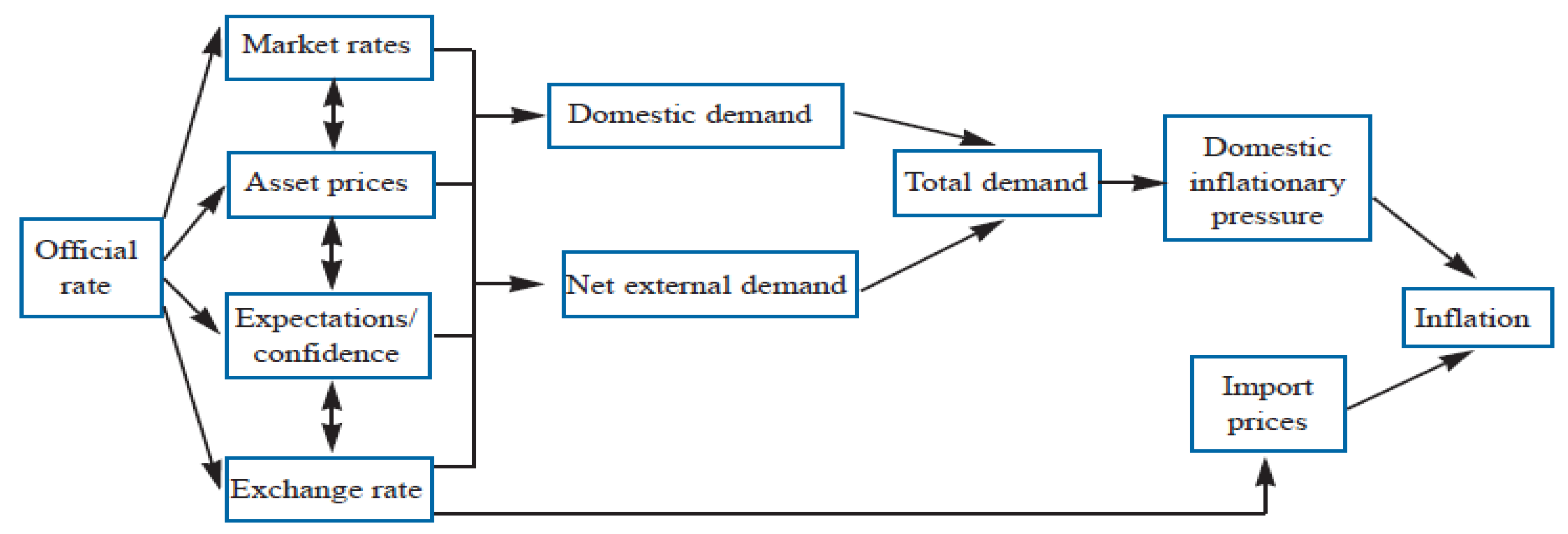
In constructing the macroeconomic uncertainty index, Jurado et al. (2015) assumed a rich data environment and employed over one hundred macroeconomic series. Then, they used principal component analysis to extract principal components that were used to forecast macroeconomic variables of interest. However, as demonstrated by Boivin and Ng (2006) and Koop and Korobilis (2014), using all available data to extract factors is not always optimal in principal component analysis. As mentioned, we divided macroeconomic uncertainty into activity uncertainty and inflation uncertainty. To select variables to predict economic activity and inflation, we used the Bank of England’s diagrammatic representation of the monetary policy transmission mechanism (June 2012).
As illustrated in Figure 1, monetary policy adjusts economic activity and inflation through financial markets. In the first stage, changes in monetary policy affects four groups of variables, namely market interest rates, asset prices, consumer and investor confidence and exchange rates, which in turn jointly influence economic activity. Then, inflation is affected by shifts in both economic activity and the foreign exchange market. Therefore, by defining macroeconomic uncertainty as the uncertainty in forecasting economic activity and in forecasting the inflation rate, we opted to use financial variables that are most relevant in monetary policy transmission in the estimation of macroeconomic uncertainty. In other words, instead of employing 147 financial time series as in Jurado et al. (2015), we concentrated on variables that are theoretically well justified in predicting economic activity and inflation. Table 1 lists 45 indicators under eight categories that were used in estimating our macroeconomic uncertainty indices.
In Table 1 (Panel A), we list eleven interest rates (source: Bank of England Interactive Database) and six bond yields (source: DataStream) to fully capture changes in market rates caused by shifts in monetary policy. Bond yields were also employed to forecast economic activity and inflation because they are the return an investor realises on fixed-income investment and should be highly correlated with the central bank’s interest rate. Table 1 (Panel B) presents five asset price indicators (source: DataStream) representing the primary types of assets in the market. As demonstrated by existing literature (e.g., Kiyotaki and Moore 1997) and the Monetary Policy Committee of the Bank of England (June 2012), changes in asset prices should signal changes in real GDP and the inflation rate. From an individual’s perspective, changes in asset prices affect financial wealth, which in turn affects consumption. From the perspective of a company, an increase (decrease) in its stock price should strengthen (weaken) its borrowing capacity by raising (reducing) the value of collateral which in turn has an impact on the company’s investment activities. All of the above changes in individuals’ and companies’ behaviour, when added up across the economy, generate changes in aggregate spending and economic activity. The three indices (source: DataStream) listed in Table 1 (Panel C) measure confidence and expectations of consumers, manufacturers and investors respectively who are the three primary market participants. Table 1 (Panel D) includes the exchange rate (source: Bank of England Interactive Database) between the UK and 15 of its top trading partners in terms of export sales in 2016. Exchange rate changes lead to changes in the relative prices of domestic and foreign goods and services and hence affect economic activity.
The use of variables listed in Table 1 (Panel A–D) is expected to describe the effect of monetary policy on real economic activity in normal circumstances. However, in certain periods such as the 2007–2009 financial crisis, the interest rate was reduced to the effective zero lower bound in the UK, and central bankers considered alternative instruments, for instance credit and money supply, to guide the economy. As described by Joyce et al. (2011), in response to the intensification of the financial crisis in autumn 2008, the Bank of England (BOE) loosened monetary policy using quantitative easing. Hence, credit and money also contain valuable information in forecasting the macroeconomic environment (Jurado et al. 2015). An increase in the supply of money and credit is usually associated with an improvement in economic activity. Therefore, we also used money supply indicators (as in Table 1 (Panel E), source: Bank of England Interactive Database) and lending indicators (listed in Table 1 (Panel F), source: DataStream) to support our prediction of economic activity and inflation. The inclusion of lending variables is in line with past literature (e.g., Hatzius et al. 2010; Koop and Korobilis 2014) as a measure of availability of finance.
Because some economic activity indicators including GDP are not available on a monthly basis, we used the growth rate of the real industrial production index (source: OECD) and the unemployment rate (source: Office for National Statistics) to measure real economic activity in the UK. Percentage changes in the retail price index, the producer price index and the consumer price index (source: DataStream) were employed as three inflation measures. In other words, we used the financial variables listed in Table 1 (Panel A–F) and the methodology discussed below to predict the five macroeconomic indicators in Table 1 (Panel G and H). The unforecastable components of the output indicators and that of the inflation indicators were considered as economics activity uncertainty (EAU) and inflation uncertainty (IU), respectively.
2.3. Economic Policy Uncertainty Indices
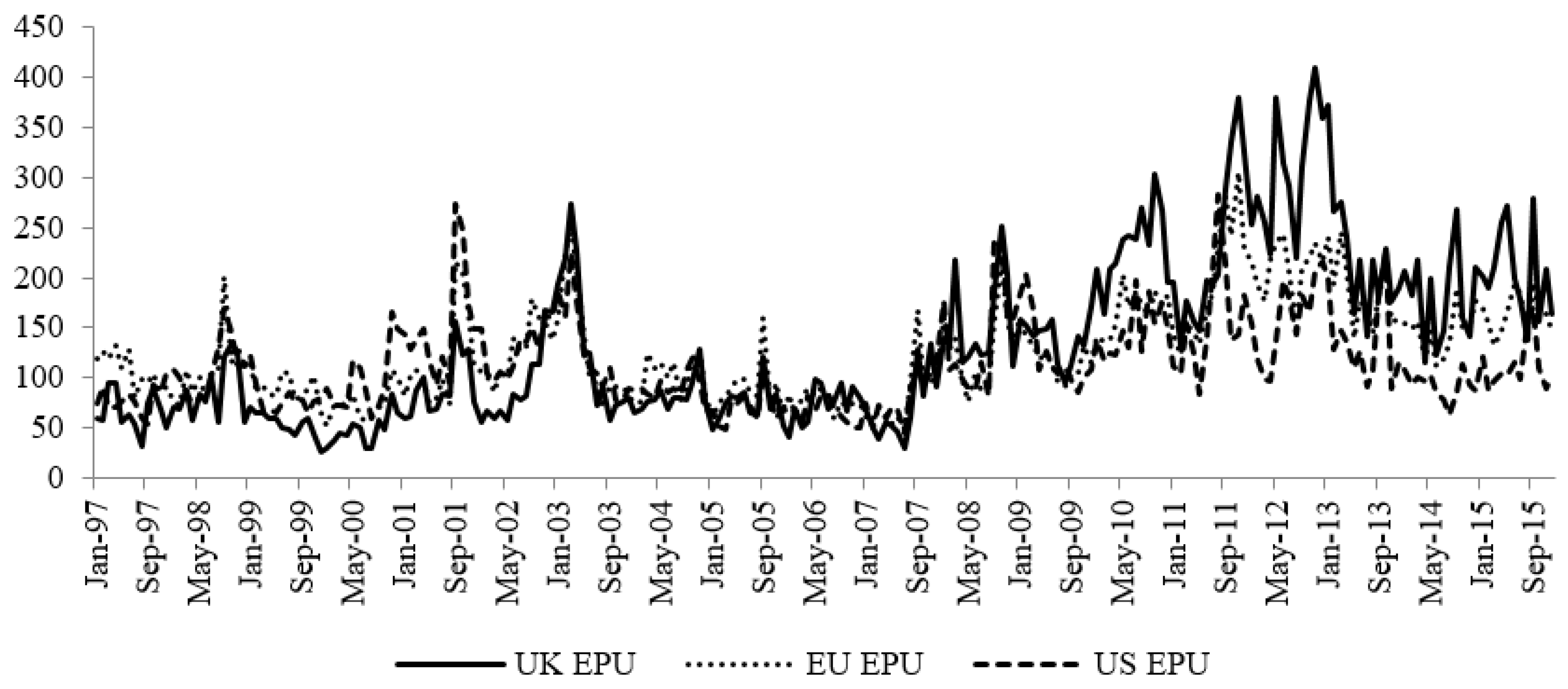
As already mentioned, in addition to investigating the pricing ability of output and inflation uncertainty, we were also interested in examining whether policy uncertainty can be used to price stocks return in the UK. We used three indices developed by Baker et al. (2016) and plotted in Figure 2 to measure economic policy uncertainty in the UK, the European Area and the US, respectively. Baker et al. (2016) developed the EPU index based on newspaper coverage frequency. They searched leading newspapers to obtain a monthly count of articles that contained the following trio of terms about: (i) the economy; (ii) policy; and (iii) uncertainty. An increase in their index indicates greater uncertainty in economic policy, which may harm macroeconomic performance.
3. Estimates of Macroeconomic Uncertainty
Rather than estimating uncertainty in each individual macroeconomic variable separately as in the study by Jurado et al. (2015), we used the heteroscedastic version of the Koop and Korobilis (2014) TVP-FAVAR model and calculated uncertainty jointly across variables. As mentioned above, the TVP-FAVAR model has the primary advantage over the traditional PCA of allowing the relationship between variables to vary over time. Following Koop and Korobilis (2014), we wrote a p-lag TVP-FAVAR model as follows:
where is an vector of normalised financial variables which are included in Table 1 (Panel A–F), is a vector of economic activity and inflation proxies in Table 1 (Panel G and H), represents loadings, , … are VAR parameters and both and are zero-mean Gaussian errors with covariances and , respectively. We set to ensure that the majority of the effect of monetary policy is transferred to economic activity and inflation. The term is the first principal component taking changes in the correlation structure between financial variables over time into account. Hatzius et al. (2010) considered extracting 1–3 factors using the PCA and discovered that the one-factor version performs as well as the other two versions.
Primiceri (2005), Del Negro and Otrok (2008) and Eickmeier et al. (2009) assumed a random walk process for and VAR parameters:
where . Primiceri (2005) and Nakajima (2011) supported stochastic volatility. Hence, we opted to let and be time-varying. As an identifying assumption in the existing literature (see, for instance, Primiceri 2005; Koop and Korobilis 2014), the covariance matrix was set to be diagonal, which ensures that is a vector of idiosyncratic shocks.
The system of Equations (2)–(5) constitutes a TVP-FAVAR model with stochastic volatility. Equation (2) extracts co-variation in a group of financial indicators that will be used in Equation (3) to predict . The disturbances of Equations (2) and (3) follow the normal distribution with time-varying volatilities and . It is worth reiterating that the TVP-FAVAR model developed thus far considers the likely changes in both parameters and loadings over time. Koop and Korobilis (2014) examined several versions of this model such as: (i) the factor-augmented VAR obtained from the TVP-FAVAR model under the restriction that both and are constant; (ii) the factor-augmented time-varying parameter VAR obtained from the TVP-FAVAR model under the constraint that the loadings are fixed; and (iii) the homoskedastic version of the TVP-FAVAR model by setting and . Among the different versions of the TVP-FAVAR model investigated, Koop and Korobilis (2014) showed that the “unconstrained” TVP-FAVAR model with stochastic volatility has the best performance in forecasting the macroeconomic variables in . In order words, the forecasting errors are minimised using the heteroscedastic version of the TVP-FAVAR.
Given our definition of macroeconomic uncertainty as the unforecastable component of output and inflation, the use of the Koop and Korobilis (2014) TVP-FAVAR model should produce the lowest macroeconomic uncertainty estimates. This means that estimated uncertainty based on other techniques (such as the traditional PCA used in Jurado et al. (2015)) may be over-estimated and thus contain an element which is actually forecastable. Due to the use of imperfect forecasting methods, many existing studies have included a proportion of forecastable components in the uncertainty index. This motivated us to use the TVP-FAVAR model that captures heteroscedasticity in order to forecast macroeconomic indicators in and estimate macroeconomic uncertainty. The reader is referred to Koop and Korobilis (2014) for their algorithm to estimate the system of Equations (2)–(5). It is worth noting that our sample of financial variables, as described in Table 1 (Panel A–F), is not balanced. For example, the sample period of the three-month Treasury bills discount rate started from January 2016 but the commercial paper rate was not available until March 2003. Following Koop and Korobilis (2014), was calculated only using the observed indicators at time .
As mentioned in Section 2, we used the industrial production index and the unemployment rate to measure economic activity and employed the retail price index, the producer price index and the customer price index to assess the price level. Rather than equally weighting all individual uncertainties as in the study by Jurado et al. (2015), we distinguished between the role of economic activity uncertainty () and inflation uncertainty (). We equally weighted the two resulting activity indices and the two resulting inflation indices as follows:
where , , , and denote unemployment uncertainty, industrial production uncertainty, RPI uncertainty, PPI uncertainty and CPI uncertainty, respectively. From Equation (1), the final five individual uncertainty indices are the absolute value of forecasting errors of Equation (3). The forecasting horizon was assumed to be six months (i.e., ). As demonstrated by Bali et al. (2016), the correlation coefficients between different uncertainty indices with different forecasting horizons are quite high and hence the choice of forecasting horizon should not affect the conclusion on uncertainty pricing.
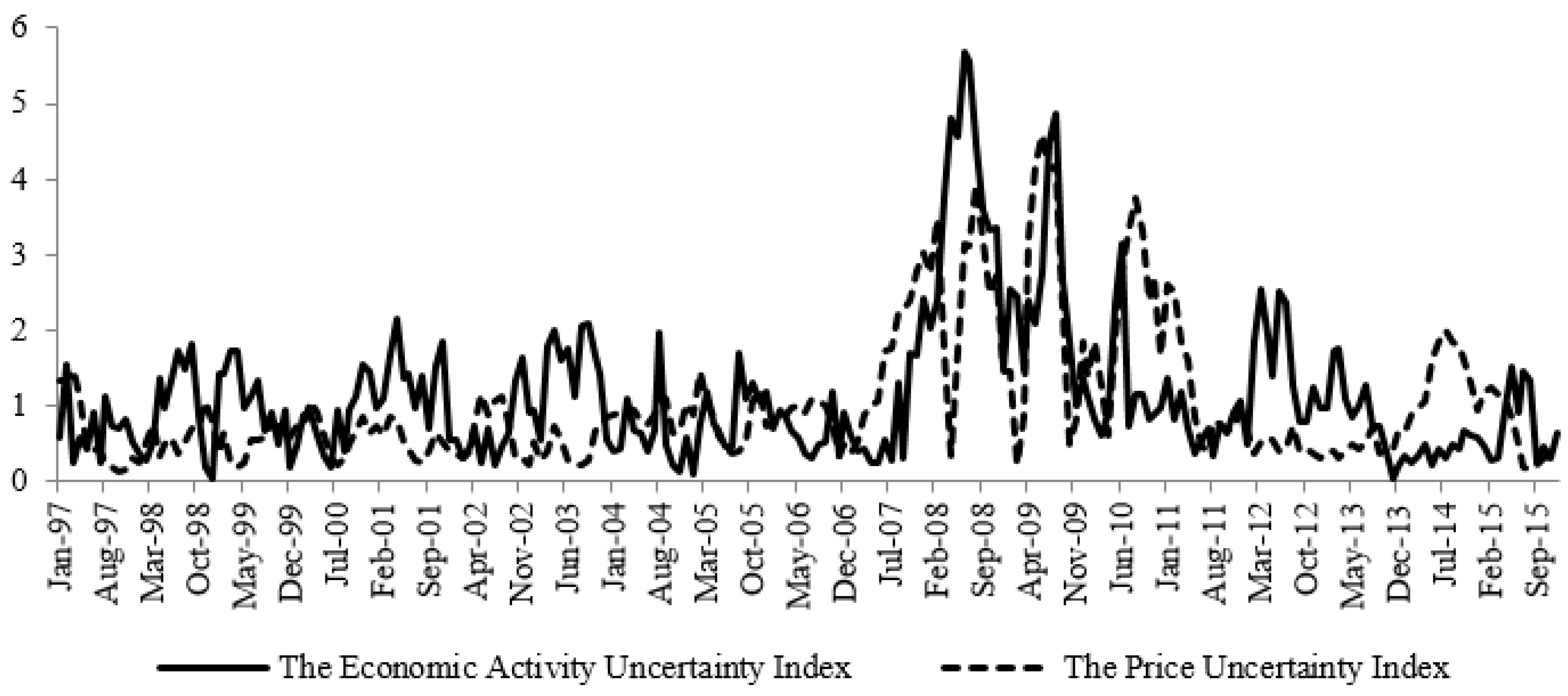
Our estimated uncertainty indices are displayed in Figure 3. Similar to the US economic uncertainty index provided by Jurado et al. (2015), both the economic activity uncertainty index and the inflation uncertainty index are generally high during the 2007–2009 financial crises. However, it is worth noting that the correlation coefficient between the two indices is about 0.466 which is relatively low and their movement is significantly different in some periods. For example, the economic activity uncertainty index rises considerably in 2012, but the inflation uncertainty index is relatively stable during the same year. Therefore, it is particularly interesting to distinguish the role of uncertainty in economic activity and in inflation in asset pricing. Taking the overall uncertainty index as the weighted average of all individual uncertainties as in the study by Jurado et al. (2015) may underestimate uncertainty in 2012, which in turn affects conclusions around the use of uncertainty in stock pricing.
4. Economic Uncertainty Pricing: The Method
We then investigated the role of economic uncertainty in pricing UK stocks. As mentioned above, we used three measures of economic uncertainty: (i) economic policy uncertainty; (ii) economic activity uncertainty; and (iii) inflation uncertainty. The measure of policy uncertainty was provided by Baker et al. (2016) based on newspaper coverage frequency, while the economic activity uncertainty index and the inflation uncertainty index were obtained as presented in Section 3 using the heteroscedastic version of the TVP-FAVAR model. Our stock sample includes all common stocks which were in the FTSE All Share Index historically.
In the first step, we constructed an economic uncertainty risk mimicking portfolio. For each measure of economic uncertainty (i.e., UK EPU, EU EPU, US EPU, EAU and IU), each month individual stock (excess) returns were regressed on the economic uncertainty measure as well as other benchmark factors for market, size, value, momentum and illiquidity risks. We estimated this OLS regression over the previous 36 months based on stocks with a minimum of 18 observations. Then, we sorted stocks into quantile portfolios according to their uncertainty risk, i.e., the coefficient (, uncertainty beta) on the measure of economic uncertainty:
where is the relevant economic uncertainty measure; is a matrix of other risk factors for market, size, value, momentum and illiquidity risks; and is the excess return of stock over the risk-free rate. The subscripts denote time. To construct our risk mimicking portfolios, we assigned stocks to a portfolio based on the estimated beta , which measures a stock’s sensitivity to the measure of economic uncertainty, in ascending order. It is worth noting that the value of may vary from negative to positive. In other words, Portfolio 1 contained stocks with the most negative while Portfolio 5 was constituted of stocks with the highest . As explained by Bali et al. (2016) using the US data, the portfolio with the most negative beta is associated with the highest risk of economic uncertainty and hence uncertainty-averse investors demand a premium in the form of higher expected return to hold this portfolio and vice versa. We calculated each portfolio return as the equally weighted average return of its constituent stocks for the following month. Portfolios were reformed monthly. The economic uncertainty risk mimicking portfolio was constructed as the difference between the “low minus high” portfolios (i.e., Quantile 1 minus Quantile 5).
In the second step, we estimated the alpha of the above risk mimicking portfolios in the following regression to examine whether the excess return of the low-beta portfolio over the high-beta portfolio can be explained by the existing risk factors (such as market, size, value, momentum and illiquidity risk factors).
or
where is the return on the low minus high portfolio; , j = 1, 2 … 6 are the risk factor loadings; and , , , , and are the returns on the benchmark factor portfolios for market, size, value, momentum, systematic illiquidity and characteristic illiquidity risks, respectively. Hence, is a measure of return adjusted by the aforementioned risks and can be used as a test statistic to evaluate the predictive power of uncertainty risk.
5. Empirical Results: Is Uncertainty Priced?
If UK stocks were exposed to economic uncertainty risk and if this risk were systematic, i.e., difficult to diversify, investors would require a premium for holding economic uncertainty sensitive stocks. Consistent with the recent study of Bali et al. (2016) using US data, our results provide some evidence that uncertainty is also priced into stock returns in the UK. The results presented in Table 2 and Table 3 were obtained using the Carhart (1997) four-factor model controlling for the market, size, value and momentum factors. In other words, we included four well-established risk factors (, , and ) in the matrix in Equation (8) while estimating stocks’ betas on economic uncertainty, , and used Equation (9) to estimate the alpha of the uncertainty risk mimicking portfolios, .
In Table 2 (Panel A), we report raw returns for the quantile portfolios and findings on whether UK economic policy uncertainty is priced in stock returns. We found that the top quantile portfolio (most negative ) tends to earn higher raw returns than the bottom quantile portfolio (most positive ) for stocks in the FTSE All Share index. Interestingly, the low minus high EPU risk quantile portfolios yields a four-factor alpha of 0.397% per month over the sample period (January 1997–December 2015)—significant at the 10% significance level.
These results relate to the broad group of FTSE All Share stocks. To investigate whether the above findings apply equally to stocks that are more commonly analysed and traded, we repeated the above analysis separately for the subset of FTSE 350 stocks and FTSE 100 stocks. In the third and fourth columns of Table 2 (Panel A), for the historic constituents of the FTSE 350 index and/or the FTSE 100 index, UK EPU is still priced in stock returns across Portfolios 1–5.
In Table 2 (Panel B and C), we present results from investigating whether economic policy uncertainty in the EU and US, respectively, plays a role in UK stock returns. Generally, there is little robust evidence in support of such a role: only domestic economic policy uncertainty is relevant.
Table 2 presents results around the pricing of economic policy uncertainty. Our study also examined the pricing of macroeconomic uncertainty, which was assessed by two factors in our study: economic activity uncertainty and inflation uncertainty. These results are given in Table 3. From Table 3 (Panel A), relating to economic activity uncertainty, it is quite clear that for FTSE All Share stocks, the alpha of the portfolio comprised of low minus high economic activity uncertainty stocks is significantly positive at least at the 5% significance level. However, there is no supporting evidence in the case of FTSE 350 and FTSE 100 stocks. In Table 3 (Panel B), relating to inflation uncertainty, we see very little evidence in support of a role for inflation uncertainty in UK stock returns.
Overall, Table 3 provides supporting evidence that stocks that are sensitive to fluctuations in UK economic activity command a future return premium. This is particularly the case for FTSE All Share stocks but not for the cross section of FTSE 350 and FTSE 100 stocks. However, the results fail to document a role for stocks’ sensitivity to inflation uncertainty in future stock returns. Therefore, although economic activity uncertainty and inflation uncertainty jointly contribute to the overall macroeconomic uncertainty, economic activity uncertainty is the real factor relating macroeconomic uncertainty variables to stock returns.
As previously mentioned, Foran et al. (2014, 2015) and Foran and O’Sullivan (2014, 2017) introduced two other risk factors, i.e., systematic and characteristic illiquidity risk factors, to price stock returns in the UK. For robustness purposes, we also investigated whether alphas estimated using either economic policy uncertainty or economic activity uncertainty can be explained by the Foran et al. (2014) illiquidity risk factors. Therefore, we recalculated the above results by introducing and as additional factors to the matrix in Equation (8) and used Equation (10) to estimate alphas of “low minus high” portfolios. Because our previous results indicate that none of EU Economic Policy Uncertainty, US Economic Policy Uncertainty and inflation uncertainty are priced in UK stock returns, we did not examine the role of these three indices. The results are presented in Table 4.
In Table 4 (Panel A), we are surprised to see that, for FTSE All Share stocks, the low minus high economic policy uncertainty sensitivity alpha was statistically insignificant. This indicates that the risk premium for economic policy uncertainty risk reported in Table 2 is explained by illiquidity risk factors. However, moving to FTSE 350 and FTSE 100 stocks that are more commonly traded and exhibit less illiquidity risk, we obtained strong evidence indicating that, controlling for both systematic and characteristic illiquidity risk factors together with the market, size, value and momentum factors, economic policy uncertainty in the UK is still priced into stock returns. The alpha of Portfolios 1–5 is significant at least at the 5% significance level. In Table 4 (Panel B), in the case of economic activity uncertainty pricing, there remains some, albeit weaker, evidence of a role for economic activity uncertainty in pricing among the broad universe of stocks. This is strongest in the case of FTSE 350 stocks (significant at the 5% significance level in the case of Portfolios 1–5). Therefore, the evidence indicates that our economic activity uncertainty risk factor plays some role in UK stock returns even controlling for all the existing risk factors in Foran et al. (2014).
Across all tabulated results, the emerging theme is that one-period ahead UK stock returns may be partly predicted by stocks’ sensitivity to UK economic policy uncertainty and UK economic activity uncertainty over the previous three years. This finding is particularly robust among FTSE 350 stocks, where it persists even after controlling for illiquidity risk factors in addition to more conventional risk factors for market, size, value and momentum risks.
6. Conclusions
We examined the role of economic uncertainty in explaining the cross-sectional variation of UK stock returns. We distinguished between economic activity and inflation uncertainty by employing five separate economic uncertainty indices. We also considered economic policy uncertainty. Our study is distinguished in particular by using financial variables that are theoretically justified in forecasting the economy to construct economic activity and inflation uncertainty indices for the UK. This is quite important because using all available information is not always optimal in predicting developments in the macro economy. After controlling for market, size, book-to-market and momentum and illiquidity risk factors, we found evidence in support of using our estimated activity uncertainty index and the Baker et al. (2016) UK economic policy uncertainty index to predict the cross-sectional variation of UK stock returns.
Our results suggest that stocks’ sensitivity to both UK inflation uncertainty and foreign economic policy uncertainty is not rewarded by higher returns. UK stock market investors should concentrate on stocks that are negatively sensitive to economic activity uncertainty and/or UK economic policy uncertainty to earn an abnormal return. From the policy perspective, regulators and policy makers may consider methods that are effective in reducing policy uncertainty and uncertainty in future economic growth. These include improving transparency of the policy making process and frequent publication of economic assessments, which may in turn encourage stock market development.
Author Contributions
J.G., S.Z., N.O. and M.S. conceived and designed the experiments; J.G. and S.Z. performed the experiments and analysed the data; J.G., S.Z., N.O. and M.S. discussed results and analytical methods; J.G., S.Z., N.O. and M.S. wrote the paper.
Funding
This research received no external funding.
Conflicts of Interest
The authors declare no conflicts of interest.
References
- Bake, Scott R., Nicholas Bloom, and Steven J. Davis. 2016. Measuring Economic Policy Uncertainty. Quarterly Journal of Economics 131: 1593–636. [Google Scholar] [CrossRef]
- Bali, Turan G., Stephen J. Brown, and Yi Tang. 2016. Is Economic Uncertainty Priced in the Cross-Section of Stock Returns? Georgetown McDonough School of Business Research Paper No. 2812967; Gabelli School of Business, Fordham University Research Paper No. 2812967. Available online: https://ssrn.com/abstract=2812967 (accessed on 5 January 2017).
- Bianchi, Francesco, Cosmin L. Ilut, and Martin Schneider. 2014. Uncertainty Shocks, Asset Supply and Pricing over the Business Cycle; NBRE Working Paper Series No. 20081. Cambridge: National Bureau of Economic Research.
- Bloom, Nicholas. 2009. The Impact of Uncertainty Shocks. Econometrica 77: 623–85. [Google Scholar]
- Boivin, Jean, and Serena Ng. 2006. Are More Data Always Better for Factor Analysis? Journal of Econometrics 132: 169–94. [Google Scholar] [CrossRef]
- Campbell, John Y. 1993. Intertemporal Asset Pricing without Consumption Data. American Economic Review 83: 487–512. [Google Scholar]
- Campbell, John Y. 1996. Understanding Risk and Return. Journal of Political Economy 104: 298–345. [Google Scholar] [CrossRef] [Green Version]
- Carhart, Mark M. 1997. On Persistence in Mutual Fund Performance. Journal of Finance 52: 57–82. [Google Scholar] [CrossRef] [Green Version]
- Chen, Zengjing, and Larry G. Epstein. 2002. Ambiguity, Risk, and Asset Returns in Continuous Time. Econometrica 70: 1403–45. [Google Scholar] [CrossRef]
- Del Negro, Marco, and Christopher Otrok. 2008. Dynamic Factor Models with Time-Varying Parameters: Measuring Changes in International Business Cycles. Federal Reserve Bank of New York Staff Reports No. 326. New York: Federal Reserve Bank. [Google Scholar]
- Eickmeier, Sandra, Wolfgang Lemke, and Massimiliano Marcellino. 2009. Classical Time-Varying FAVAR Models—Estimation, Forecasting and Structural Analysis. Discussion Paper Series 1: Economic Studies No. 04/2011. Frankfurt: Deutsche Bundesbank. [Google Scholar]
- Ellsberg, Daniel. 1961. Risk, Ambiguity, and the Savage Axioms. Quarterly Journal of Economics 75: 643–69. [Google Scholar] [CrossRef]
- Epstein, Larry G., and Martin Schneider. 2010. Ambiguity and Asset Markets. Annual Reviews of Financial Economics 2: 315–34. [Google Scholar] [CrossRef]
- Epstein, Larry G., and Tan Wang. 1994. Intertemporal Asset Pricing under Knightian Uncertainty. Econometrica 57: 937–69. [Google Scholar] [CrossRef]
- Fama, Eugene F., and Kenneth R. French. 1993. Common Risk Factors in the Returns on Stocks and Bonds. Journal of Financial Economics 33: 3–56. [Google Scholar] [CrossRef]
- Fama, Eugene F., and Kenneth R. French. 2015. A Five-factor Asset Pricing Model. Journal of Financial Economics 116: 1–22. [Google Scholar] [CrossRef]
- Federal Open Market Committee. 2009. Minutes of the December (2009) Meeting. Available online: http://www.federalreserve.gov/monetarypolicy/fomcminutes20091216.htm (accessed on 11 January 2017).
- Foran, Jason, and Niall O’Sullivan. 2014. Liquidity Risk and the Performance of UK Mutual Funds. International Review of Financial Analysis 35: 178–89. [Google Scholar] [CrossRef]
- Foran, Jason, and Niall O’Sullivan. 2017. Mutual Fund Skill in Timing Market Volatility and Liquidity. International Journal of Finance and Economics 22: 257–73. [Google Scholar] [CrossRef]
- Foran, Jason, Mark C. Hutchinson, and Niall O’Sullivan. 2014. The Asset Pricing Effects of UK Market Liquidity Shocks: Evidence from Tick Data. International Review of Financial Analysis 32: 85–94. [Google Scholar] [CrossRef]
- Foran, Jason, Mark C. Hutchinson, and Niall O’Sullivan. 2015. Liquidity Commonality and Pricing in UK Equities. Research in International Business and Finance 34: 281–93. [Google Scholar] [CrossRef]
- Gomes, Joao, Leonid Kogan, and Lu Zhang. 2003. Equilibrium Cross Section of Returns. Journal of Political Economy 117: 941–86. [Google Scholar] [CrossRef]
- Gregory, Alan, Rajesh Tharyan, and Angela Christidis. 2013. Constructing and Testing Alternative Versions of the Fama-French and Carhart Models in the UK. Journal of Business Finance and Accounting 40: 172–214. [Google Scholar] [CrossRef] [Green Version]
- Hatzius, Jan, Peter Hooper, Frederic S. Mishkin, Kermit L. Schoenholtz, and Mark W. Watson. 2010. Financial Condition Indexes: A Fresh Look after the Financial Crisis. NBER Working Paper Series No. 16150. Cambridge: National Bureau of Economic Research. [Google Scholar]
- Hou, Kewei, Chen Xue, and Lu Zhang. 2015. Digesting Anomalies: An Investment Approach. Review of Financial Studies 28: 650–705. [Google Scholar] [CrossRef]
- International Monetary Fund. 2012. World Economic Outlook: Coping with High Debt and Sluggish Growth. Washington, DC: IMF Press. [Google Scholar]
- International Monetary Fund. 2013. World Economic Outlook: Hopes, Realities, Risks. Washington, DC: IMF Press. [Google Scholar]
- Jensen, Michael C. 1968. The Performance of Mutual Funds in the Period 1945–1964. Journal of Finance 23: 389–416. [Google Scholar] [CrossRef]
- Joyce, Michael, Matthew Tong, and Robert Woods. 2011. The United Kingdom’s Quantitative Easing Policy: Design, Operation and Impact. Quarterly Bulletin. London: Bank of England. [Google Scholar]
- Jurado, Kyle, Sydney C. Ludvigson, and Serena Ng. 2015. Measuring Uncertainty. American Economic Review 105: 1177–216. [Google Scholar] [CrossRef]
- Kiyotaki, Nobuhiro, and John Moore. 1997. Credit Cycles. Journal of Political Economy 105: 211–48. [Google Scholar] [CrossRef]
- Koop, Gary, and Dimitris Korobilis. 2014. A New Index of Financial Conditions. European Economics Review 71: 101–16. [Google Scholar] [CrossRef]
- Merton, Robert C. 1973. An Intertemporal Capital Asset Pricing Model. Econometrica 41: 867–87. [Google Scholar] [CrossRef]
- Monetary Policy Committee. 2012. The Transmission Mechanism of Monetary Policy. Available online: http://www.bankofengland.co.uk/publications/Documents/other/monetary/montrans.pdf (accessed on 31 March 2014).
- Nakajima, Jouchi. 2011. Time-varying Parameter VAR Model with Stochastic Volatility: An Overview of Methodology and Empirical Applications. Monetary and Economic Studies 29: 107–42. [Google Scholar]
- Pastor, Lubos, and Robert F. Stambaugh. 2003. Liquidity Risk and Expected Stock Returns. Journal of Political Economy 111: 642–85. [Google Scholar] [CrossRef]
- Primiceri, Giorgio E. 2005. Time Varying Structural Vector Autoregressions and Monetary Policy. Review of Economic Studies 72: 821–52. [Google Scholar] [CrossRef]
| 1 | The well-known risk factors considered in the Jurado et al. (2015) study are the market, size, book-to-market, momentum, liquidity, investment and profitability factors of Fama and French (1993, 2015), Carhart (1997), Pastor and Stambaugh (2003) and Hou et al. (2015). |
| 2 | A detailed discussion is provided in Section 2. |
Figure 1.
The transmission mechanism of monetary policy. Source: Monetary Policy Committee (2012), p. 3.
Figure 1.
The transmission mechanism of monetary policy. Source: Monetary Policy Committee (2012), p. 3.

Figure 2.
The economic policy uncertainty indices, 1997–2015. Source: Baker et al. (2016).
Figure 2.
The economic policy uncertainty indices, 1997–2015. Source: Baker et al. (2016).

Figure 3.
Macroeconomic uncertainty indices, 1997–2015.


Table 1.
Classification of financial and macroeconomic indicators.
| Name | Description |
|---|---|
| Panel A: Market Interest Rates and Bond Yields | |
| 1. Trea3m | Monthly average of three-month Treasury bills discount rate, Sterling |
| 2. Elig3m | Monthly average of Eligible bills’ discount rate, 3 months |
| 3. BankRate | Monthly average of UK Banks’ base rates |
| 4. EuDepo | Monthly average of 3-month Euro-currency deposit rate |
| 5. Gil3m | Monthly average of Gilt repo interest rate, 3 months |
| 6. Comm3m | Monthly average of Euro-commercial paper rate, 3 months, Sterling |
| 7. EuBills | Monthly average of BOE 3-month Euro bills’ discount rate |
| 8. Sonia | Monthly average of Sterling overnight index average interbank lending rate |
| 9. Cert3m | Monthly average of Sterling certificates of deposit interest rate, 3 months |
| 10. SecRate | Financial institutions sterling 2-year variable rate mortgage to households |
| 11. UnsecRate | Interest rate of UK monetary financial institutions sterling Personal loan |
| 12. Corp10yr | Monthly average of FTSE Sterling corporate bond yields, 10 year+ |
| 13. CorpFin | Monthly average of FTSE Sterling corporate bond yields, financial sector |
| 14. CorpAll | Monthly average of FTSE Sterling corporate bond yields, all maturities |
| 15. CorpBBB | Monthly average of FTSE Sterling corporate bond yields, BBB rated |
| 16. CorpAA | Monthly average of FTSE Sterling corporate bond yields, AA rated |
| 17. Gov10yr | Monthly average of the UK Benchmark 10 yr Datastream Gov. Index |
| Panel B: Asset Prices | |
| 18. GPI | Monthly average of the gold price in Sterling |
| 19. HPI | Monthly average of the Halifax House Price Index, seasonally adjusted |
| 20. SPI | Monthly average of the FTSE All share index |
| 21. CmPI | Monthly average of the Reuters commodity index, Sterling |
| 22. OPI | Monthly average of OPEC oil basket price US$ per Bbl |
| Panel C: Confidence and Expectations | |
| 23. CCI | UK GFK Consumer confidence index, monthly average |
| 24. IndCI | Industry Survey, Total Manufacturing, Industrial Confidence Indicator |
| 25. InvCI | State Street European investor confidence index, monthly average |
| Panel D: Exchange Rates (with Top 15 Major Trading Partners) | |
| 26. Yuan | Chinese Yuan against Sterling, monthly average |
| 27. Can$ | Canadian Dollar against Sterling, monthly average |
| 28. Euro | Euro against Sterling, monthly average |
| 29. HK$ | Hong Kong Dollar against Sterling, monthly average |
| 30. Yen | Japanese Yen against Sterling, monthly average |
| 31. Franc | Swiss Franc against Sterling, monthly average |
| 32. Krona | Swedish Krona against Sterling, monthly average |
| 33. Riyal | Saudi Riyal against Sterling, monthly average |
| 34. US$ | US Dollar against Sterling, monthly average |
| Panel E: Money Supply | |
| 35. M1gr | Monthly changes in M1, seasonally adjusted |
| 36. M2gr | Monthly changes in M2, seasonally adjusted |
| 37. M3gr | Monthly changes in M3, seasonally adjusted |
| 38. M4gr | Monthly changes in M4, seasonally adjusted |
| Panel F: Financial Institutions’ Lending | |
| 39. UnseLend | Monthly changes in UK net unsecured lending to individuals |
| 40. MortLend | Monthly changes in mortgage lending by UK lenders for house purchase |
| Panel G: Economic Activity Indicators | |
| 41. IPXgr | The growth rate of industrial production index (chained volume measures) |
| 42. Unem | The unemployment rate (aged 16 and over, seasonally adjusted) |
| Panel H: Inflation Indicators | |
| 43. RPI | RPI All Items: Percentage change over 12 months |
| 44. PPI | PPI All Manufactured Products: Percentage change over 12 months |
| 45. CPI | CPI All Items: Percentage change over 12 months |
Source: Bank of England, Interactive Database and DataStream.
Table 2.
Pricing of uncertainty: economic policy uncertainty.
| FTSE All Share | FTSE 350 | FTSE 100 | |
|---|---|---|---|
| Panel A: UK Economic Policy Uncertainty | |||
| Raw Return, %: Quantile 1 | 0.763 | 0.788 | 0.564 |
| Raw Return, %: Quantile 2 | 0.611 | 0.635 | 0.335 |
| Raw Return, %: Quantile 3 | 0.541 | 0.555 | 0.434 |
| Raw Return, %: Quantile 4 | 0.453 | 0.522 | 0.452 |
| Raw Return, %: Quantile 5 | 0.438 | 0.272 | 0.076 |
| Alpha, %: Portfolios 1–5 | 0.397 * | 0.615 *** | 0.479 * |
| (0.0650) | (0.0039) | (0.0981) | |
| Panel B: EU Economic Policy Uncertainty | |||
| Raw Return, %: Quantile 1 | 0.682 | 0.657 | 0.538 |
| Raw Return, %: Quantile 2 | 0.620 | 0.624 | 0.516 |
| Raw Return, %: Quantile 3 | 0.555 | 0.570 | 0.372 |
| Raw Return, %: Quantile 4 | 0.567 | 0.540 | 0.195 |
| Raw Return, %: Quantile 5 | 0.325 | 0.348 | 0.154 |
| Alpha, %: Portfolios 1–5 | 0.399 * | 0.381 * | 0.319 |
| (0.0511) | (0.0607) | (0.2037) | |
| Panel C: US Economic Policy Uncertainty | |||
| Raw Return, %: Quantile 1 | 0.679 | 0.545 | 0.450 |
| Raw Return, %: Quantile 2 | 0.611 | 0.652 | 0.479 |
| Raw Return, %: Quantile 3 | 0.531 | 0.593 | 0.318 |
| Raw Return, %: Quantile 4 | 0.519 | 0.551 | 0.464 |
| Raw Return, %: Quantile 5 | 0.424 | 0.380 | 0.062 |
| Alpha, %: Portfolios 1–5 | 0.296 | 0.108 | 0.270 |
| (0.2317) | (0.6190) | (0.3091) | |
Note: For all stocks in the FTSE All Share index, the FTSE 350 index or the FTSE 100 index, each month economic uncertainty risk for stock i was estimated by regressing stock i’s returns over the previous 36 months on the Baker et al. (2016) EPU index along with market, size, value and momentum factors. A stock’s economic uncertainty risk is the beta on the EPU index. Stocks were sorted into five equal weighted portfolios based on beta and held for one month before reforming the portfolios. The time series of the low-uncertainty beta portfolio minus the high-uncertainty beta portfolio was tested against the Carhart (1997) four-factor model. Table 2 reports the alphas of these regressions with p-values in parentheses. * represents significance at 10%, ** represents significance at 5% and *** represents significance at 1%.
Table 3.
Pricing of uncertainty: inflation and economic activity uncertainty.
| FTSE All Share | FTSE 350 | FTSE 100 | |
|---|---|---|---|
| Panel A: Economic Activity Uncertainty | |||
| Raw Return, %: Quantile 1 | 0.619 | 0.573 | 0.283 |
| Raw Return, %: Quantile 2 | 0.661 | 0.732 | 0.400 |
| Raw Return, %: Quantile 3 | 0.645 | 0.619 | 0.610 |
| Raw Return, %: Quantile 4 | 0.531 | 0.515 | 0.392 |
| Raw Return, %: Quantile 5 | 0.217 | 0.276 | 0.049 |
| Alpha, %: Portfolios 1–5 | 0.486 ** | 0.302 | 0.034 |
| (0.0184) | (0.1740) | (0.9183) | |
| Panel B: Inflation Uncertainty | |||
| Raw Return, %: Quantile 1 | 0.511 | 0.474 | 0.333 |
| Raw Return, %: Quantile 2 | 0.662 | 0.785 | 0.553 |
| Raw Return, %: Quantile 3 | 0.565 | 0.528 | 0.327 |
| Raw Return, %: Quantile 4 | 0.544 | 0.530 | 0.301 |
| Raw Return, %: Quantile 5 | 0.429 | 0.400 | 0.230 |
| Alpha, %: Portfolios 1–5 | 0.081 | 0.042 | 0.158 |
| (0.6889) | (0.8546) | (0.5238) | |
Note: For all stocks in the FTSE All Share index, the FTSE 350 index or the FTSE 100 index, each month economic uncertainty risk for stock i was estimated by regressing stock i’s returns over the previous 36 months on the macroeconomic uncertainty index (economic activity uncertainty or inflation uncertainty) along with market, size, value and momentum factors. A stock’s economic uncertainty risk is the beta on the macroeconomic uncertainty index. Stocks were sorted into five equal weighted portfolios based on beta and held for one month before reforming the portfolios. The time series of the low-uncertainty beta portfolio minus the high-uncertainty beta portfolio was tested against the Carhart (1997) four-factor model. Table 3 reports the alphas of these regressions with p-values in parentheses. * represents significance at 10%, ** represents significance at 5% and *** represents significance at 1%.
Table 4.
Pricing of economic uncertainty.
| FTSE All Share | FTSE 350 | FTSE 100 | |
|---|---|---|---|
| Panel A: UK Economic Policy Uncertainty | |||
| Raw Return, %: Quantile 1 | 0.855 | 0.724 | 0.565 |
| Raw Return, %: Quantile 2 | 0.561 | 0.611 | 0.282 |
| Raw Return, %: Quantile 3 | 0.564 | 0.590 | 0.309 |
| Raw Return, %: Quantile 4 | 0.410 | 0.534 | 0.668 |
| Raw Return, %: Quantile 5 | 0.529 | 0.370 | 0.067 |
| Alpha, %: Portfolios 1–5 | 0.381 | 0.903 *** | 0.998 ** |
| (0.2218) | (0.0000) | (0.0127) | |
| Panel B: Economic Activity Uncertainty | |||
| Raw Return, %: Quantile 1 | 0.607 | 0.613 | 0.274 |
| Raw Return, %: Quantile 2 | 0.642 | 0.680 | 0.437 |
| Raw Return, %: Quantile 3 | 0.666 | 0.573 | 0.467 |
| Raw Return, %: Quantile 4 | 0.521 | 0.528 | 0.466 |
| Raw Return, %: Quantile 5 | 0.370 | 0.426 | 0.139 |
| Alpha, %: Portfolios 1–5 | 0.441 * | 0.548 ** | 0.483 |
| (0.0835) | (0.0408) | (0.2495) | |
Note: For all stocks in the FTSE All Share index, the FTSE 350 index or the FTSE 100 index, each month economic uncertainty risk for stock i was estimated by regressing stock i’s returns over the previous 36 months on the economic uncertainty index (the UK EPU index or the economic activity uncertainty index) along with market, size, value, momentum and illiquidity factors. A stock’s economic uncertainty risk is the beta on the economic uncertainty index. Stocks were sorted into five equal weighted portfolios based on beta and held for one month before reforming the portfolios. The time series of the low-uncertainty beta portfolio minus the high-uncertainty beta portfolio was tested against the Foran et al. (2014) five-factor model. Table 4 reports the alphas of these regressions with p-values in parentheses. * represents significance at 10%, ** represents significance at 5% and *** represents significance at 1%.
© 2019 by the authors. Licensee MDPI, Basel, Switzerland. This article is an open access article distributed under the terms and conditions of the Creative Commons Attribution (CC BY) license (http://creativecommons.org/licenses/by/4.0/).
Share and Cite
MDPI and ACS Style
Gao, J.; Zhu, S.; O’Sullivan, N.; Sherman, M. The Role of Economic Uncertainty in UK Stock Returns. J. Risk Financial Manag. 2019, 12, 5. https://doi.org/10.3390/jrfm12010005
AMA Style
Gao J, Zhu S, O’Sullivan N, Sherman M. The Role of Economic Uncertainty in UK Stock Returns. Journal of Risk and Financial Management. 2019; 12(1):5. https://doi.org/10.3390/jrfm12010005
Chicago/Turabian StyleGao, Jun, Sheng Zhu, Niall O’Sullivan, and Meadhbh Sherman. 2019. "The Role of Economic Uncertainty in UK Stock Returns" Journal of Risk and Financial Management 12, no. 1: 5. https://doi.org/10.3390/jrfm12010005