Bank Credit and Housing Prices in China: Evidence from a TVP-VAR Model with Stochastic Volatility


Abstract

1. Introduction
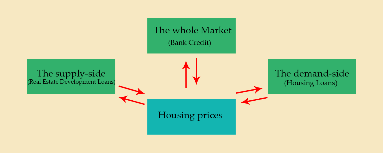
2. Theoretical Analysis of the Interaction Effect between Bank Credit and Housing Prices
3. Time-Varying Parameter VAR Model with Stochastic Volatility
4. Data and Settings
5. Empirical Results
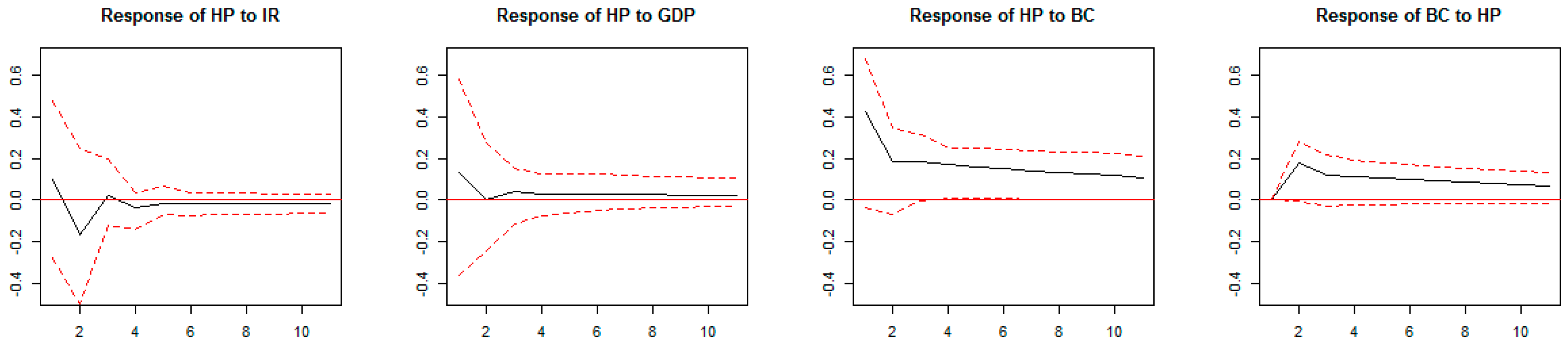
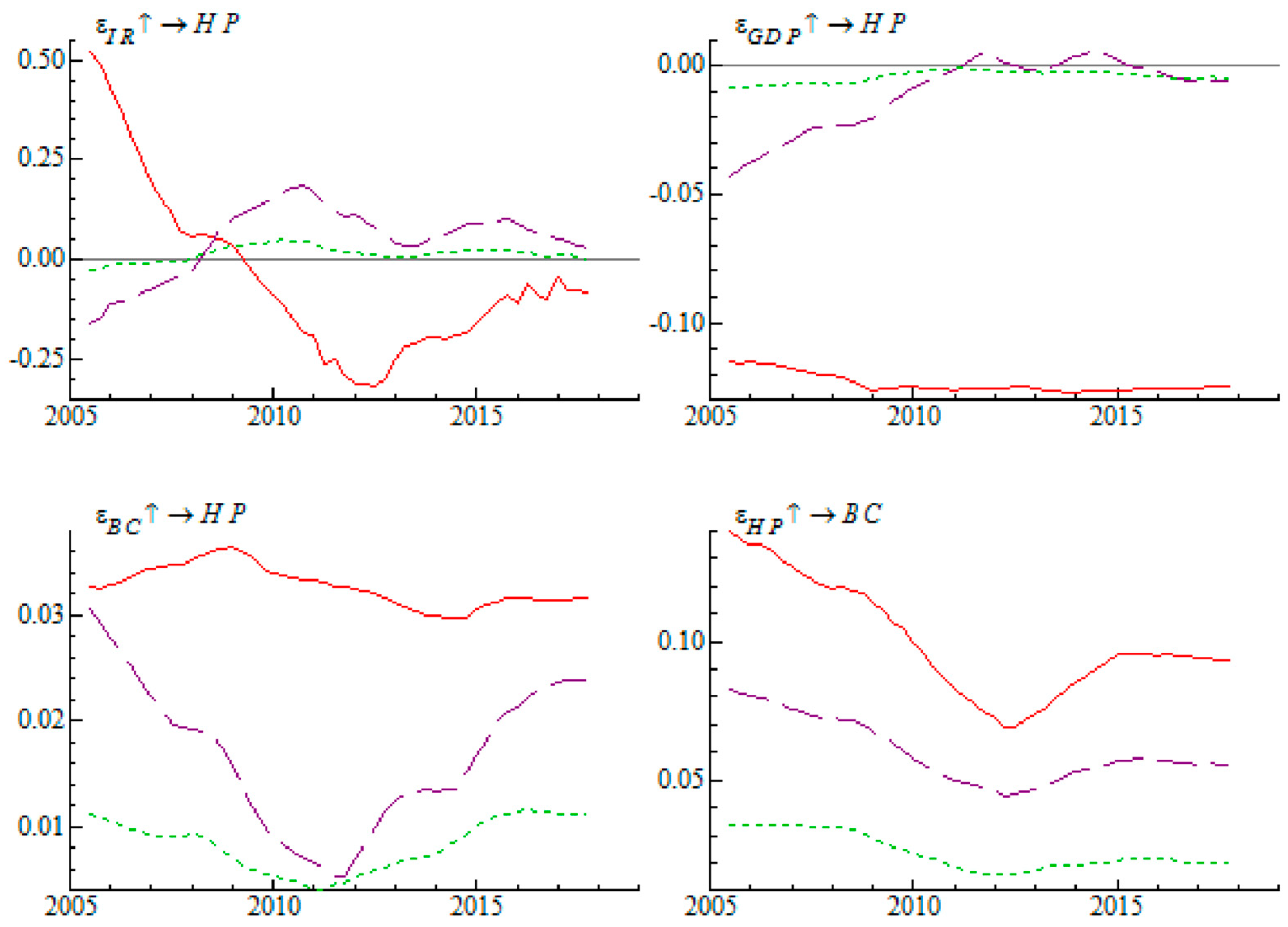
5.1. Bank Credit and Housing Prices
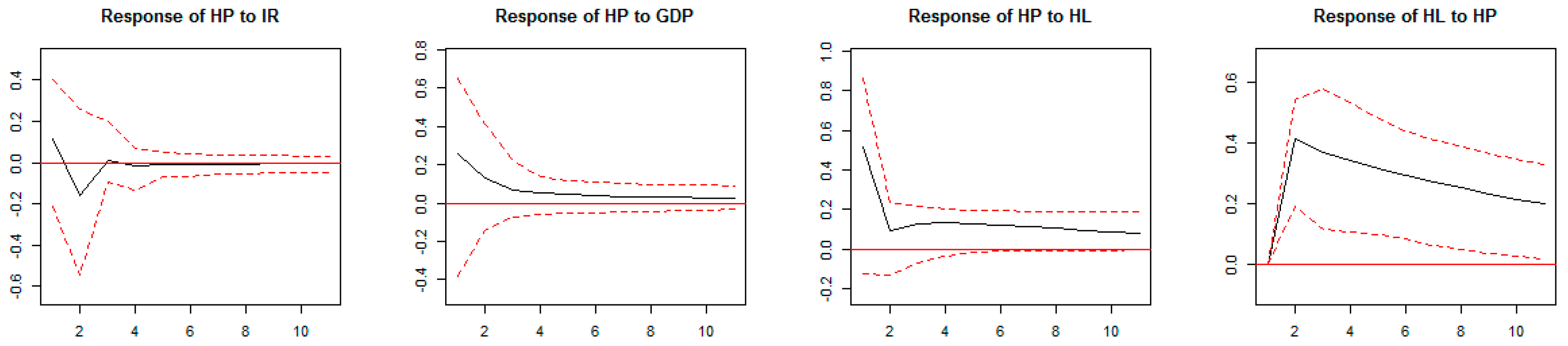
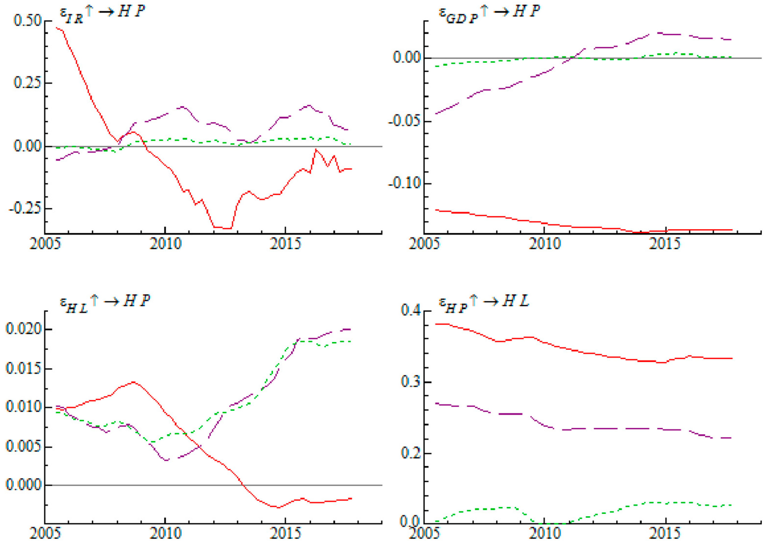
5.2. Housing Loans and Housing Prices
5.3. Real Estate Development Loan and Housing Prices
6. Conclusions
Author Contributions
Funding
Acknowledgments
Conflicts of Interest
References
- Black, Fischer. 1976. Studies of Stock Market Volatility Changes. In Proceedings of the 1976 Meetings of the Business and Economic Statistics Section. Washington DC: American Statistical Association, pp. 177–81. [Google Scholar]
- Cai, Weina, and Sen Wang. 2018. The Time-Varying Effects of Monetary Policy on Housing Prices in China: An Application of TVP-VAR Model with Stochastic Volatility. International Journal of Business Management 13: 149–57. [Google Scholar] [CrossRef]
- Collyns, Charles, and Abdelhak Senhadji. 2002. Lending Booms, Real Estate, and The Asian Crisis. IMF Working Paper. Washington DC: IMF, pp. 1–46. Available online: https://ssrn.com/abstract=879360 (accessed on 10 September 2018).
- Davis, E. Philip, and Haibin Zhu. 2011. Bank lending and commercial property cycles: Some cross-country evidence. Journal of International Money and Finance 30: 1–21. [Google Scholar] [CrossRef]
- David, Nissim Ben. 2013. Predicting housing prices according to expected future interest rate. Applied Economics 45: 3044–48. [Google Scholar] [CrossRef]
- Geweke, John. 1992. Evaluating the Accuracy of Sampling-Based Approaches to the Calculation of Posterior Moments. In Bayesian Statistics 4. Edited by José-Miguel Bernardo, James O. Berger, Alexander Philip Dawid and Adrian Frederick Melhuish Smith. Oxford: Oxford University Press, pp. 169–93. [Google Scholar]
- Gerlach, Stefan, and Wensheng Peng. 2005. Bank Lending and Property Prices in Hong Kong. Journal of Banking & Finance 29: 461–81. [Google Scholar] [CrossRef]
- Goodhart, Charles, and Boris Hofmann. 2008. House Prices, Money, Credit and the Macroeconomy. Oxford Review of Economic Policy 24: 180–205. Available online: https://EconPapers.repec.org/RePEc:oup:oxford:v:24:y:2008:i:1:p:180-205 (accessed on 20 October 2018). [CrossRef]
- Gimeno, Ricardo, and Carmen Martínez Carrascal. 2010. The relationship between house prices and house purchase loans: The Spanish case. Journal of Banking & Finance 34: 1849–55. [Google Scholar] [CrossRef]
- Hong, Liming. 2014. The Dynamic Relationship between Real Estate Investment and Economic Growth: Evidence from Prefecture City Panel Data in China. IERI Procedia 7: 2–7. [Google Scholar] [CrossRef]
- McQuinn, Kieran, and Gerard O’Reilly. 2008. Assessing the role of income and interest rates in determining house prices. Economic Modelling 25: 377–90. [Google Scholar] [CrossRef]
- Mwabutwa, Chance, Nicola Viegi, and Manoel Bittencourt. 2016. Evolution of Monetary Policy Transmission Mechanism in Malawi: A TVP-VAR Approach. Journal of Economic Development 41: 33–55. [Google Scholar]
- Mora, Nada. 2008. The Effect of Bank Credit on Asset Prices: Evidence from the Japanese Real Estate Boom during the 1980s. Journal of Money, Credit and Banking 40: 57–87. Available online: https://www.jstor.org/stable/25096240 (accessed on 19 September 2018). [CrossRef]
- Nakajima, Jouchi. 2011. Time-Varying Parameter VAR Model with Stochastic Volatility: An Overview of Methodology and Empirical Applications. IMES Discussion Paper Series, 11-E-09; Tokyo: Institute for Monetary and Economic Studies, Bank of Japan. [Google Scholar]
- Primiceri, Giorgio. 2005. Time Varying Structural Vector Autoregressions and Monetary Policy. The Review of Economic Studies 72: 821–52. [Google Scholar] [CrossRef]
- Qin, Lin, and Yimin Yao. 2012. A Study of the Relationship between Bank Credit and Real Estate Prices. Comparative Economic & Social Systems 2: 188–202. (In Chinese). [Google Scholar]
- Shephard, Neil. 1996. Statistical Aspects of ARCH and Stochastic Volatility. In Time Series Models in Econometrics, Finance and Other Fields. London: Chapman & Hall, pp. 1–67. [Google Scholar]
- Taylor, Stephen J. 1986. Modelling Financial Time Series. Chichester: John Wiley. [Google Scholar]
- Tian, Shuairu, and Shigeyuki Hamori. 2016. Time-Varying Price Shock Transmission and Volatility Spillover in Foreign Exchange, Bond, Equity, and Commodity Markets: Evidence from the United States. North American Journal of Economics and Finance 38: 163–71. [Google Scholar] [CrossRef]
- Yuan, Nannan, and Shigeyuki Hamori. 2014. Crowding-out effects of affordable and unaffordable housing in China, 1999–2010. Applied Economics 46: 4318–33. [Google Scholar] [CrossRef]
- Yang, Lu, and Shigeyuki Hamori. 2018. Modeling the dynamics of international agricultural commodity prices: A comparison of GARCH and stochastic volatility models. Annals of Financial Economics 13: 1–20. [Google Scholar] [CrossRef]
| 1 | Yuan and Hamori (2014) analyzed the crowding out effect of affordable and unaffordable housing in China. |
| 2 | In this paper, real estate development loan refers to the loan that bank issues to the borrower to finance construction of real estates and supportive facilities. |
| 3 | In China, the presale of commercial residential houses allows developers to use the capital that consumers borrow from the bank for construction. |
| 4 | Hereafter, for simplicity, we use the “TVP-VAR model” to indicate the model with stochastic volatility. |
| 5 | Here, we use the log-normal SV model, which was originally proposed by Taylor (1986). The simplest model can also be defined: , , t = 0, …, n − 1, γ > 0. For more details on the statistical aspects of ARCH and stochastic volatility, see Shephard (1996). Yang and Hamori (2018) compared the performances of the GARCH and SV models to analyze international agricultural commodity prices. |
| 6 | Because of the availability of data, we started the sample period in the second quarter of 2005. |
| 7 | The CEIC database belongs to CEIC Data Company Ltd., whose headquarters are in Hong Kong. This company compiles and updates economic and financial data series such as banking statistics, construction, and properties for economic research on emerging and developed markets, especially in China. |


| Variable | Data | Data Source |
|---|---|---|
| Housing Prices (HP) | The logarithmic growth of real price of housing | CEIC database |
| Interest Rate (IR) | The logarithmic growth of the Inter Bank Offered Rate (IBOR) | CEIC database |
| GDP | The logarithmic growth of real GDP | CEIC database |
| Bank Credit (BC) | The logarithmic growth of real medium- and long-term loan | CEIC database |
| Housing Loan (HL) | The logarithmic growth of housing loan | CEIC database |
| Real Estate Development Loan (DL) | The logarithmic growth of real estate development loan | CEIC database |
| HP | IR | GDP | BC | HL | DL | |
|---|---|---|---|---|---|---|
| Sample Size | 51 | 51 | 51 | 51 | 51 | 51 |
| Mean | 0.5890 | −0.6814 | 1.0724 | 1.5791 | 1.9800 | 1.7245 |
| Std. Dev. | 1.2609 | 8.4497 | 0.9204 | 0.9286 | 0.9912 | 1.4552 |
| Skewness | −0.3381 | −0.0905 | −0.5015 | 1.6381 | 0.9906 | 2.1208 |
| Kurtosis | 4.7143 | 5.0809 | 5.4204 | 6.0717 | 3.7497 | 13.9351 |
| Maximum | 3.6529 | 23.7312 | 2.7776 | 4.5034 | 4.8360 | 8.9988 |
| Minimum | −3.7025 | −26.2599 | −1.6036 | −0.0115 | 0.3222 | −1.9866 |
| Jarque–Bera | 7.2166 | 9.2712 | 14.5874 | 42.8576 | 9.5353 | 292.3303 |
| Probability | 0.0271 | 0.0097 | 0.0006 | 0.0000 | 0.0085 | 0.0000 |
| Variables | ADF | PP | DF-GLS |
|---|---|---|---|
| Level | Level | Level | |
| HP | −4.3138 *** | −7.3650 *** | −7.3510 *** |
| IR | −3.4648 ** | −3.1574 ** | −3.4111 *** |
| GDP | −6.5760 *** | −6.5925 *** | −5.0991 *** |
| BC | −2.8507 * | −2.9110 * | −2.7068 *** |
| HL | −8.7130 *** | −8.5561 *** | −7.2918 *** |
| DL | −4.7565 *** | −4.8917 *** | −4.7964 *** |
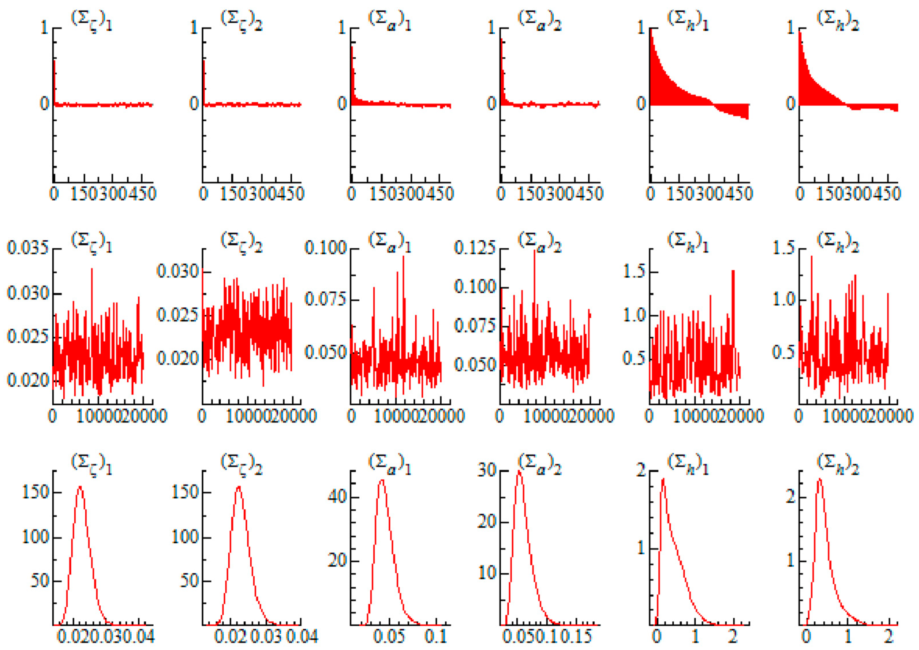
| Mean | St. Dev | 95%L | 95%U | Geweke | Inef. | |
|---|---|---|---|---|---|---|
| 0.0227 | 0.0026 | 0.0183 | 0.0286 | 0.2150 | 3.9600 | |
| 0.0230 | 0.0027 | 0.0185 | 0.0290 | 0.3410 | 2.8200 | |
| 0.0453 | 0.0092 | 0.0310 | 0.0667 | 0.0230 | 8.3900 | |
| 0.0444 | 0.0086 | 0.0309 | 0.0641 | 0.0930 | 11.4500 | |
| 0.5335 | 0.3378 | 0.0752 | 1.2870 | 0.1080 | 125.3200 | |
| 0.3431 | 0.1722 | 0.1036 | 0.7669 | 0.6420 | 63.5400 |
| Mean | St. Dev | 95%L | 95%U | Geweke | Inef. | |
|---|---|---|---|---|---|---|
| 0.0228 | 0.0027 | 0.0184 | 0.0287 | 0.3550 | 4.5000 | |
| 0.0230 | 0.0027 | 0.0185 | 0.0289 | 0.5260 | 3.2000 | |
| 0.0445 | 0.0088 | 0.0308 | 0.0650 | 0.5580 | 10.3100 | |
| 0.0505 | 0.0108 | 0.0336 | 0.0754 | 0.4100 | 12.0700 | |
| 0.4923 | 0.3177 | 0.0858 | 1.1984 | 0.2590 | 103.9000 | |
| 0.4434 | 0.2130 | 0.1547 | 0.9810 | 0.2930 | 78.8900 |
| Mean | St. Dev | 95%L | 95%U | Geweke | Inef. | |
|---|---|---|---|---|---|---|
| 0.0228 | 0.0026 | 0.0183 | 0.0284 | 0.4130 | 2.9400 | |
| 0.0230 | 0.0027 | 0.0184 | 0.0291 | 0.3460 | 4.6700 | |
| 0.0462 | 0.0096 | 0.0316 | 0.0686 | 0.1720 | 19.6300 | |
| 0.0599 | 0.0157 | 0.0373 | 0.0971 | 0.2420 | 14.9100 | |
| 0.4279 | 0.2924 | 0.0743 | 1.1305 | 0.5250 | 138.0900 | |
| 0.4495 | 0.2496 | 0.1159 | 1.1173 | 0.9050 | 107.8300 |
© 2018 by the authors. Licensee MDPI, Basel, Switzerland. This article is an open access article distributed under the terms and conditions of the Creative Commons Attribution (CC BY) license (http://creativecommons.org/licenses/by/4.0/).
Share and Cite
He, X.; Cai, X.-J.; Hamori, S. Bank Credit and Housing Prices in China: Evidence from a TVP-VAR Model with Stochastic Volatility. J. Risk Financial Manag. 2018, 11, 90. https://doi.org/10.3390/jrfm11040090
He X, Cai X-J, Hamori S. Bank Credit and Housing Prices in China: Evidence from a TVP-VAR Model with Stochastic Volatility. Journal of Risk and Financial Management. 2018; 11(4):90. https://doi.org/10.3390/jrfm11040090
Chicago/Turabian StyleHe, Xie, Xiao-Jing Cai, and Shigeyuki Hamori. 2018. "Bank Credit and Housing Prices in China: Evidence from a TVP-VAR Model with Stochastic Volatility" Journal of Risk and Financial Management 11, no. 4: 90. https://doi.org/10.3390/jrfm11040090
APA StyleHe, X., Cai, X.-J., & Hamori, S. (2018). Bank Credit and Housing Prices in China: Evidence from a TVP-VAR Model with Stochastic Volatility. Journal of Risk and Financial Management, 11(4), 90. https://doi.org/10.3390/jrfm11040090