Mean-Variance Portfolio Selection in a Jump-Diffusion Financial Market with Common Shock Dependence


1
School of Mathematical Sciences, Nankai University, Tianjin 300071, China
2
School of Mathematics, Sun Yat-sen University, Guangzhou 510275, China
*
Author to whom correspondence should be addressed.
J. Risk Financial Manag. 2018, 11(2), 25; https://doi.org/10.3390/jrfm11020025
Submission received: 3 April 2018
/
Revised: 9 May 2018
/
Accepted: 14 May 2018
/
Published: 16 May 2018
(This article belongs to the Section Mathematics and Finance)
Abstract
:This paper considers the optimal investment problem in a financial market with one risk-free asset and one jump-diffusion risky asset. It is assumed that the insurance risk process is driven by a compound Poisson process and the two jump number processes are correlated by a common shock. A general mean-variance optimization problem is investigated, that is, besides the objective of terminal condition, the quadratic optimization functional includes also a running penalizing cost, which represents the deviations of the insurer’s wealth from a desired profit-solvency goal. By solving the Hamilton-Jacobi-Bellman (HJB) equation, we derive the closed-form expressions for the value function, as well as the optimal strategy. Moreover, under suitable assumption on model parameters, our problem reduces to the classical mean-variance portfolio selection problem and the efficient frontier is obtained.
1. Introduction
In the past two decades, the problems of optimal investment and optimal reinsurance have gained rich attention in actuarial and financial literature. One of the insurer’s objectives is to maximize the expected terminal wealth or minimize the ruin probability. See, for example, Browne (1995), Schmidli (2002) and Yang and Zhang (2005). The other impressive objective is to maximize the expected present value of total dividends. We refer the readers to Asmussen et al. (2000), Azcue and Muler (2005) and Bai and Guo (2010).
As is known, mean-variance portfolio selection problem is to explore a satisfactory wealth allocation for the sake of achieving the optimal trade-off between the expected investment return and its risk, which is measured by variance. It is a significant criterion to use mean-variance measuring the risk in financial theory, which was first proposed by Markowitz (1952). From then on, more and more researchers have been devoted to this field. See, for example, Lim (2004), Merton (1972) and Zhou and Li (2000). Subsequently, Bäuerle (2005) first put forward that the criterion of mean-variance may be attractive in insurance applications and then investigated optimal reinsurance strategy when the insurance risk process is described by a classical compound Poisson process. Afterwards, Bai and Zhang (2008) and Bi and Guo (2013) considered the optimal mean-variance reinsurance-investment problem under constrained controls. However, the aforementioned literature solving the underlying investment or reinsurance problems mainly concentrated on the stochastic control theory (for more details readers may consult Fleming and Soner (2006), Yong and Zhou (1999) and references therein).
Although many insightful results for various optimal control problems are available in the actuarial literature, most of them are derived under the assumption of independent risks. In reality, the risks of different types are often dependent in some way, which can be frequently seen in the literature of classical risk theory, for example, Cojocaru (2017), Cossette and Marceau (2000) and so on. In the theory of stochastic optimal control, there are three cases related to the common shock model. One typical case is the so-called common shock risk model, in which two or more claims with different classes are correlated due to a common shock. Based on two different kinds of dependent insurance businesses, Bai et al. (2013) investigated the optimal excess-of-loss reinsurance strategy under the criterion of minimizing the ruin probability for the controlled diffusion process. Liang and Yuen (2016) studied the optimal reinsurance problem to maximize the expected exponential utility under the principle of variance premium. Ming et al. (2016) considered the optimal reinsurance problem for a mean-variance optimizer. Bi et al. (2016) derived the optimal investment-reinsurance strategies with and without bankruptcy prohibition under the criterion of mean-variance. For more than two correlated claim number processes, Yuen et al. (2015) explored optimal reinsurance strategy for the problem of exponential utility maximization. The second frequently-used model describes that financial market and insurance risk are dependent with each other, i.e., the risky asset and insurance claims are correlated by a common shock. Based on this kind of common shock, Liang et al. (2016, 2017) studied the optimal reinsurance-investment problems under the mean-variance and exponential utility criterion, respectively. The third classical model expresses that the price processes of two or more risky assets in financial markets are correlated through a common shock. For example, Zhang and Liang (2017) investigated the optimal investment strategy under the criterion of maximizing the mean-variance utility with state dependent risk aversion.
Additionally, this paper considers a running penalizing cost, with a deterministic goal process to be achieved for the insurer and extends the existing results of the classical mean-variance problem. As is known, this results in the optimization problem with wealth-path dependence (see Bouchard and Pham (2004)). Moreover, we incorporate dependent risks between the stock price and claims into the model, which makes our modeling framework more realistic. Then we consider a general mean-variance problem, that is, besides the objective of expected terminal condition, the quadratic optimization functional includes also a running penalizing cost deviating from a deterministic target. Furthermore, our problem reduces to the classical mean-variance problem under suitable assumption on model parameters. It should be noted that our paper is different from Delong (2005) and Delong and Gerrard (2007). In fact, Delong (2005) considered a quadratic optimization problem only with a running penalizing cost deviating from a deterministic target but without considering the expected terminal objective. Meanwhile, Delong and Gerrard (2007) considered a general mean-variance problem, however, with independent risks between the risky asset and claims.
This paper is organized as follows. Section 2 presents the insurance risk process and two assets in financial market and then formulates a general mean-variance optimization problem. In Section 3, we derive closed-form expressions for both the value function and the optimal strategy via the HJB equation method . In Section 4, the efficient strategy and efficient frontier are obtained for the special case . Section 5 illustrates the impact of dependence and economic parameters on the efficient frontier. Finally, Section 6 concludes the paper.
2. The Model
2.1. Some Necessary Notations
Let be a finite interval and be a complete probability space. Denote by the set of all real numbers. Let be a standard Brownian motion, , and be three homogeneous Poisson processes with intensity parameters , and , respectively. Throughout this paper, we assume that , , and are mutually independent. We define as the natural filtration generated by , , and satisfying the usual conditions.
2.2. The Insurance Risk Process
The risk process of the insurer is modeled by
where c is a constant premium rate, represents the number of claims occurring in the time interval , and is a sequence of positive-valued i.i.d random variables, which represents the size of the ith claim. Let X be a generic random variable which has the same distribution as . Denote and . Here, we assume , and are mutually independent, and the premium is paid in accordance with the expected premium principle, i.e.,
where and is the insurer’s safety loading.
2.3. Description of Financial Market
We consider a financial market consisting of two assets. One is a risk-free asset, such as bond or bank account, the other one is risky asset, such as stock or mutual fund. Specially, the price of the risk-free asset is given by
where represents the risk-free interest rate.
The price of the risky asset is driven by the following jump-diffusion process
where implies that the expected return rate of the stock price is larger than the risk-free interest rate, and is the coefficient of volatility, which reflects the gradual fluctuation of stock price due to the change of economic environment. Here, we assume that are a sequence of i.i.d random variables with values in and have the same distribution as a generic random variable Y. Denote and . This jump component characterizes the sudden fluctuation of stock price due to the appearance of some unpredictable information which may have influence on the stock price. It is worth noting that the assumption is essential, since it guarantees that the stock prices are always positive. Clearly, the dependence between risky asset and aggregate claim is correlated by a common shock described by Poisson process . Following Protter (2004, Chapter V), Equation (2) admits a unique solution.
2.4. Problem Formulation
Suppose that the insurer can invest all its wealth into the financial market. Denote by the total money invested into the stock at time t. In this paper, short-selling is allowed, i.e., is real-valued. Incorporating strategy into (1) and denoting by the controlled wealth process, we have
Definition 1.
A strategy is said to be admissible, if is -predictable and satisfies . Denote by Π the set of all admissible strategies.
Remark 1.
For any admissible strategy , it is not difficult to prove that Equation (3) admits a unique solution on .
We suppose that besides the objective of terminal condition, the quadratic optimization functional includes also a running penalizing cost representing deviations of the wealth process from a desired goal process . Then the optimal quadratic investment problem with a running penalizing cost can be established as the following general mean-variance optimization problem:
where attaches a weight to the terminal cost. Here we assume that is Lipschitz continuous with respect to t which could denote a profit accumulated until time t. For instance, , where may represent the desired expected return rate of the wealth. It is easy to see that (4) reduces to the following classical mean-variance problem when is deterministic and :
Remark 2.
It should be noted that adding the running penalizing cost into the optimization problem is reasonable since the optimal strategy in this case should guarantee that the controlled wealth process is not far away from the target process during the whole term of the contract.
3. The Closed-Form Solution to HJB Equation
This section focuses on solving the general quadratic optimization problem (4) stated in Section 2. Note that problem (4) is a convex optimization problem and can be tackled by introducing a Lagrange multiplier. Hence, we first solve the inner stochastic control problem given a fixed Lagrange multiplier
and then determine the optimal such that the following equality holds
where is the optimal strategy of (6).
We now give the definition of the associated value function for problem (6)
where represents the conditional expectation under given that . According to Fleming and Soner (2006), the corresponding HJB equation can be formulated as
with the boundary condition
where the generator is given by
Next, we propose a specific discussion on deriving a continuously differentiable solution to HJB Equation (7).
Theorem 1.
A continuously differentiable solution to HJB Equation (7) is given by
and the optimal investment strategy is expressed as
where , , have the following closed-form expressions
with , , and , , determined by (13)–(15) and (17)–(19), respectively.
Proof.
Suppose is a solution to Equation (7) which can be expressed as
According to the terminal condition (8), we have
Inserting (11) back into Equation (7) yields
If , differentiating (12) with respect to results in
It is obvious that (12) attains its minimum at
where , and are given by
Substituting back into (12) yields
By separating the variables with respect to x we obtain the following three ODEs:
where , and for are given by
As a result, the solutions , and of (16) are expressed by (10). Specially, it is not difficult to verify that , which implies that the infimum in (7) can be obtained. We complete the proof. □
Denote by the set of all continuous functions defined on such that its first-order and second-order partial derivatives , , are real-valued continuous. Using the standard methods of Fleming and Soner (2006), we present the following classical verification theorem.
Theorem 2.
If satisfies the following inequality
with
Then
Furthermore, if there exists an admissible strategy such that
then , and is the optimal investment strategy.
Remark 3.
Following the verification theorem, it is easy to obtain that presented by Theorem 1 is identical to and given by (9) is the optimal investment strategy. For the detailed proof of Theorem 2, readers may consult the Appendix in Delong and Gerrard (2007). Here we omit it.
Next, we devote to exploring the optimal value of Lagrange multiplier . Substituting back into the Equation (3) yields
Rewrite the above Itô differential in the integral form
Denote
Taking expectation on both sides of (20) under the condition , and then applying Fubini’s theorem to the right-hand side yield
Clearly, the function defined in (21) is continuously differentiable with respect to t. Hence, the integral form in (21) can be transformed into the following ODE:
which can be easily solved and leads to
Therefore, it suffices to determine the optimal value of which can make the constraint hold. After some algebraic calculations we deduce the value of the Lagrange multiplier
where
and
Next, we conclude the above results with the following theorem.
Theorem 3.
Let , and be given by (13)–(15). Then the optimal investment strategy for the constrained quadratic optimization problem (4) is given by
and the quadratic minimum cost is
where the functions , , and the Lagrange multiplier β are presented by (10) and (22), respectively.
4. Efficient Strategy and Efficient Frontier
This section concentrates on deriving the efficient strategy and efficient frontier for the classical mean-variance problem (5). Note that the efficient strategy can be easily obtained by setting in Theorem 3:
As is mentioned in Bielecki et al. (2005), the efficient frontier is the subset of the variance minimizing frontier, which can be obtained from the optimal value function under the condition of . After some algebraic calculations, it is not difficult to derive the Lagrange multiplier which has the following form
and the variance minimizing frontier equals
where
Remark 4.
Similar to Delong and Gerrard (2007), we have . Note that when , it is obvious that there exists no “risk-free asset", i.e., there exists no investment strategy such that the risk is zero. This is reasonable since implies larger intensities of the claims forthcoming. Thus, even though we invest all our wealth into the risk-free asset, that is, choosing the expected return target , we are still exposed to risks with a strictly positive probability due to the large amount of claims. On the other hand, this is in accordance with the results of classical mean-variance investment-reinsurance problem, see Liang et al. (2016), in which case there exists real “risk-free asset" indeed. The comparisons can also be seen in Remark 5 in Section 5.
Now, let us end the results by introducing the following straightforward lemma.
Lemma 1.
The variance minimizing frontier (27) is strictly decreasing for and strictly increasing for , where
and is expressed as (18). Moreover, the efficient frontier is , where .
5. Sensitive Analysis
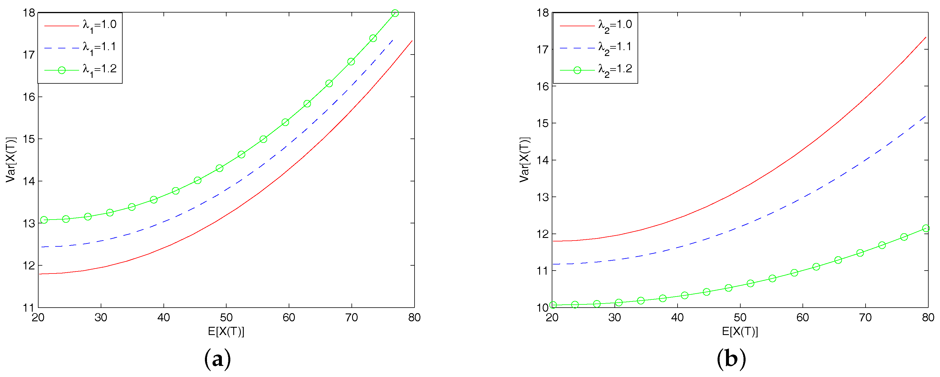
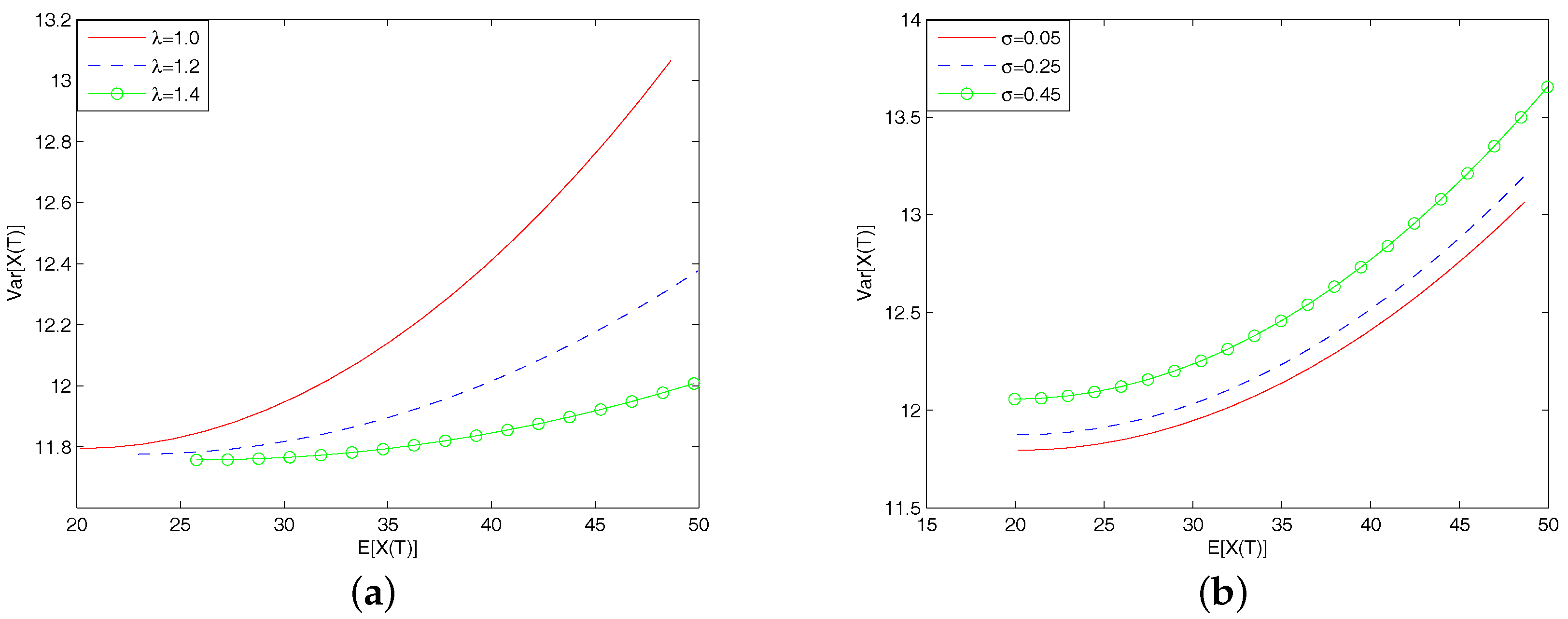
This section presents several numerical examples to illustrate the impact of different parameters on the efficient frontier derived in the previous section. Set , , , , , , , , ,
(i) Figure 1 investigates the impact of parameters and on the efficient frontier. In Figure 1a, we assume that the value of varies and the other parameters are fixed. It shows that under the same , increases with . This is a natural consequence since under the same expected terminal wealth, the bigger , the more frequency the claims arrive, which results in more risks the insurer undertakes. In Figure 1b, we assume that the value of varies and the other parameters are fixed. Different from Figure 1a, the bigger , the more frequency the stock price jumps upwards, which leads to bigger expected terminal wealth under the same .
(ii) Figure 2 illustrates the impact of common shock intensity and the volatility coefficient on the efficient frontier. In Figure 2a, we assume that the common shock intensity varies and the other parameters are fixed. It shows that under the same , decreases with . As increases, the insurer will receives more premium and then he would be more likely to invest his wealth into the risk-free asset rather than risky asset to hedge the forthcoming claims. Therefore, the insurer prefers to possessing less risky asset to achieve the same expected terminal wealth, which leads to the decreasing of . In Figure 2b, we assume that the value of varies and the other parameters are fixed. It shows that under the same , increases with . This is obvious since influences the volatility rate of stock price. As increases, the volatility rate of stock price increases and the instantaneous growth rate remains unchanged. As a result, the insurer will undertake more risks to reach the same expected terminal wealth.
Remark 5.
From the four cases of numerical analysis presented in the above, we can conclude:
(i) Under the assumption of , stays always above zero whatever takes, which implies that the risk is always positive whatever the strategy we choose. In other words, there exists no investment strategy such that the risk is zero or there exists no “risk-free asset".
(ii) Note that this is different from the results in Liang et al. (2016, Section 5), where can always reach zero when takes on appropriate value. That is, the risk is zero if the insurer invests all his wealth into the risk-free asset and cedes all the claims to the reinsurer. In other words, there exists a special strategy such that the risk is zero or there exists “risk-free asset" indeed.
6. Conclusions
This paper considers a general mean-variance investment problem, that is, besides the objective of expected terminal condition, the quadratic optimization functional includes also a running penalizing cost, which describes the deviations of insurer’s wealth from a desired profit-solvency goal. Suppose that the stock price and the insurance claims are dependent via a common shock. Applying the theory of HJB equation, we derive explicit formula for the optimal investment strategy. Moreover, our problem reduces to the classical mean-variance problem, which is in accordance with the results in Liang et al. (2016).
Author Contributions
The two authors contribute equally to this article.
Acknowledgments
The authors would like to thank two anonymous reviewers for their careful reading and helpful comments on an earlier version of this paper, which leads to a considerable improvement of the presentation of the work. This work was supported by the National Natural Science Foundation of China (Grant No. 11571189) and the China Postdoctoral Science Foundation (Grant No. 2017M612787).
Conflicts of Interest
The authors declare no conflict of interest.
References
- Asmussen, Søren, Bjarne Højgaard, and Michael Taksar. 2000. Optimal risk control and dividend distribution policies. Example of excess-of loss reinsurance for an insurance corporation. Finance and Stochastics 4: 299–324. [Google Scholar] [CrossRef]
- Azcue, Pablo, and Nora Muler. 2005. Optimal reinsurance and dividend distribution policies in the Cramér-lundberg model. Mathematical Finance 15: 261–308. [Google Scholar] [CrossRef]
- Bäuerle, Nicole. 2005. Benchmark and mean-variance problems for insurers. Mathematical Methods of Operations Research 62: 159–65. [Google Scholar] [CrossRef]
- Bai, Lihua, and Huayue Zhang. 2008. Dynamic mean-variance problem with constranit risk control for the insurers. Mathematical Methods of Operations Research 68: 181–205. [Google Scholar] [CrossRef]
- Bai, Lihua, and Junyi Guo. 2010. Optimal dividend payments in the classical risk model when payments are subject to both transaction costs and taxes. Scandinavian Actuarial Journal 1: 36–55. [Google Scholar] [CrossRef]
- Bai, Lihua, Jun Cai, and Ming Zhou. 2013. Optimal reinsurance policies for an insurer with a bivariate reserve risk process in a dynamic setting. Insurance: Mathematics and Economics 53: 664–70. [Google Scholar] [CrossRef]
- Bi, Junna, and Junyi Guo. 2013. Optimal mean-variance problem with constrained controls in a jump-diffusion financial market for an insurer. Journal of Optimization Theory and Applications 157: 252–75. [Google Scholar] [CrossRef]
- Bi, Junna, Zhibin Liang, and Fangjun Xu. 2016. Optimal mean-variance investment and reinsurance problems for the risk model with common shock dependence. Insurance: Mathematics and Economics 70: 245–58. [Google Scholar] [CrossRef]
- Bielecki, T. R., H. Jin, S. R. Pliska, and X. Y. Zhou. 2005. Dynamic mean-variance with portfolio selection with bankruptcy prohibition. Mathematical Finance 15: 213–44. [Google Scholar] [CrossRef]
- Bouchard, Bruno, and Huyên Pham. 2004. Wealth-path dependent utility maximization in incomplete financial markets. Finance and Stochastics 8: 579–603. [Google Scholar] [CrossRef]
- Browne, Sid. 1995. Optimal investment policies for a firm with a random risk process: Exponentional utility and minimizing the probability of ruin. Mathematics of Operations Research 20: 937–58. [Google Scholar] [CrossRef]
- Cojocaru, Ionica. 2017. Ruin probabilities in multivariate risk models with periodic common shock. Scandinavian Actuarial Journal 2: 159–74. [Google Scholar] [CrossRef]
- Cossette, Hélene, and Etienne Marceau. 2000. The discrete-time risk model with correlated classes of business. Insurance: Mathematics and Economics 26: 133–49. [Google Scholar] [CrossRef]
- Delong, Łukasz. 2005. Optimal investment strategy for a non-life insurance company: Quadratic loss. Applications of Mathematics 32: 263–77. [Google Scholar] [CrossRef]
- Delong, Łukasz, and Russell Gerrard. 2007. Mean-variance portfolio selection for a non-life insurance company. Mathematical Methods of Operations Research 66: 339–67. [Google Scholar] [CrossRef]
- Fleming, Wendell H., and Halil Mete Soner. 2006. Controled Markov Processes and Viscosity Solutions. New York: Springer. [Google Scholar]
- Liang, Zhibin, and Kam Chuen Yuen. 2016. Optimal dynamic reinsurance with dependent risks: Variance premium principle. Scandinavian Actuarial Journal 1: 18–36. [Google Scholar] [CrossRef] [Green Version]
- Liang, Zhibin, Kam Chuen Yuen, and Caibin Zhang. 2017. Optimal reinsurance and investment in a jump-diffusion financial market with common shock dependence. Journal of Applied Mathematics and Computing 56: 637–64. [Google Scholar] [CrossRef]
- Liang, Zhibin, Junna Bi, Kam Chuen Yuen, and Caibin Zhang. 2016. Optimal mean-variance reinsurance and investment in a jump-diffusion financial market with common shock dependence. Mathematical Methods of Operations Research 84: 155–81. [Google Scholar] [CrossRef]
- Lim, Andrew EB. 2004. Quadratic hedging and mean-variance portfolio selection with random parameters in an incomplete market. Mathematics of Operations Research 29: 132–61. [Google Scholar] [CrossRef]
- Markowitz, Harry. 1952. Portfolio selection. Journal of Finance 7: 77–91. [Google Scholar]
- Merton, Robert C. 1972. An analytical derivation of the efficient portfolio frontier. Journal of Financial and Quatative Analysis 7: 1851–72. [Google Scholar] [CrossRef]
- Ming, Zhiqin, Zhibin Liang, and Caibin Zhang. 2016. Optimal mean-variance reinsurance with common shock dependence. Anziam Journal 58: 162–81. [Google Scholar] [CrossRef]
- Protter, Philip E. 2004. Stochastic Integration and Differential Equations, 2nd ed. Berlin: Springer. [Google Scholar]
- Schmidli, Hanspeter. 2002. On minimizing the ruin probability by investment and reinsurance. Annals of Applied Probability 12: 890–907. [Google Scholar] [CrossRef]
- Yang, Hailiang, and Lihong Zhang. 2005. Optimal investment for an insurer with jump-diffusion risk process. Insurance: Mathematics and Economics 37: 615–34. [Google Scholar] [CrossRef]
- Yong, Jiongmin, and Xun Yu Zhou. 1999. Stochastic Controls: Hamilton Systems and HJB Equations. New York: Springer. [Google Scholar]
- Yuen, Kam Chuen, Zhibin Liang, and Ming Zhou. 2015. Optimal proportional reinsurance with common shock dependence. Insurance: Mathematics and Economics 64: 1–13. [Google Scholar] [CrossRef] [Green Version]
- Zhang, Caibin, and Zhibin Liang. 2017. Portfolio optimization for jump-diffusion risky asset with common shock dependence and state dependent risk aversion. Optimal Control Applications and Methods 38: 229–46. [Google Scholar] [CrossRef]
- Zhou, Xun Yu, and Duan Li. 2000. Continuous-time mean-variance portfolio selection: A stochastic LQ framework. Applied Mathematics and Optimization 42: 19–33. [Google Scholar] [CrossRef]
Figure 1.
Impact of parameters and on the efficient frontier. (a) Impact of on the efficient frontier; (b) Impact of on the efficient frontier.
Figure 1.
Impact of parameters and on the efficient frontier. (a) Impact of on the efficient frontier; (b) Impact of on the efficient frontier.

Figure 2.
Impact of parameters and on the efficient frontier. (a) Impact of on the efficient frontier; (b) Impact of on the efficient frontier.
Figure 2.
Impact of parameters and on the efficient frontier. (a) Impact of on the efficient frontier; (b) Impact of on the efficient frontier.

© 2018 by the authors. Licensee MDPI, Basel, Switzerland. This article is an open access article distributed under the terms and conditions of the Creative Commons Attribution (CC BY) license (http://creativecommons.org/licenses/by/4.0/).
Share and Cite
MDPI and ACS Style
Tian, Y.; Sun, Z. Mean-Variance Portfolio Selection in a Jump-Diffusion Financial Market with Common Shock Dependence. J. Risk Financial Manag. 2018, 11, 25. https://doi.org/10.3390/jrfm11020025
AMA Style
Tian Y, Sun Z. Mean-Variance Portfolio Selection in a Jump-Diffusion Financial Market with Common Shock Dependence. Journal of Risk and Financial Management. 2018; 11(2):25. https://doi.org/10.3390/jrfm11020025
Chicago/Turabian StyleTian, Yingxu, and Zhongyang Sun. 2018. "Mean-Variance Portfolio Selection in a Jump-Diffusion Financial Market with Common Shock Dependence" Journal of Risk and Financial Management 11, no. 2: 25. https://doi.org/10.3390/jrfm11020025