Testing for Causality-In-Mean and Variance between the UK Housing and Stock Markets

Shinsei Bank, Limited, 4-3, Nihonbashi-muromachi 2-chome, Chuo-ku, Tokyo 103-8303, Japan
J. Risk Financial Manag. 2018, 11(2), 21; https://doi.org/10.3390/jrfm11020021
Submission received: 24 March 2018
/
Revised: 6 April 2018
/
Accepted: 6 April 2018
/
Published: 26 April 2018
(This article belongs to the Special Issue Empirical Finance)
Abstract
:This paper employs the two-step procedure to analyze the causality-in-mean and causality-in-variance between the housing and stock markets of the UK. The empirical findings make two key contributions. First, although previous studies have indicated a one-way causal relation from the housing market to the stock market in the UK, this paper discovered a two-way causal relation between them. Second, a causality-in-variance as well as a causality-in-mean was detected from the housing market to the stock market.
JEL Classification:
C22; E44; G11
1. Introduction
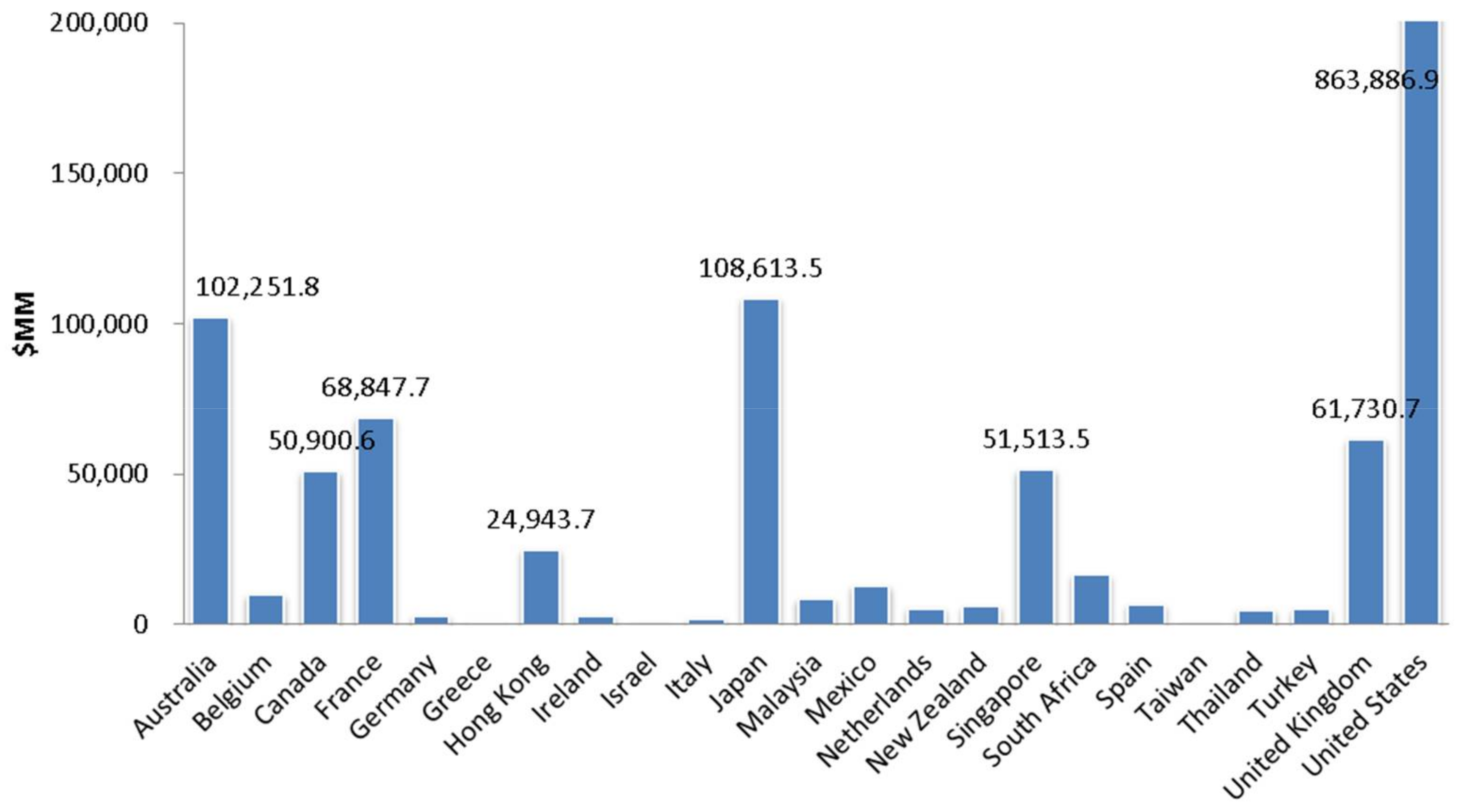
Although major financial institutions experienced the subprime mortgage crisis and Lehman Brothers went out of business, the market for real estate has grown steadily in the last decade. As indicated in Figure 1, the UK is one of the largest markets in the world, followed by the US, Japan, Australia, and France. In addition, since the UK decided to withdraw from the European Union (“Brexit”), based on a referendum conducted on 23 June 2016, market participants and macroeconomic policymakers have focused more on its impact on the UK real estate market. Therefore, examining the relation between the UK real estate and other financial markets is useful for both practitioners and academic researchers. Many previous empirical studies have explored the relation between the real estate and stock markets. Regarding this relation, we need to understand the following two effects. First, researchers who support the “wealth effect” claim that households benefiting from unanticipated gains in stock prices tend to increase housing demand. Second, researchers who support the “credit price effect” claim that an increase in real estate prices can stimulate economic activity and the future profitability of companies by raising the value of collateral and reducing the cost of borrowing for both companies and households. Thus, identifying the direction of causality between the real estate and stock markets as well as the number of lags is essential.
As mentioned above, many previous empirical studies have analyzed the relation between the real estate and stock markets (e.g., Gyourko and Keim (1992); Ibbotson and Siegel (1984); Ibrahim (2010); Kapopoulos and Siokis (2005); Lin and Fuerst (2014); Liow (2006); Liow (2012); Liow and Yang (2005); Louis and Sun (2013); Okunev and Wilson (1997); Okunev et al. (2000); Quan and Titman (1999); Su (2011); and Tsai et al. (2012)). To the best of our knowledge, no studies have analyzed the causality-in-variance between the real estate and stock markets. As indicated by Ross (1989), volatility provides useful data on the flow of information. For institutional investors such as banks, life insurance companies, hedge funds, and pension funds, deeper knowledge of spillover mechanisms for volatility can be useful for diversifying investments and hedge risk.
Table 1 summarizes the previous studies. Academic research on the relation between the real estate and stock markets has been undertaken since the 1980s. In this research, almost all studies have focused on the cointegration relation between the two markets. In recent years, not only a linear cointegration method but also a nonlinear cointegration method has been undertaken (e.g., Liow and Yang (2005); Okunev et al. (2000); Su (2011); and Tsai et al. (2012)). Using data from four major Asian countries (Japan, Hong Kong, Singapore, and Malaysia), Liow and Yang (2005) analyzed the relation between the securitized real estate and stock markets. Moreover, they conducted a fractional cointegration analysis of two asset markets. Furthermore, they revealed that fractional cointegration exists between the securitized real estate and stock markets of Hong Kong and Singapore. Okunev et al. (2000) examined the dynamic relation between the US real estate and S&P 500 stock index from 1972 to 1998 by conducting both linear and nonlinear causality tests. While the linear test results generally indicate a unidirectional relation from the real estate market to the stock market, nonlinear causality tests indicate a strong unidirectional relation from the stock market to the real estate market. Su (2011) used a nonparametric rank test to empirically investigate the long-run nonlinear equilibrium relation within Western European countries. Nonlinear causality test results demonstrated that unidirectional causality from the real estate market to the stock market exists in the Germany, the Netherlands, and the UK. Unidirectional causality from the stock market to the real estate market was observed in Belgium and Italy, and feedback effects were discovered in France, Spain, and Switzerland. Tsai et al. (2012) used nonlinear models to analyze the long-term relation between the US housing and stock markets. Empirical results demonstrated that the wealth effect between the stock and housing markets is more significant when the stock price outperforms the housing price by an estimated threshold level.
This paper uses the cross-correlation function (CCF) approach developed by Cheung and Ng (1996) to examine the causal relation between the housing and stock markets in the UK. This empirical technique has been widely applied in the examination of stock, fixed income, and commodities markets, business cycles, and derivatives.1 While the test of Granger causality techniques examines the causality-in-mean, the CCF approach detects both the causality-in-mean and causality-in-variance.2 The CCF approach can detect the direction of causality as well as the number of leads/lags involved.3 Furthermore, it permits flexible specification of the innovation process and nondependence on normality.4
The remainder of this paper is organized as follows. The next section presents the CCF approach. In the following sections, we discuss the data, descriptive statistics, and results of the unit root tests and provide a description of the autoregressive-exponential generalized autoregressive conditional heteroskedasticity (AR-EGARCH) specification. Thereafter, we present the empirical results and discuss the findings. Finally, a summary and conclusion are presented in the closing section.
2. Empirical Techniques
Following Cheung and Ng (1996), suppose there are two stationary and ergodic time series, and . When , , and are three information sets defined by , , and , Y is said to cause X in the mean if
Similarly, X is said to cause Y in the mean if
Feedback effect in the mean occurs if Y causes X in the mean and X causes Y in the mean. On the other hand, Y is said to cause X in the variance if
where denotes the mean of conditioned on . Similarly, X is said to cause Y in the variance if
where denotes the mean of conditioned on . Feedback effect in the variance occurs if X causes Y in the variance and Y causes X in the variance.
We impose the following structure in Equation (1) through Equation (4) to detect causality-in-mean and causality-in-variance. Suppose and are written as
where and are two independent white noise processes with zero mean and unit variance.
For the causality-in-mean test, we have the standardized innovation as follows:
with and being the standardized residuals. Since these residuals are unobservable, we use their estimates. Next, using their estimates, we calculate the sample cross-correlation of the squared standardized residual series, , and the sample cross-correlation caluculated using the standardized residual series, , at time lag k.
The quantities and are used to detect causality-in-mean and causality-in-variance, respectively, using the CCF approach.
First, we can detect the null hypothesis that there is no causality-in-mean using the following CCF statistic:
If the CCF test statistic is below the critical value calculated using the standard normal distribution, then we cannot reject the null hypothesis.
Second, we can detect the null hypothesis that there is no causality-in-variance using the test statistic, which is given by
If the CCF test statistic is below the critical value calculated using the standard normal distribution, then we cannot reject the null hypothesis.
The CCF approach is divided into two steps. First, we estimate univariate time-series models that consider the time variant conditional means and conditional variances. In this paper, we adopt the AR-EGARCH formulation.5 Second, from the estimated AR-EGARCH model, we calculate the standardized residuals of estimated model and calculate the series of standardized squared residuals by conditional variances. As mentioned above, we use the CCF of these standardized residuals to test the null hypotheses of no causality-in-mean and no causality-in-variance.
3. Data, Descriptive Statistics, and Results of an Augmented Dickey–Fuller Test
We employ monthly data on the UK housing and stock markets from January 1991 to August 2016. This sample period was chosen based on the availability of data obtained from The Nationwide Building Society.6
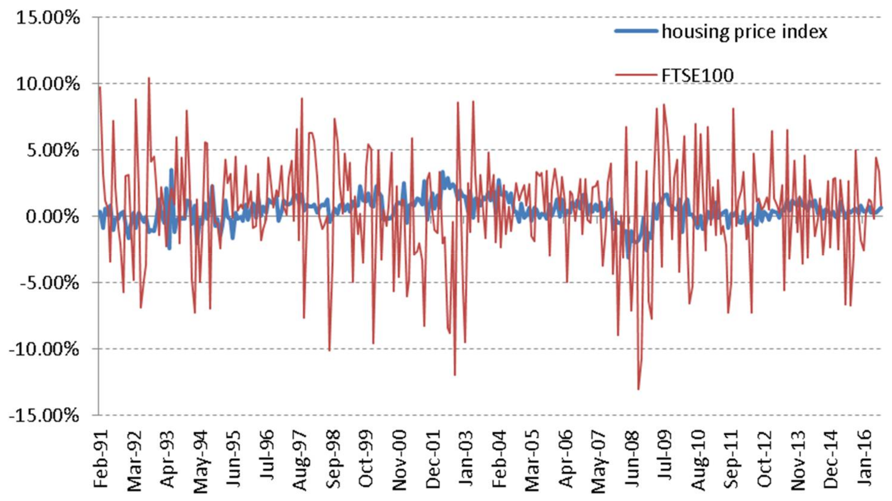
Table 2 presents the descriptive statistics for the monthly change rate in stock and housing prices. As indicated in Figure 2, the volatility of the stock market is higher than that of the housing market. The measure for skewness and kurtosis, Jarque–Bera statistics, are used to detect whether the housing and the stock monthly change rates are normally distributed.7 The Jarque–Bera statistics reject normality at a 10% significance level in both variables.
Table 3 indicates the results of the Augmented Dickey–Fuller test. The results reveal that, while the null hypothesis that the variables have a unit root is accepted in both variables in the level, the null hypothesis is rejected at the first difference.
4. Estimation of an AR-EGARCH Model
The first step of the CCF approach is to model the monthly change rates in the housing and stock prices. We estimate the AR(k)-EGARCH(p,q) model as follows:
where . Note that the left-hand side of Equation (13) is the log of the conditional variance. Using the log form of the EGARCH(p,q) model, it is possible to guarantee the non-negativity constraints without imposing the constraints of the coefficients.8 By including the term , the EGARCH(p,q) model reflects the asymmetric effect of positive and negative shocks. If then is positive. The persistence of shocks to the conditional variance is given by .
Equation (11), which is the conditional mean, is formulated as an autoregressive model of order k. To determine the optimal lag length k for each variables, we use the Schwartz–Bayesian Information Criterion (SBIC).9 The SBIC is also applied in Equation (13) to determine the optimal lag length p and q.10
Table 4 presents the estimates for the AR(k)-EGARCH(p,q) model. Regarding the standard error, this paper accepts the robust standard error developed by Bollerslev and Wooldridge (1992). First, the EGARCH(1,1) model is chosen for both variables. While all parameters of the EGARCH model in the monthly change rate in the stock price are significant, all parameters excluding in the monthly change rate in the housing price are significant at the conventional significance levels.
Furthermore, Table 4 reports the estimates of the coefficient , which measures the degree of volatility persistence. We find that is significant at conventional significance levels, and the value of is close to 1. These estimates lead to the conclusion that the persistence in shocks to volatility is relatively large. Table 2 also indicates the diagnostics of the empirical results of the AR-EGARCH model. While is a test statistic for the null hypothesis that there is no autocorrelation up to order 24 for standardized residuals, is a test statistic for the null hypothesis that there is no autocorrelation up to order 24 for standardized residuals squared.11 These tables show that both statistics are statistically significant at 5% level for all cases. Thus, the null hypothesis that there is no autocorrelation up to order 24 for standardized residuals and the standardized residuals squared is accepted. These results empirically support the formulation of the AR-EGARCH model.
5. Testing for Causality-In-Variance
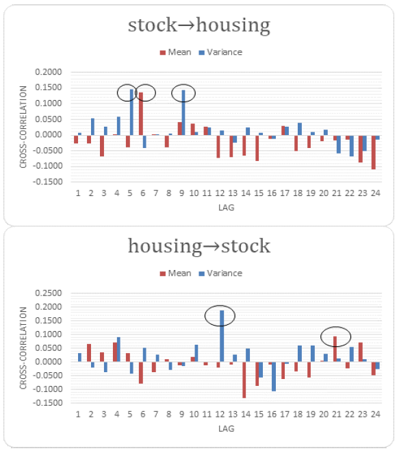
The second step is to detect causality-in-mean and causality-in-variance, using the calculated sample cross-correlations. Table 4 indicates the empirical results. Lags are measured in months, which range from 1 to 24. For example, in the case of “housing and stock (−k),” the significance of positive lags implies that the causal direction is from the stock market to the housing market.
Table 5 presents significance lags causality for both cases. First, in the case of “housing and stock (−k),” the causality-in-mean exists in lag 6 and the causality-in-variance exists in lags 5 and 9. Second, in the case of “housing and stock (+k),” the causality-in-mean exists in lags 21 and the causality-in-variance exists in lags 4 and 12. The above results provide two interesting findings. First, although Su (2011) indicated a one-way causal relation from the housing market to the stock market in the UK, this paper discovered a two-way causal relation between them. This supports the idea that both a wealth effect and a credit price effect exist between the housing and stock markets. Second, both causality-in-mean and causality-in-variance are detected from the housing market to the stock market. This finding has never been referred to in previous studies and it is useful for both practitioners and academic researchers.
6. Conclusions
This paper analyzes the causality-in-mean and causality-in-variance between the UK stock and housing markets using monthly data from January 1991 to August 2016. A CCF approach developed by Cheung and Ng (1996) and a causality-in-variance test applied to financial market prices are used as tests (Cheung and Ng 1996). The empirical findings make two key contributions. First, although Su (2011) showed a one-way causal relation from the housing market to the stock market in the UK, this paper discovered a two-way causal relation between them. Thus, both a wealth effect and a credit price effect exist between the housing and stock markets. This paper also detected a causality-in-mean and causality-in-variance from the housing market to the stock market. This point has never been referred to in previous studies and is useful for both practitioners and academic researchers.
Acknowledgments
We would like to thank three anonymous reviewers, whose valuable comments helped to improve an earlier version of this paper.
Conflicts of Interest
The author declares no conflict of interest.
References
- Alaganar, V. T., and Ramaprasad Bhar. 2003. An International Study of Causality-in-Variance: Interest Rate and Financial Sector Returns. Journal of Economics and Finance 27: 39–55. [Google Scholar] [CrossRef]
- Bhar, Ramaprasad, and Shigeyuki Hamori. 2005. Causality in Variance and the Type of Traders in Crude Oil Futures. Energy Economics 27: 527–39. [Google Scholar] [CrossRef]
- Bhar, Ramaprasad, and Shigeyuki Hamori. 2008. Information Content of Commodity Futures Prices for Monetary Policy. Economic Modelling 25: 274–83. [Google Scholar] [CrossRef]
- Bollerslev, Tim, and Jeffrey. M. Wooldridge. 1992. Quasi-Maximum Likelihood Estimation and Inference in Dynamic Models with Time Varying Covariances. Econometric Reviews 11: 143–72. [Google Scholar] [CrossRef]
- Chang, Chia-Lin, and Michael McAleer. 2017a. A simple test for causality in volatility. Econometrics 5: 15. [Google Scholar] [CrossRef]
- Chang, Chia-Lin, and Michael McAleer. 2017b. The correct regularity condition and interpretation of asymmetry in EGARCH. Economics Letters 161: 52–55. [Google Scholar] [CrossRef]
- Cheung, Yin-Wong, and Lilian K. Ng. 1996. A Causality-in-Variance Test and Its Applications to Financial Market Prices. Journal of Econometrics 72: 33–48. [Google Scholar] [CrossRef]
- Gyourko, Joseph, and Donald B. Keim. 1992. What Does the Stock Market Tell Us about Real Estate Returns? Journal of the American Real Estate Finance and Urban Economics Association 20: 457–86. [Google Scholar] [CrossRef]
- Hafner, Christian M., and Helmut Herwartz. 2008. Testing for Causality in Variance Using Multivariate GARCH Models. Annals of Economics and Statistics 89: 215–41. [Google Scholar] [CrossRef]
- Hamori, Shigeyuki. 2003. An Empirical Investigation of Stock Markets: The CCF Approach. Dordrecht: Kluwer Academic Publishers. [Google Scholar]
- Hong, Yongmiao. 2001. A Test for Volatility Spillover with Application to Exchange Rates. Journal of Econometrics 103: 183–224. [Google Scholar] [CrossRef]
- Hoshikawa, Takeshi. 2008. The Causal Relationships between Foreign Exchange Intervention and Exchange Rate. Applied Economics Letters 15: 519–22. [Google Scholar] [CrossRef]
- Ibbotson, Roger G., and Laurence B. Siegel. 1984. Real Estate Returns: A Comparison with Other Investments. Real Estate Economics 12: 219–42. [Google Scholar] [CrossRef]
- Ibrahim, Mansor H. 2010. House Price-Stock Price Relations in Thailand: An Empirical Analysis. International Journal of Housing Markets and Analysis 3: 69–82. [Google Scholar] [CrossRef]
- Jarque, Carlos M., and Anil K. Bera. 1987. Test for Normality of Observations and Regression Residuals. International Statistical Review 55: 163–72. [Google Scholar] [CrossRef]
- Kapopoulos, Panayotis, and Fotios Siokis. 2005. Stock and Real Estate Prices in Greece: Wealth versus Credit-Price Effect. Applied Economics Letters 12: 125–28. [Google Scholar] [CrossRef]
- Lin, Pin-te, and Franz Fuerst. 2014. The Integration of Direct Real Estate and Stock Markets in Asia. Applied Economics 46: 1323–34. [Google Scholar] [CrossRef]
- Liow, Kim Hiang, and Haishan Yang. 2005. Long-Term Co-Memories and Short-Run Adjustment: Securitized Real Estate and Stock Markets. The Journal of Real Estate Finance and Economics 31: 283–300. [Google Scholar] [CrossRef]
- Liow, Kim Hiang. 2006. Dynamic Relationship between Stock and Property Markets. Applied Financial Economics 16: 371–76. [Google Scholar] [CrossRef]
- Liow, Kim Hiang. 2012. Co-Movements and Correlations Across Asian Securitized Real Estate and Stock Markets. Real Estate Economics 40: 97–129. [Google Scholar] [CrossRef]
- Ljung, Greta M., and George E. P. Box. 1978. On a Measure of Lack of Fit in Time Series Models. Biometrika 66: 265–70. [Google Scholar] [CrossRef]
- Louis, Henock, and Amy X. Sun. 2013. Long-Term Growth in Housing Prices and Stock Returns. Real Estate Economics 41: 663–708. [Google Scholar] [CrossRef]
- McAleer, Michael, and Christian M. Hafner. 2014. A one line derivation of EGARCH. Econometrics 2: 92–97. [Google Scholar] [CrossRef] [Green Version]
- Miyazaki, Takashi, and Shigeyuki Hamori. 2013. Testing for causality between the gold return and stock market performance: Evidence for gold investment in case of emergency. Applied Financial Economics 23: 27–40. [Google Scholar] [CrossRef]
- Nakajima, Tadahiro, and Shigeyuki Hamori. 2012. Causality-in-Mean and Causality-in-Variance among Electricity Prices, Crude Oil Prices, and Yen-US Dollar Exchange Rates in Japan. Research in International Business and Finance 26: 371–86. [Google Scholar] [CrossRef]
- Nelson, Daniel B. 1991. Conditional Heteroskedasticity in Asset Returns: A New Approach. Econometrica 59: 347–70. [Google Scholar] [CrossRef]
- Okunev, John, and Patrick J. Wilson. 1997. Using Nonlinear Tests to Examine Integration between Real Estate and Stock Markets. Real Estate Economics 25: 487–503. [Google Scholar] [CrossRef]
- Okunev, John, Patrick Wilson, and Ralf Zurbruegg. 2000. The Causal Relationship between Real Estate and Stock Markets. Journal of Real Estate Finance and Economics 21: 251–61. [Google Scholar] [CrossRef]
- Quan, Daniel C., and Sheridan Titman. 1999. Do Real Estate Prices and Stock Prices Move Together? An International Analysis. Real Estate Economics 27: 183–207. [Google Scholar] [CrossRef]
- Ross, Stephen A. 1989. Information and Volatility: No-Arbitrage Martingale Approach to Timing and Resolution Irrelevancy. Journal of Finance 44: 1–17. [Google Scholar] [CrossRef]
- Su, Chi-Wei. 2011. Non-Linear Causality between the Stock and Real Estate Markets of Western European Countries: Evidence from Rank Tests. Economic Modelling 28: 845–51. [Google Scholar] [CrossRef]
- Schwarz, Gideon. 1978. Estimating the Dimension of a Model. Annals of Statistics 6: 461–64. [Google Scholar] [CrossRef]
- Tsai, I-Chun, Cheng-Feng Lee, and Ming-Chu Chiang. 2012. The Asymmetric Wealth Effect in the U.S. Housing and Stock Markets: Evidence from the Threshold Cointegration Model. Journal of Real Estate Finance and Economics 45: 1005–20. [Google Scholar] [CrossRef]
- Tamakoshi, Go, and Shigeyuki Hamori. 2014. Causality-in-variance and causality-in-mean between the Greek sovereignbond yields and Southern European banking sector equity returns. Journal of Economics and Finance 38: 627–42. [Google Scholar] [CrossRef]
- Toyoshima, Yuki, and Shigeyuki Hamori. 2012. Volatility Transmission of Swap Spreads among the United States, Japan, and the United Kingdom: A Cross-Correlation Function Approach. Applied Financial Economics 22: 849–62. [Google Scholar] [CrossRef]
| 1 | Some examples include studies by Hamori (2003), Alaganar and Bhar (2003), Bhar and Hamori (2005, 2008), Hoshikawa (2008), Nakajima and Hamori (2012), Miyazaki and Hamori (2013), Tamakoshi and Hamori (2014), and Toyoshima and Hamori (2012). |
| 2 | See Hafner and Herwartz (2008) and Chang and McAleer (2017a) for the causality-in-variance analysis using multivariate GARCH models. |
| 3 | |
| 4 | |
| 5 | |
| 6 | We obtained the data from the URL below: http://www.nationwide.co.U.K./about/house-price-index/download-data#tab:Downloaddata. |
| 7 | See Jarque and Bera (1987). |
| 8 | The EGARCH model suffers from a number of fundamental problems, including the lack of regularity conditions and hence the absence of any asymptotic properties. See McAleer and Hafner (2014) and Chang and McAleer (2017b) for details. |
| 9 | |
| 10 | We selected the final models from EGARCH(1,1), EGARCH(1,2), EGARCH(2,1), and EGARCH(2,2). |
| 11 | See Ljung and Box (1978). |
Figure 1.
Market capitalization of the S&P Global REIT (Real Estate Investment Trust) Index in August 2016. Data Source: S&P Capital IQ.
Figure 1.
Market capitalization of the S&P Global REIT (Real Estate Investment Trust) Index in August 2016. Data Source: S&P Capital IQ.

Figure 2.
Rates of change in the stock and housing indexes. Data Source: Nationwide Building Society, Yahoo Finance.
Figure 2.
Rates of change in the stock and housing indexes. Data Source: Nationwide Building Society, Yahoo Finance.


Table 1.
Summaries of previous studies.
| Authors | Empirical Technique | Country | Principal Results |
|---|---|---|---|
| Gyourko and Keim (1992) | Market regression model | the US | Lagged equity REIT and stock return are predictors of property index. |
| Ibbotson and Siegel (1984) | Correlation, Regression | the US | Low correlation between the real estate and stocks, bonds is found. |
| Ibrahim (2010) | VAR model, Granger causality tests | Thailand | Unidirectional causality from stock prices to house prices is found. |
| Kapopoulos and Siokis (2005) | VAR model, Granger causality tests | Greece | Unidirectional causality from stock prices to house prices is found. |
| Lin and Fuerst (2014) | Johansen, Gregory-Hansen ,Nonlinear cointegration tests | 9 Asian countries | Market segmentation is observed in China, Japan, Thailand, Malaysia, Indonesia and South Korea. |
| Liow (2006) | ARDL cointegration tests | Singapore | Contemporaneous long-term relationship between thestock market, residential and office property prices is found. |
| Liow (2012) | Asymmetric DCC model | 8 Asian countries | Conditional real estate-stock correlations are time varying and asymmetric in some cases. |
| Liow and Yang (2005) | FIVEC model, VEC model | 4 Asian countries | FIVECM improves the forecasting performance over conventional VECM models. |
| Louis and Sun (2013) | Fama–MacBeth procedure | the US | Firms’ long-term abnormal stock returns are negatively related to past growth in housing prices. |
| Okunev and Wilson (1997) | Cointegration tests | the US | Weak and nonlinear relationship between the stock and real estate markets is found. |
| Okunev et al. (2000) | Linear and nonlinear causality tests | the US | Strong uni-directional relationship from the stock market to the real estate market is found in nonlinear causality test. |
| Quan and Titman (1999) | Cross-sectional regression | 17 countries | Positive relation between real estate values and stock returns is found. |
| Su (2011) | TEC model, Non-parametric rank test | 8 Western European countries | Unidirectional causality from the real estate markets to the stock market is found in the Germany, Netherlands and the UK. |
| Tsai et al. (2012) | M-TAR cointegration model | the US | Threshold cointegration relationship between the housing market and the stock market is found. |
Table 2.
Descriptive Statistics: Rates of change in the stock and housing indexes.
| Statistics | Housing | Stock |
|---|---|---|
| Sample Size | 307 | 307 |
| Mean | 0.4421% | 0.4527% |
| Std. Dev. | 0.9544% | 4.0076% |
| Skewness | −0.2221 | −0.4557 |
| Kurtosis | 1.1434 | 0.5011 |
| Maximum | 3.4912% | 10.3952% |
| Minimum | −3.1084% | −13.0247% |
| Jarque-Bera | 19.2472 | 13.8362 |
| Probability | 0.0066% | 0.0990% |
Table 3.
Results of an augmented Dickey–Fuller test.
| Variable | Auxuliary Model | |||
|---|---|---|---|---|
| Const | Const & Trend | None | ||
| housing | Level | −0.2988 | −2.3811 | 1.5701 |
| First difference | −4.5065 *** | −4.5019 *** | −3.8047 *** | |
| stock | Level | −1.8598 | −2.2418 | 0.7945 |
| First difference | −17.3975 *** | −17.4146 *** | −17.2370 *** | |
Notes: *** indicates significance at 1%.
Table 4.
AR-EGARCH (autoregressive-exponential generalized autoregressive conditional heteroskedasticity) model.
Table 4.
AR-EGARCH (autoregressive-exponential generalized autoregressive conditional heteroskedasticity) model.
| Parameters | Housing | Stock | ||
|---|---|---|---|---|
| AR(3)-EGARCH(1,1) | AR(1)-EGARCH(1,1) | |||
| Estimate | SE | Estimate | SE | |
| a0 | 0.0021 *** | (0.0007) | 0.0088 *** | (0.0024) |
| a1 | 0.0321 | (0.061) | −0.0791 | (0.0602) |
| a2 | 0.4095 *** | (0.0518) | ||
| a3 | 0.2522 *** | (0.0582) | ||
| b0 | −0.0011 | (0.0007) | −0.007 * | (0.0037) |
| ω | −0.4465 * | (0.2485) | −1.3275 *** | (0.4386) |
| α1 | 0.2362 *** | (0.0818) | 0.3162 *** | (0.1148) |
| γ1 | −0.0074 | (0.0476) | −0.1191 * | (0.0614) |
| β1 | 0.9741 *** | (0.0224) | 0.8365 *** | (0.058) |
| Log Likelihood | 1074.4320 | 571.2161 | ||
| SBIC | −6.8994 | −3.6025 | ||
| Q(24) | 35.4320 | 11.6550 | ||
| P-value | 0.0620 | 0.9840 | ||
| Q2(24) | 0.0000 | 19.3240 | ||
| P-value | 0.0000 | 0.7350 | ||
Notes: ***, * indicate significance at 1% and 10%, respectively. and are the Ljung–Box (LB) statistics with 24 lags for the standardized residuals and their squares. In addition, we checked the lag of LB statistics from 1 to 24.
Table 5.
Cross-correlation for levels and squares of the standardized residuals.
| Lag k | Housing and Stock (−k) | Housing and Stock (+k) | ||
|---|---|---|---|---|
| Mean | Variance | Mean | Variance | |
| 1 | −0.0271 | 0.0067 | 0.0011 | 0.0320 |
| 2 | −0.0262 | 0.0549 | 0.0651 | −0.0196 |
| 3 | −0.0675 | 0.0259 | 0.0363 | −0.0358 |
| 4 | 0.0037 | 0.0589 | 0.0709 | 0.0920 * |
| 5 | −0.0390 | 0.1460 *** | 0.0322 | −0.0423 |
| 6 | 0.1366 *** | −0.0407 | −0.0797 | 0.0530 |
| 7 | 0.0016 | 0.0007 | −0.0380 | 0.0256 |
| 8 | −0.0386 | 0.0050 | 0.0105 | −0.0298 |
| 9 | 0.0410 | 0.1444 *** | −0.0114 | −0.0154 |
| 10 | 0.0375 | 0.0101 | 0.0179 | 0.0630 |
| 11 | 0.0269 | 0.0238 | −0.0132 | 0.0012 |
| 12 | −0.0728 | 0.0150 | −0.0204 | 0.1879 *** |
| 13 | −0.0695 | −0.0248 | −0.0084 | 0.0257 |
| 14 | −0.0648 | 0.0234 | −0.1309 | 0.0503 |
| 15 | −0.0835 | 0.0087 | −0.0859 | −0.0555 |
| 16 | −0.0120 | −0.0113 | −0.0087 | −0.1055 |
| 17 | 0.0301 | 0.0263 | −0.0620 | −0.0064 |
| 18 | −0.0497 | 0.0383 | −0.0341 | 0.0603 |
| 19 | −0.0406 | 0.0092 | −0.0573 | 0.0592 |
| 20 | −0.0200 | 0.0175 | 0.0051 | 0.0288 |
| 21 | −0.0161 | −0.0574 | 0.0944 ** | 0.0129 |
| 22 | −0.0141 | −0.0669 | −0.0235 | 0.0560 |
| 23 | −0.0868 | −0.0501 | 0.0720 | 0.0092 |
| 24 | −0.1098 | −0.0152 | −0.0469 | −0.0259 |
Notes: ***, **, * indicate significance at 1%, 5%, and 10%, respectively.
© 2018 by the author. Licensee MDPI, Basel, Switzerland. This article is an open access article distributed under the terms and conditions of the Creative Commons Attribution (CC BY) license (http://creativecommons.org/licenses/by/4.0/).
Share and Cite
MDPI and ACS Style
Toyoshima, Y. Testing for Causality-In-Mean and Variance between the UK Housing and Stock Markets. J. Risk Financial Manag. 2018, 11, 21. https://doi.org/10.3390/jrfm11020021
AMA Style
Toyoshima Y. Testing for Causality-In-Mean and Variance between the UK Housing and Stock Markets. Journal of Risk and Financial Management. 2018; 11(2):21. https://doi.org/10.3390/jrfm11020021
Chicago/Turabian StyleToyoshima, Yuki. 2018. "Testing for Causality-In-Mean and Variance between the UK Housing and Stock Markets" Journal of Risk and Financial Management 11, no. 2: 21. https://doi.org/10.3390/jrfm11020021