Article

Estimation of Cross-Lingual News Similarities Using Text-Mining Methods

1
Izumi lab, Department of System Innovation, Graduate School of Engineering, The University of Tokyo, Hongo 7-3-1, Bunkyo-ku, Tokyo 113-0033, Japan
2
Yahoo! Japan Research, Kioicho 1-3, Chiyoda-ku, Tokyo 102-8282, Japan
*
Authors to whom correspondence should be addressed.
J. Risk Financial Manag. 2018, 11(1), 8; https://doi.org/10.3390/jrfm11010008
Submission received: 31 December 2017 / Revised: 23 January 2018 / Accepted: 25 January 2018 / Published: 31 January 2018
(This article belongs to the Special Issue Empirical Finance)

Abstract

:
In this research, two estimation algorithms for extracting cross-lingual news pairs based on machine learning from financial news articles have been proposed. Every second, innumerable text data, including all kinds news, reports, messages, reviews, comments, and tweets are generated on the Internet, and these are written not only in English but also in other languages such as Chinese, Japanese, French, etc. By taking advantage of multi-lingual text resources provided by Thomson Reuters News, we developed two estimation algorithms for extracting cross-lingual news pairs from multilingual text resources. In our first method, we propose a novel structure that uses the word information and the machine learning method effectively in this task. Simultaneously, we developed a bidirectional Long Short-Term Memory (LSTM) based method to calculate cross-lingual semantic text similarity for long text and short text, respectively. Thus, when an important news article is published, users can read similar news articles that are written in their native language using our method.

1. Introduction

Text similarity, as its name suggests, refers to how similar a given text query is to others. We normally tend to consider texts based mainly on their semantic characteristics, that is, how close (i.e., similar) their meanings are. Here, the text could be in the form of character level, word level, sentence level, paragraph level, or even longer, document level. In this paper, we mainly discuss text that is in the form of sentences (i.e., short text) and documents (i.e., long text).
The objective of this research could be summarized in three key points. The fundamental objective is to develop algorithms for estimation of semantic similarity for the given two pieces of text written in different languages, applicable for both long text and short text, by taking advantage the untapped vast suppository of text resources from Thomson Reuters economics news reports. Secondly, as a practical application and a verification of our model, we are aiming at developing a cross-lingual recommendation system and test benchmark, which could provide several of the most-related (for example, 10 results) pieces of Japanese or English text when given an English (or Japanese) article. Thirdly, we excavate cross-lingual resources from the enormous database of Thomson Reuters News and build an effective cross-lingual system by taking advantage of this un-developed treasure.

2. Related Work and Theories

Regardless of the length of the text, most of the state-of-the-art methods have recently been implemented based on word embedding methods and thus we discuss this in detail in a separate section. To solve semantic text similarity problems, one of the most typical and inspiring methods is Siamese LSTM structure, which is considered as both a basis and a competitive baseline of this research.

2.1. Embedding Techniques for Words and Documents

Word embedding technique, also known as distributed word representation, is one of the most basic concepts and applications prevalent nowadays. Word embedding could be further extended to be performed on documents. The embedding techniques capture both the semantic and syntactic information and convert them into meaningful feature vectors which help to train accurate models for natural language processing (NLP) tasks (Tang et al. 2014).
Word embedding can be implemented for both monolingual and multilingual tasks. There are several successful papers working on the monolingual word embedding such as the continuous bag of words models and skip-gram models (Mikolov et al. 2013), monolingual document embedding such as doc2vec (Le and Mikolov 2014), cross-lingual word embedding (Zou et al. 2013), as well as cross-lingual document embedding models such as Bilingual Bag-of-Words without Word Alignments (BilBOWA) (Gouws et al. 2015). Through embedding model, each word, phrase or document would be converted into a fixed length vector representation, where the similarity between two words, phrases, or documents could be derived by calculating the cosine distance of their vector representations. Methods are distinctly different for the text data with different length when solving the text similarity problem (Le and Mikolov 2014). With respect to the length of the text, a textual similarity task could be further categorized into two sub-tasks. Prevalent methods for cross-lingual document (i.e., long text) similarity could be categorized into four aspects (Rupnik et al. 2016), Dictionary-based approaches (Kudo et al. 2004), Probabilistic topic model based approaches (Taghva et al. 2005), Matrix factorization based approaches (Lo et al. 2014), and Monolingual approaches.

2.2. Text Similarities Using Siamese LSTM

Neural network-based Siamese recurrent architectures have recently proved to be one of the most effective ways for learning semantic text similarity on the sentence level. Mueller, in his work, implements a Siamese recurrent structure called Manhattan LSTM (MaLSTM) (Mueller and Thyagarajan 2016), which is practically used as the estimation of relativeness (i.e., similarity) when given any two sentences in English. This structure uses Long Short-Term Memory (LSTM) (Hochreiter and Schmidhuber 1997) and has a state-of-the-art performance on both semantic relatednesses scoring task and entailment classification using the SICK database, one of the NLP challenges provided by SemEval (Agirre et al. 2016). This model could identify how two sentences are similar to each other by trying to “understand” their true meaning on a deeper aspect, like the sentence pairs “He is smart” and “A truly wise man” as the figure demonstrates. They have no common words with different lengths, but they are indeed highly relevant to each other in terms of their implications, which a human cannot recognize without more consideration and logical analysis, suggesting the difficulty of this challenge.
In our work, we developed a new recurrent structure inspired by MaLSTM, by modifying the Siamese (i.e., symmetric) LSTM modules to “unbalanced” ones, and adding a full-connect neural network layer following the output of LSTM modules, which is more flexible and effective than a text similarity task.

3. Methods for Extracting Cross-Lingual News Pairs

In this section, we will introduce all fundamental and necessary methods applied in our research. There are mainly three aspects to be elaborated, including methods we applied regarding the foundation of natural language processing, such as word embedding and TF-IDF. We explained two applied methods, one of which is the classical methods learning SVM (Support Vector Machine). The other one is the neural network method, LSTM(Long-Short Term Memory).

3.1. Distribution Representation

The most traditional and naive way to consider words as features is to treat words as discrete symbols or numbers. This results in a discrete representation of each word and hinders the establishment of relations among these features. In contrast, vector space models consider (embedded) words in a continuous vector space, in which words with similar meanings are separated by small distances. There are two main categories for continuous word embedding: count-based (such as latent semantic analysis) models and predictive-based methods (such as neural probabilistic language models). The count-based models focus on the co-occurrence of the considered word and its neighboring words, whereas the predictive-based models predict a word based on its neighbors using embedding vectors Baroni et al. (2014). In this research, we implement a predictive-based model that is known as word2vec; it is based on the skip-gram or continuous bag-of-words model Mikolov et al. (2013).
We train each word from the training text sequence w 1 , w 2 , w 3 , , w T to maximize the objective function
1 T t = 1 T c j c , j 0 log p ( w t + j | w t )
wherein c is the so-called “window size,” which determines how much context information is to be considered for each of the training words. More specifically, we define p ( w t + j | w t ) using a softmax function:
p ( w O | w I ) = exp ( v w O T v w I ) w = 1 W exp ( v w T v w I )
wherein W is the size of the vocabulary (i.e., the number of disparate words to be considered), and v is the vector representations for either the word w, the input word w I , or the output word w O .
However, the calculation of Equation (2) is impractical because the computational cost for calculating the gradient of log p ( w t + j | w t ) is proportional to W, which consists of as many as 10 5 to 10 7 terms. In practical terms, to train the model (i.e., optimize the cost function) in a more computationally efficient manner, we use Noise Contrastive Estimation for approximation during training, as described in Mikolov et al. (2013).
Finally, vector representations with fixed dimension (e.g., 200) can be extracted from the trained model. These word vectors have some outstanding attributes. Because we train our model for each word using its neighboring words, and words with similar meaning usually tend to have similar context, we can calculate the similarity among words using the cosine distance.

3.2. Term Frequency-Inversed Document Frequency (TF-IDF)

TF-IDF is one of the classical weighting models for words, which uses text representations. It is widely used in the natural language processing domain wherein it is commonly applied for weighting words or document features, such as in one-hot bag-of-words representation. The term frequency stands for the number of times a considered word occurs in a specific document, while the document frequency is the number of documents in the corpus that include the word. The inverse document frequency term for a specific word can be expressed as
i d f = log N 1 + d f
wherein N is the total number of documents in the corpus. Combining these two concepts, the TF-IDF weight is the product of the TF and the IDF. This scheme loses semantic information for words; thus, it usually cannot achieve satisfactory performance. However, it measures the weights and importance of each word inside documents and among other documents according to a reasonable definition. In this study, we apply TF-IDF to weight words during document embedding.

3.3. TF-IDF Weighting for Word Vectors

Although there are several ways to form vector representations for documents (i.e., document embedding), we have experimentally discovered that the most effective strategy is to use the TF-IDF weighted sum of the word vectors that are present in each document as features. First, we calculate two TF-IDF weighting models, namely TF-IDF j p and TF-IDF e n , for each word from English training documents and Japanese training documents. Second, for each Japanese document, the weighted sum document representation can be derived as
J i = m = 0 N i t i , m · w i , m
wherein N i refers to the number of words in this Japanese document (i.e., Japanese document i), and t i , m stands for the Japanese TF-IDF weight for the m-th word in document i with respect to the considered word. The final term w i , m is the word vector of the m-th word in document i, that is, the vector representation for this considered word.
We apply the same weighting scheme to the English documents. The vector representation for English document i can be expressed as
E i = m = 0 N i t i , m · w i , m
wherein all the definitions of the above variables are the same as those in the Japanese processing case, except the texts are in English.

3.4. Feature Engineering

The selection of features is possibly the most significant and tricky step, in particular, for classical machine learning algorithms such as SVM. This is called “feature engineering” because sometimes the choice of features can greatly affect the results. Fortunately, as one of the most exciting results in this research, we discover that satisfactory results can be generated using the joint cross-lingual document vector that is based on TF-IDF weighted word2vec as a training feature for the SVM model. Although both SVM and TF-IDF weighted word vectors are common in the text mining domain, to the best of our knowledge, this is the first time that the effectiveness of using joint cross-lingual text feature vectors as input for SVM on the cross-lingual text similarity problem has been proved.
More specifically, for the vector representation of a Japanese document J i and an English document E j , the joint features are defined by
f i , j = ( J i , E j )
Via feature engineering, we prepare our training datasets S, which contain a subset S 1 of instances for which the similarity scores are all equal to 1:
S 1 = { ( f 1 , 1 , 1 ) , , ( f N , N , 1 ) }
and another subset S 0 of instances for which the similarity scores are all equal to 0:
S 0 = { ( f 1 , o , 0 ) , ( f Q , P , 0 ) }
wherein N is the total number of cross-lingual training pairs with similarity of 1 (i.e., similar pairs) for training and o is an arbitrary number that belongs to (1, N) and is not equal to 1, such that f 1 , o is the set of dissimilar pairs with similarity of 0 (i.e., the pairs are totally unrelated). Moreover, note that Q , P ( 1 , N ) and Q N .
Hence, our final training data S is
S = S 1 S 0

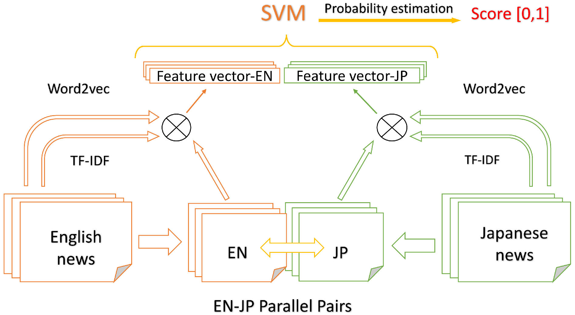
3.5. The SVM-Based Method

SVM is one of the most popular methods for solving both classification and regression tasks. It was originally purposed in 1990s and gradually proved to be effective in many fields including Natural language processing (NLP), pattern recognition and so on (Burges 1998; Malakasiotis and Androutsopoulos 2007; Béchara et al. 2015). TF-IDF and SVM are useful for tasks in the field of natural language processing. Therefore, we employ TF-IDF and SVM in our method as core technologies. Additionally, we propose a novel structure that uses TF-IDF and SVM effectively for this task. An overview of the structure is illustrated in Figure 1.
The system mainly contains three processing models. As our our training datasets, S only contains the data with label 0 or 1, the classification training objective of SVM is very similar to classification using Triplet Loss, which is proved to be quite effective in embedding and classification tasks (Schroff et al. 2015). The training procedures normally include the following steps:
  • Use the cross-lingual training data in the form of pre-trained word vectors as input, which is discussed in detail in Section 3.1.
  • Weight the word vectors for each of language models using TF-IDF, as introduced in Subsection 3.2 and Subsection 3.3.
  • Train the proposed model using SVM with Platt’s probability estimation for the connected cross-lingual document features, each of which are the naive join of two weighted word sum vectors in English and Japanese. This is explained in Section 3.4.

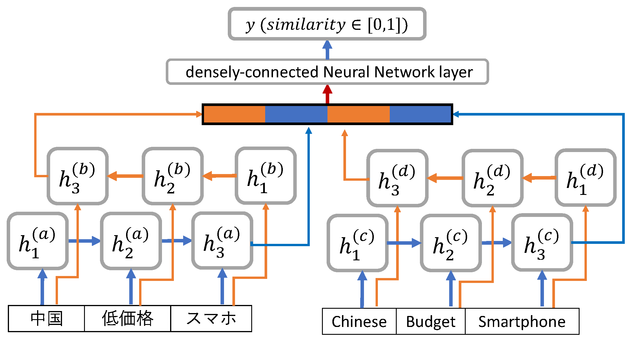
3.6. A Bidirectional LSTM Based Method

We implement the two independent modules of bi-directional LSTM recurrent neural networks on both English input and Japanese input respectively and the overview of this structure is shown in the Figure 2. We use the cross-lingual training data in the form of pre-trained word vectors as input. Feed the word vector sequentially to LSTM modules. This is discussed in detail in the Section 3.1. Furthermore, as a limitation of our LSTM modules, we have uniform length of data as input, denoted as “maxlen”. The residue of the parts of sequence longer than maxlen will be abandoned, while those with input sequence shorter than “maxlen” will be padded with a predefined value (i.e., a word) such as “null” at the tail so that all the input data could have the same length. The two bi-LSTM modules are responsible for the English sequence and Japanese Sequence respectively. They generate four hidden layer outputs and we concatenate them into a joint feature. Details are elaborated in the Section 3.6.1. The joined feature is further fed into a densely-connected neural network of 1 depth, resulting in 1 dimension output y [ 0 , 1 ] as the final similarity score of the two inputs of cross-lingual data, by means of regression. In general, the LSTM-based model pays more attention to the order information of the input sequence, which might significantly determine the real meaning of a sentence written in natural languages.

3.6.1. The Bi-LSTM Layer

In this research, we take advantage of bi-LSTM (bi-directional long short-term memory), to enhance the ordinary RNN performance considering both forward and backward information and solve the problem of the long-term dependencies. The updates rules of LSTM for each sequential input x 1 , x 2 , , x t , , x T could be express as:
i t = sigmoid ( W i x t + U i h t 1 + b i )
f t = sigmoid ( W f x t + U f h t 1 + b f )
c t ˜ = tanh ( W c x t + U c h t 1 + b c )
c t = i t c t ˜ + f t c t 1
o t = sigmoid ( W o x t + U o h t 1 + b o )
h t = o t tanh ( c t )
where h t 1 is the hidden layer value of the previous states and the sigmoid and tanh functions in the above equations are also used as activation functions:
sigmoid ( x ) = 1 1 + exp ( x )
tanh ( x ) = 2 1 + exp ( 2 x ) 1
The weights (i.e., parameters) we need to train include W i , W f , W c , W o , U i , U f , U c , U o and bias vectors b i , b f , b c , b o . A more thorough exposition of the LSTM model and its variants is provided by (Graves 2012) and (Greff et al. 2017). In this layer, we use the cross-lingual training data in the form of pre-trained word vectors as input, which is discussed in detail in Section 3.1. There are four LSTM modules, constructing two bi-LSTM structures, where we only consider the final output (i.e., final value of the hidden layer) of each LSTM module: LSTM-a read Japanese text in a forward direction. The value of a hidden layer is denoted as h i ( a ) where i is the i-th input of the sequence, while LSTM-b read backwards, denoted as h i ( b ) . Symmetrically, LSTM-c and LSTM-d are used to read English text, denoted as h i ( c ) and h i ( d ) . As the results, we obtain four feature vectors derived from hidden layer values of the four LSTM modules, keeping all necessary information regarding to the cross-lingual inputs. We then merge these four features by concatenating them directly:
x i , j = ( h L ( a ) , h L ( b ) , h L ( c ) , h L ( d ) )
where i and j refer to the document number of the input text for Japanese and English respectively, and vector h L ( a , b , c , d ) refers to the final status (i.e., the value) of the hidden layers of the LSTM module after feeding the last (or the first, if backwards) word.

3.6.2. Dense Layer

We use the most basic component of the basic full-dense Neural Network layer as the top layer. The function of this layer could be expressed as:
y i , j = f ( w T x i , j + b )
Here, the function f is also known as “activation” function, b is the one dimensional bias for the neural network and w is the weight (i.e., the parameters to be trained) of the neural network. In this project, we mainly apply the softplus Nair and Hinton (2010) function as the activation function in the dense layer:
f ( x ) = ln [ 1 + exp ( x ) ]
As for the optimization, although we are handling a classification problem, based on the experimental results, we find that, instead of using ordinary cross-entropy cost, it performs better if we use Quadratic cost (i.e., mean square error) as the cost function, which could be described as:
C = v = 1 N ( y t r u e , v y p r e d , v ) 2
where N is the total number of the training data, while y t r u e , v and y p r e d , v refer to the true similarity and the predicted similarity, respectively. In practice, the stochastic gradient descent (SGD) is implemented by means of the back-propagation scheme. After computing the outputs and errors based on the cost function J, which is usually equal to the negative log of the maximum likelihood function, we update parameters by the gradient descent method, expressed as:
w w ε w J ( w )
where ε is known as “learning rate”, defining the update speed of the hyper-parameters w . However, the training process might fail due to either improper initialization regarding weights or the improper learning rate value set. Practically, based on the results of the experiments, the best performance is achieved by applying the Adam optimizer Kingma and Ba (2014) to perform the parameter updates.

4. Experiments and Results

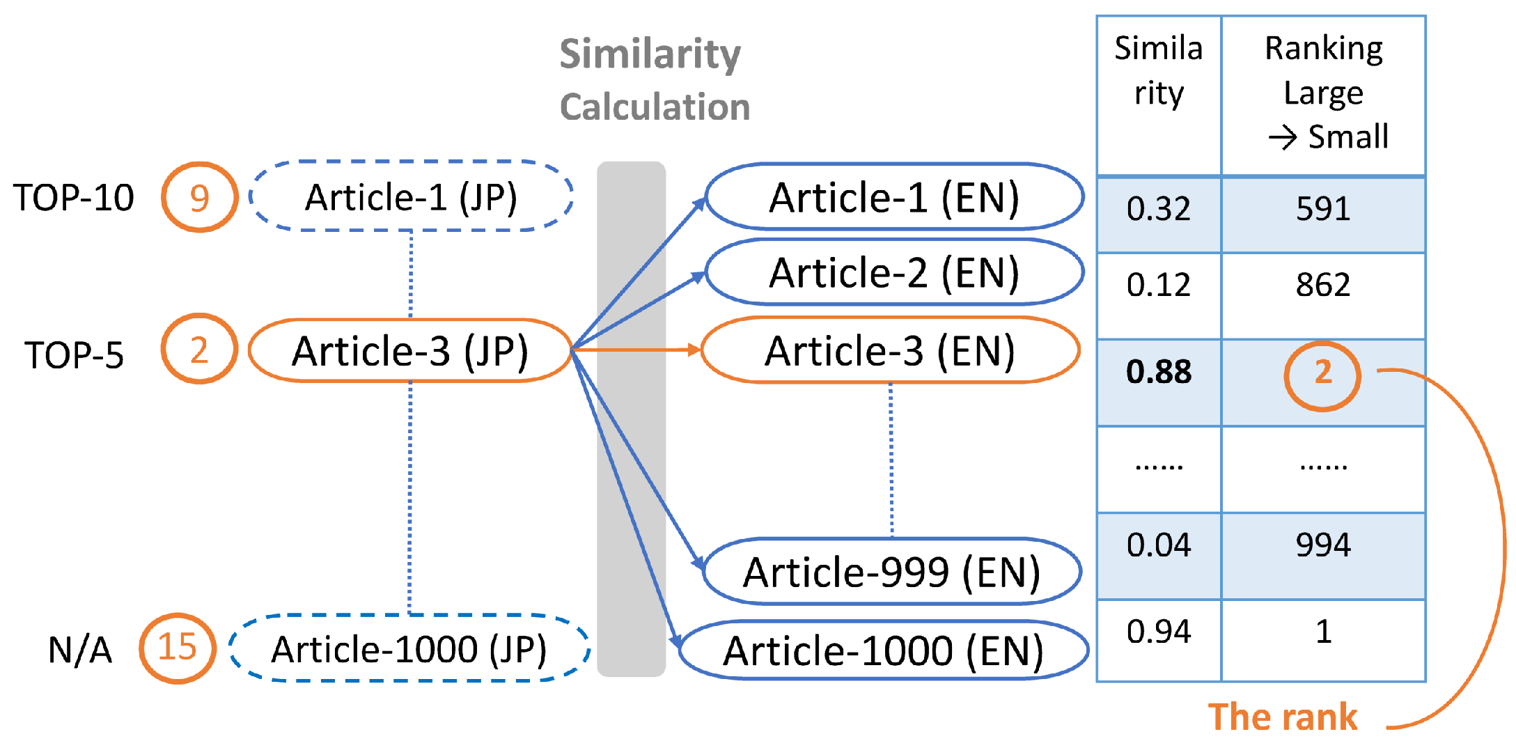
4.1. Evaluation Methods

We mainly use two categories of the evaluations, TOP-N benchmark based on ranks, and traditional criteria for classification such as precision, recall as well as the F1-value. As the applications of this project aim to suggest several cross-lingual (For instance, English) alternative news stories to the users, when the user provides a Japanese article as a query, we make the system pick up 1, 5 and 10 of the most similar Japanese alternatives during the evaluation process. The Figure 3 illustrates the relationship and evaluation procedures for ranks, TOP-N index.For a given Japanese text (i.e., the query) J x , calculate the similarity score between J x and all English text of test data sets ( E 1 , E 2 , , E x , , E M ) to derive a list of scores L x = ( S x , 1 , S x , 2 , , S x , x , , S x , M ) , where the corner mark M is the total number of English documents to be considered, and E x is the true similar article with a similarity score of 1. Then sort this list in the order from large to small and find out the rank (i.e., position, index) of the score S x , x inside this sorted list noted as R x , the rank for the query document J x . Repeat this process recursively for N Japanese articles ( J 1 , J 2 , , J N ) , result in a list of ranks R = ( R 1 , R 2 , , R N ) regarding the collections of J x . Then we take the number of query documents with ranks smaller than N as TOP-N. In other words, TOP-1 refers to the number of query documents with rank equal to 1 and TOP-5 refers to the number of a query with rank equal to or smaller than 5.

4.2. Baseline: Siamese LSTM with Google-Translation

Siamese LSTM is one of the deep learning-based models with the art-of-state performance on the semantic text similarity problems. In this research, we make this model a baseline by extending this model from a monolingual domain to a cross-lingual domain with the help of the Google Translation services. We first translate all Japanese text into the English version on both test and training data by using the google translate service1 Then we implement the Siamese LSTM model as described in the original paper for Siamese LSTM Mueller and Thyagarajan (2016) with the help of the open source code on the Github2 To illustrate this baseline method regarding a two cross-lingual input, we first translate the Japanese input into an English sentence using Google Translation service. Then, we can consider the cross-lingual task as monolingual one so that we can apply the Siamese LSTM model for training as a baseline.

4.3. Datasets and Pre-Processing

Thomson Reuters news3 is a worldwide news agency providing worldwide news in multiple languages. Most of the reports are originally written in English and translated and edited into other languages including Chinese, Japanese, etc. These multi-lingual texts are expected to be highly potential resources for tasks related to the multi-lingual natural languages processing. In this research, we use 60,000 news articles in 2014 from Thomson Reuters News related to the economics. For the preprocessing of text, we convert raw data to normalized data, which could be further used to train word2vec models for both English and Japanese text, respectively. We train the Japanese word2vec model and English word2vec model separately using news articles with the same contents in 2014. In our experiment, we use the model of a Continuous Bag of Words (CBOW), with 200 fixed dimensions of word embedding. Other parameters are set using the default value used in the Gensim package4.
As discussed in Section 3.1, the word2vec could build relationships among words based on their original context. We could find several of the most similar words when given a query word by calculating their cosine similarity. The Table 1 and Table 2 demonstrate examples to find the most similar words when given a word query in English and in Japanese respectively. All these results suggest the effectiveness of word2vec algorithms and success of the training processes.

4.4. Experiments on Text Datasets

4.4.1. Training Data

Regarding Short Text, we firstly pick up 4000 pairs of parallel Japanese-English cross-lingual news titles from the database with the period from the January to February of 2014, all of which are labeled with a similarity score of 1. To provide balance training data, we also generated 4000 pairs of un-parallel Japanese-English cross-lingual news titles by a random combination. In order to simplify our model and experiments, we use the assumption that the similarity the random combination of Japanese text and English text is 0. Then, for Long Text, similar to the data preparation of experiments for short text introduced, we prepare 4000 parallel (i.e., similarity = 1) Japanese-English news articles and 4000 un-parallel (i.e., similarity = 0) ones for training data through random combination.

4.4.2. Test Data

For Short Text, in order to evaluate our model more comprehensively, we have prepared two sets of independent test data. TEST-1S contains 1000 pairs of parallel Japanese-English news titles, selected and split from the same period of training data, from January 2014 to the middle of February in 2014. Similarly, TEST-2S contains title pairs with time stamps of December 2014. For Long Text, similar to the case of short test evaluation, we have prepared two sets of independent test data. For training data, we prepared a similar dataset as for the short text experiments. TEST-1L and TEST-2L contain 1000 pairs of parallel Japanese-English long news articles respectively.

4.4.3. Ranks and TOP-N

Table 3 also summarizes and compares our two purposed models, LSTM-based model and SVM-based model respectively in terms of TOP-N benchmark regarding LONG text scenario and SHORT text scenario.
First, we could notice that both our purposed, LSTM-based model and SVM-based model, outperform the baseline in terms of all three TOP-N criteria. In terms of TOP-N, the LSTM-based model obtains around twice the performance of the baseline (511 vs. 243) on short test data, while LSTM-based model also has twice the performance of the baseline (685 vs. 302) on long test data, suggesting the effectiveness and efficiency of our purposed models. Furthermore, we may also easily notice that the SVM-based method outperforms the LSTM-based methods in terms of TOP-N criteria, in case of long text, around 50%. In contrast, the LSTM-based model has a TOP-10 score around 10% higher than that of the SVM-based model on both test datasets.
The dominant performance of the SVM-based model on long test data is also maintained in terms of TOP-1 and TOP-5, twice the score compared to the LSTM-based model for TOP-5 and three times the score for the TOP-1 benchmark. On the other hand, although the LSTM-based model still performs better than SVM-based with respect to TOP-5, as for TOP-5 LSTM-based model failed to be in the lead anymore. We are going to discuss these results and propose possible hypotheses and provide explanations in Section 5. The performance of successful recommendation numbers from our bi-LSTM based model is twice that of the baseline.

5. Discussion

5.1. Comparison of the Baseline and the LSTM-Based Model

The performance of the LSTM-based model is twice that of the baseline, even though they are both based on LSTM structures. The differences, which are also the innovations for this purposed method, compared to the baseline, include the using of bi-LSTM, independent LSTM modules as well as using the fully connected neural network as the final layer.
First, the baseline method is able to calculate the similarity of two sentences, no matter whether there are different types of word arrangement for the two inputs, or if there are different words used referring to the same meaning, which proves the effectiveness of the encoding (i.e., embedding) ability for the input text. However, the baseline model has the “Siamese LSTM structure”, which means, in other words, that the two LSTM instances always share the same parameters during the training. This might be effective for a monolingual case, but not good enough on the cross-lingual case. Thus, the LSTM instances used in our purposed model are all independently holding their own unique parameters. In addition, the bi-directional structure also helps to encode the feature of each input text more comprehensively. Finally, instead of using cosine similarity as the final layer in the baseline method, we used the fully connected neural network as output, making the output layer adjust (i.e., train) its parameters so as to learn precise patterns from the features generated by LSTMs. We believe these three modifications improve the final results for our LSTM-based model.

5.2. Comparison of the LSTM-Based Model and SVM-Based Model

The experiments above leave us with an interesting question about why the LSTM-based model and SVM-based model perform differently regarding the length of the target text we train and test. We explain this question in two aspects.

5.2.1. From the Point of View of the SVM-Based Model

Since the SVM-based methods use the TF-IDF weighting which is a classical and an effective method for NLP fields to extract the most important and representative features for each of document comprehensively, it could accurately identify the most significant feature, a few key words, from a very long and complex article containing hundreds of words, in both Japanese and English, and then finally feed them into the SVM classifier to get the similarity estimation universally. However, due to the attributes of TF-IDF algorithms, the shorter the length of each document is, the less information the TF-IDF could extract. This is because if there are fewer words in one document, every word could be either unique or common regarding other documents, resulting in the failure of TF-IDF. This might be the reason why SVM-based model performs well on long datasets but this performance becomes poor on shorter data sets.

5.2.2. From the Point of View of the LSTM-Based Model

On the other hand, the LSTM is good at understanding sentences by means of grasping the order information of each words, since for any natural languages, not only words themselves but also the order of words, to some extent, define the true meaning of a sentence. Especially for short text, a slight change of the order could alter the meaning of the sentences significantly and thus the LSTM-based model outperformed the LSTM model by around 10% on short datasets. However, LSTM is not good at extracting the key idea of longer documents since, although LSTM solves the problem of memorizing long text (i.e., solve of the problem of gradient vanishing and gradient explosion), it could tell the importance of each word as TF-IDF does. That might be the possible reason why it fails to perform effectively on a long text.

6. Conclusions

We developed a bi-LSTM-based model to calculate cross-lingual similarities given a pair of English and Japanese articles. Instead of using a translation module or a dictionary to translate from one to another language, our model has outstanding performance with short text. Furthermore, we modified and implemented a popular Siamese LSTM model as the baseline and we found both of our models outperform the baseline. For practical testing, we defined the concept of “TOP-N” and “ranks” to test the overall performance of the model, with visualized results. We also make a comparative study based on the results of the experiments that bi-LSTM based obtains better performance on short text data such as news titles and alert messages, which are on average shorter than 20 words, in contrast to normal news articles with more than 200 words on average. As the results show, both models obtained satisfactory performance with over half of the test documents of 1000 holding ranks lower than 10 (i.e., TOP-10). As a high-performance cross-lingual news calculating system, we expect that it could achieve optimal performance by taking advantage of both models to form a complete system.

Supplementary Materials

The following are available online at https://www.mdpi.com/1911-8074/11/1/8/s1.
Supplementary File 1

Acknowledgments

Thanks three anonymous reviewers from JRFM for reviewing our paper, and providing valuable instructions to revise our paper.

Author Contributions

Zhouhao Wang, Enda Liu and Hiroki Sakaji conceived and designed the experiments. Enda Liu performed the experiments. Zhouhao Wang and Enda Liu analyzed the data. Tomoki Ito, Kiyoshi Izumi, Kota Tsubouchi and Tatsuo Yamashita contributed materials. Zhouhao Wang, Hiroki Sakaji and Kiyoshi Izumi wrote the paper.

Conflicts of Interest

The authors declare no conflict of interest.

References

  1. Agirrea, Eneko, Carmen Baneab, Daniel Cerd, Mona Diabe, Aitor Gonzalez-Agirrea, Rada Mihalceab, German Rigaua, and Janyce Wiebe. 2016. Semeval-2016 task 1: Semantic textual similarity, monolingual and cross-lingual evaluation. Paper presented at the SemEval-2016, San Diego, CA, USA, June 16–17; pp. 497–511. [Google Scholar]
  2. Baroni, Marco, Georgiana Dinu, and German Kruszewski. 2014. Don’t count, predict! a systematic comparison of context-counting vs. context-predicting semantic vectors. Paper presented at the 52nd Annual Meeting of the Association for Computational Linguistics, Baltimore, MD, USA, June 23–25; pp. 238–47. [Google Scholar]
  3. Béchara, Hanna, Hernani Costa, Shiva Taslimipoor, Rohit Gupta, Constantin Orasan, Gloria Corpas Pastor, and Ruslan Mitkov. 2015. Miniexperts: An svm approach for measuring semantic textual similarity. Paper presented at the 9th International Workshop on Semantic Evaluation (SemEval 2015), Denver, CO, USA, June 4–5; pp. 96–101. [Google Scholar]
  4. Burges, Christopher J. C. 1998. A tutorial on support vector machines for pattern recognition. Data Mining and Knowledge Discovery 2: 121–67. [Google Scholar] [CrossRef]
  5. Gouws, Stephan, Yoshua Bengio, and Greg Corrado. 2015. Bilbowa: Fast bilingual distributed representations without word alignments. Paper presented at the 32nd International Conference on Machine Learning (ICML-15), Lille, France, July 7; pp. 748–56. [Google Scholar]
  6. Graves, Alex. 2012. Supervised Sequence Labelling with Recurrent Neural Networks. Berlin and Heidelberg: Springer, vol. 385. [Google Scholar]
  7. Greff, Klaus, Rupesh K. Srivastava, Jan Koutník, Bas R. Steunebrink, and Jürgen Schmidhuber. 2017. Lstm: A search space odyssey. IEEE Transactions on Neural Networks and Learning Systems 28: 2222–32. [Google Scholar] [CrossRef] [PubMed]
  8. Hochreiter, Sepp, and Jürgen Schmidhuber. 1997. Long short-term memory. Neural Computation 9: 1735–80. [Google Scholar] [CrossRef] [PubMed]
  9. Kingma, Diederik P., and Jimmy Ba. 2014. Adam: A Method for Stochastic Optimization. Available online: https://arxiv.org/abs/1412.6980 (accessed on 16 August 2017).
  10. Kudo, Taku, Kaoru Yamamoto, and Yuji Matsumoto. 2004. Applying conditional random fields to japanese morphological analysis. Paper presented at the 2004 Conference on Empirical Methods in Natural Language Processing, Barcelona, Spain, July 25; vol. 4, pp. 230–37. [Google Scholar]
  11. Le, Quoc, and Tomas Mikolov. 2014. Distributed representations of sentences and documents. Paper presented at the 31st International Conference on Machine Learning (ICML-14), Beijing, China, June 23; pp. 1188–96. [Google Scholar]
  12. Lo, Chi-kiu, Meriem Beloucif, Markus Saers, and Dekai Wu. 2014. Xmeant: Better semantic mt evaluation without reference translations. Paper presented at the 52nd Annual Meeting of the Association for Computational Linguistics (Volume 2: Short Papers), Baltimore, MD, USA, June 23–25; vol. 2, pp. 765–71. [Google Scholar]
  13. Malakasiotis, Prodromos, and Ion Androutsopoulos. 2007. Learning textual entailment using svms and string similarity measures. Paper presented at the ACL-PASCAL Workshop on Textual Entailment and Paraphrasing, Prague, Czech Republic, June 28–29; Stroudsburg: Association for Computational Linguistics, pp. 42–47. [Google Scholar]
  14. Mikolov, Tomas, Ilya Sutskever, Kai Chen, Greg Corrado, and Jeffrey Dean. 2013. Distributed representations of words and phrases and their compositionality. Paper presented at the 26th International Conference on Neural Information Processing Systems, Lake Tahoe, NV, USA, December 5–10; pp. 3111–19. [Google Scholar]
  15. Mueller, Jonas, and Aditya Thyagarajan. 2016. Siamese recurrent architectures for learning sentence similarity. Paper presented at the 30th AAAI Conference on Artificial Intelligence (AAAI 2016), Phoenix, AZ, USA, February 16; pp. 2786–92. [Google Scholar]
  16. Nair, Vinod, and Geoffrey E. Hinton. 2010. Rectified linear units improve restricted boltzmann machines. Paper presented at the 27th International Conference on Machine Learning (ICML-10), Haifa, Israel, June 21–24; pp. 807–14. [Google Scholar]
  17. Rupnik, Jan, Andrej Muhic, Gregor Leban, Blaz Fortuna, and Marko Grobelnik. 2016. News across languages-cross-lingual document similarity and event tracking. Journal of Artificial Intelligence Research 55: 283–316. [Google Scholar]
  18. Schroff, Florian, Dmitry Kalenichenko, and James Philbin. 2015. Facenet: A unified embedding for face recognition and clustering. In Paper presented at Proceedings of the IEEE Conference on Computer Vision and Pattern Recognition, Boston, MA, USA, June 7–12; pp. 815–23. [Google Scholar]
  19. Taghva, Kazem, Rania Elkhoury, and Jeffrey Coombs. 2005. Arabic stemming without a root dictionary. Paper presented at International Conference on Information Technology: Coding and Computing, 2005 (ITCC 2005), Las Vegas, NV, USA, April 4–6; vol. 1, pp. 152–157. [Google Scholar]
  20. Tang, Duyu, Furu Wei, Nan Yang, Ming Zhou, Ting Liu, and Bing Qin. 2014. Learning sentiment-specific word embedding for twitter sentiment classification. Paper presented at the 52nd Annual Meeting of the Association for Computational Linguistics, Baltimore, MD, USA, June 23–25; pp. 1555–65. [Google Scholar]
  21. Zou, Will Y., Richard Socher, Daniel Cer, and Christopher D. Manning. 2013. Bilingual word embeddings for phrase-based machine translation. Paper presented at the 2013 Conference on Empirical Methods in Natural Language Processing, Seattle, WA, USA, October 19; pp. 1393–98. [Google Scholar]
1
Google Translation Web API could be accessed from https://github.com/aditya1503/Siamese-LSTM.
2
The open source code for Siamese LSTM can be accessed from https://github.com/aditya1503/Siamese-LSTM.
3
Official websites of Thomson Reuters: http://www.reuters.com/.
4
To see more specific of the configuration of word2vec model, see the documentation of Word2Vec class from https://radimrehurek.com/gensim/models/word2vec.html.
Figure 1. Illustration of our SVM-based method.
Jrfm 11 00008 g001
Figure 2. Illustration of the LSTM-based method.
Jrfm 11 00008 g002
Figure 3. Illustration of an evaluation procedures using ranks and TOP-N index.
Jrfm 11 00008 g003
Table 1. Example of similarity relationship for Japanese words (translated).
ToyotaSony
TOPWordSimilarityWordSimilarity
1Honda0.612PlayStation0.612
2Toyota corp0.546Entertainment0.546
3Hyundai corp0.536SonyBigChance0.536
4Chrysler0.524Game console0.524
5Nissan0.519Nexus0.519
6motor0.511X-BOX0.511
7LEXUS0.506spring0.506
8Acura0.493Windows0.493
9Mazda0.492Compatibility0.492
10Ford0.486application software0.486
Table 2. Example of similarity relationship for English words.
LexusLenovo
TOPWordSimilarityWordSimilarity
1acura0.636huawei0.636
2corolla0.588zte0.588
3camry0.571xiaomi0.571
42002–20050.570dell0.570
5sentra0.541handset0.541
6prius0.539smartphone0.539
72003–20050.537hannstar0.537
8sedan0.533thinkpad0.533
9mazda0.530tcl0.530
10altima0.524medison0.524
Table 3. Summary of in terms of TOP-N benchmark.
TOP-10
SHORTLONG
TEST-1STEST-2STEST-1LTEST-1L
LSTM511495456432
SVM453422685654
baseline243-302-
TOP-5
SHORTLONG
TEST-1STEST-2STEST-1LTEST-1L
LSTM339338284278
SVM324295520491
baseline134-192-
TOP-1
SHORTLONG
TEST-1STEST-2STEST-1LTEST-1L
LSTM901066158
SVM10196128179
baseline39-50-

