Application of Functional Data Analysis to Identify Patterns of Malaria Incidence, to Guide Targeted Control Strategies

 , ,
, ,  ,
,
Abstract
:1. Introduction
2. Methods
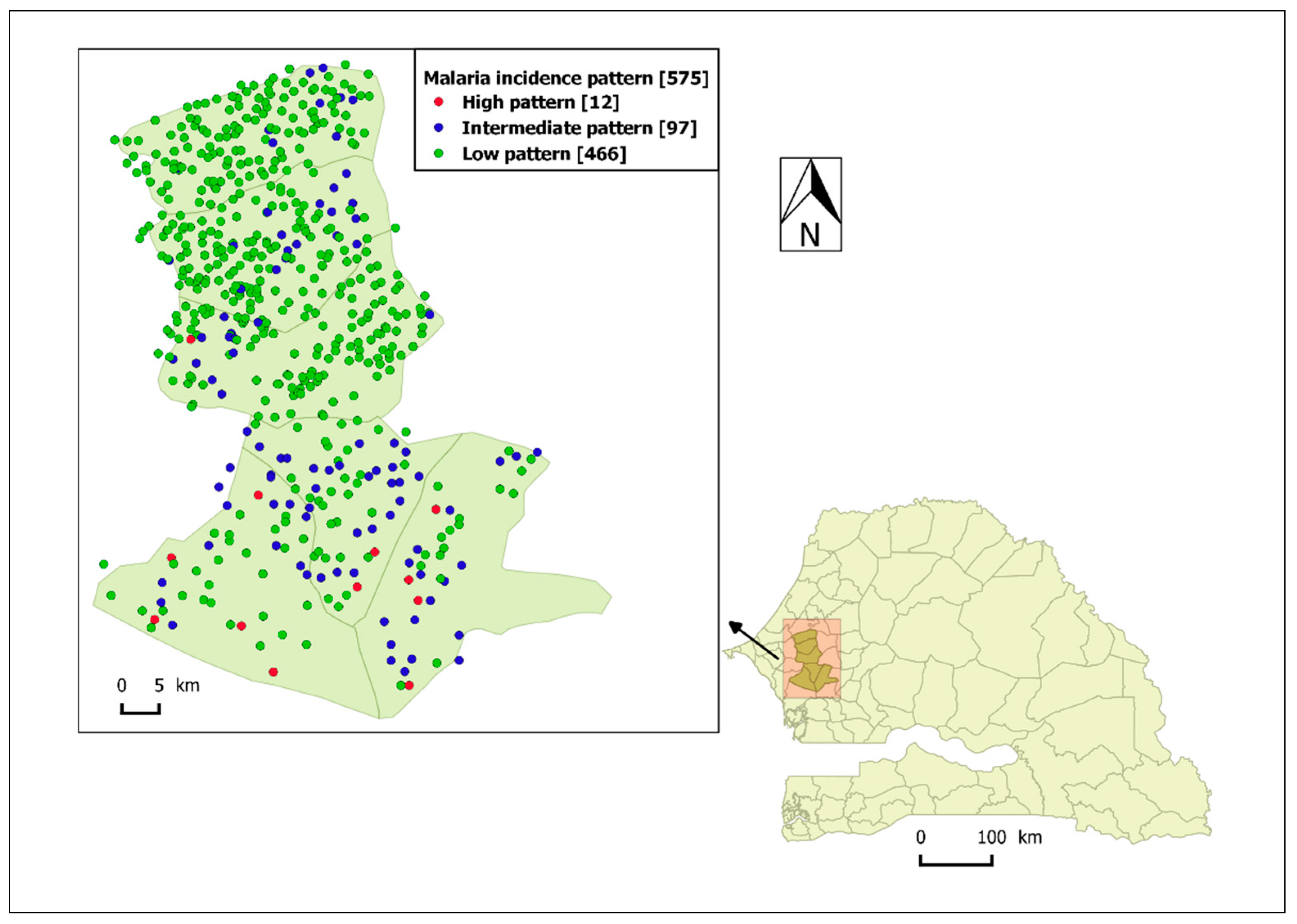
2.1. Study Area and Dataset
2.2. Statistical Analysis
2.2.1. Estimating the Smooth Function (Functional Data) for Each Time Series
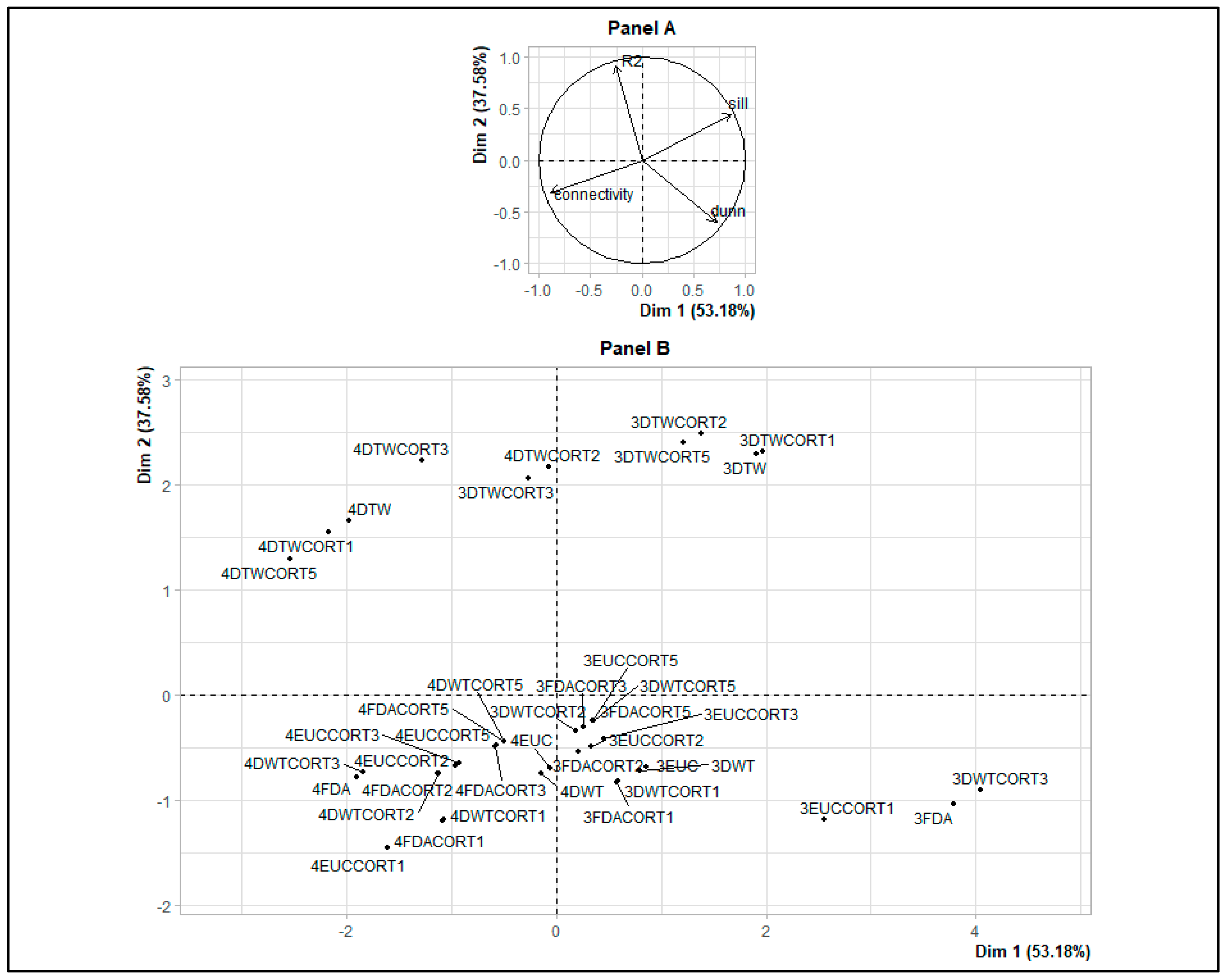
2.2.2. Dissimilarity Measures and Hierarchical Ascending Clustering on Smooth Functions
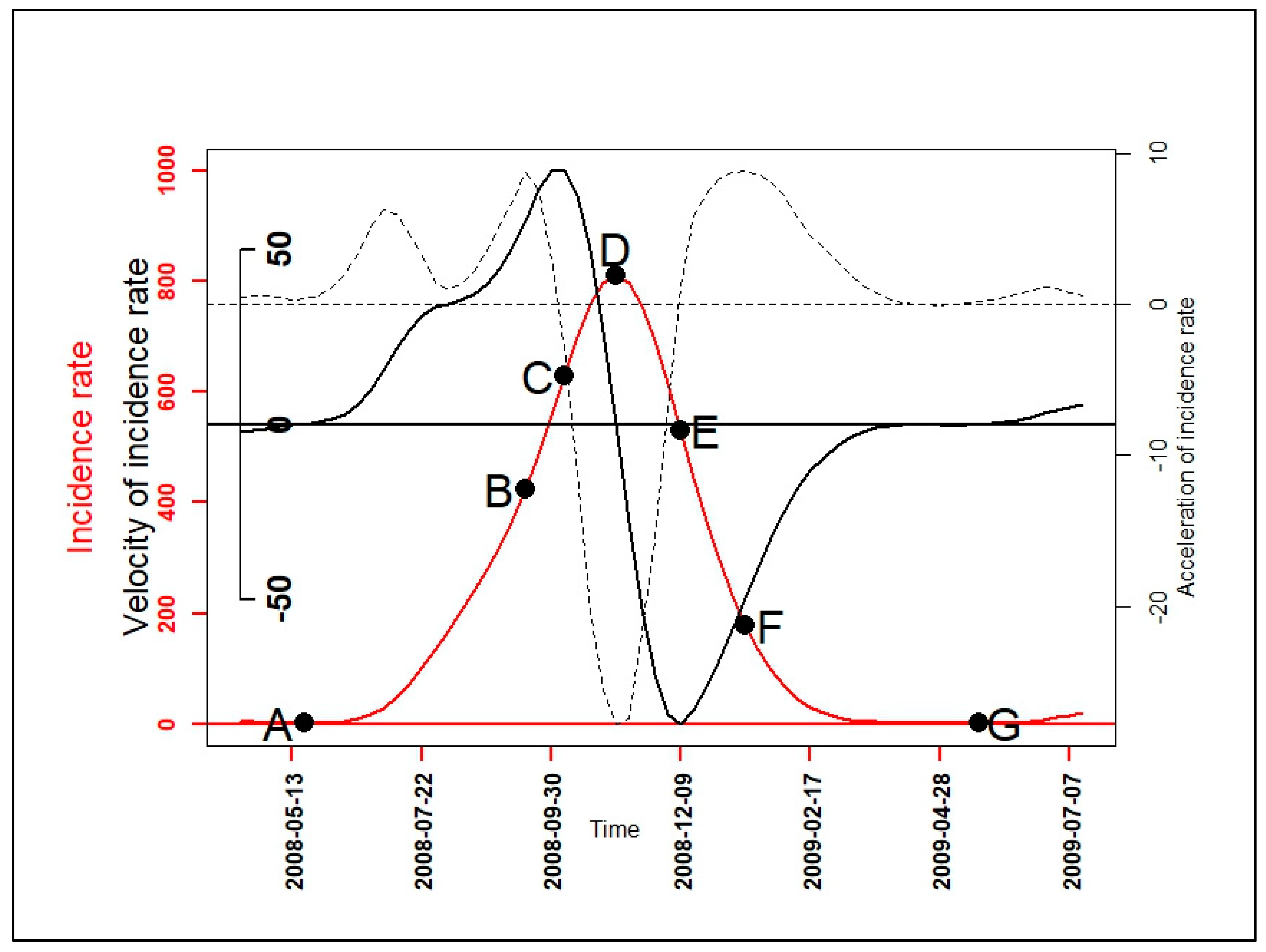
2.2.3. Velocity and Acceleration
3. Results
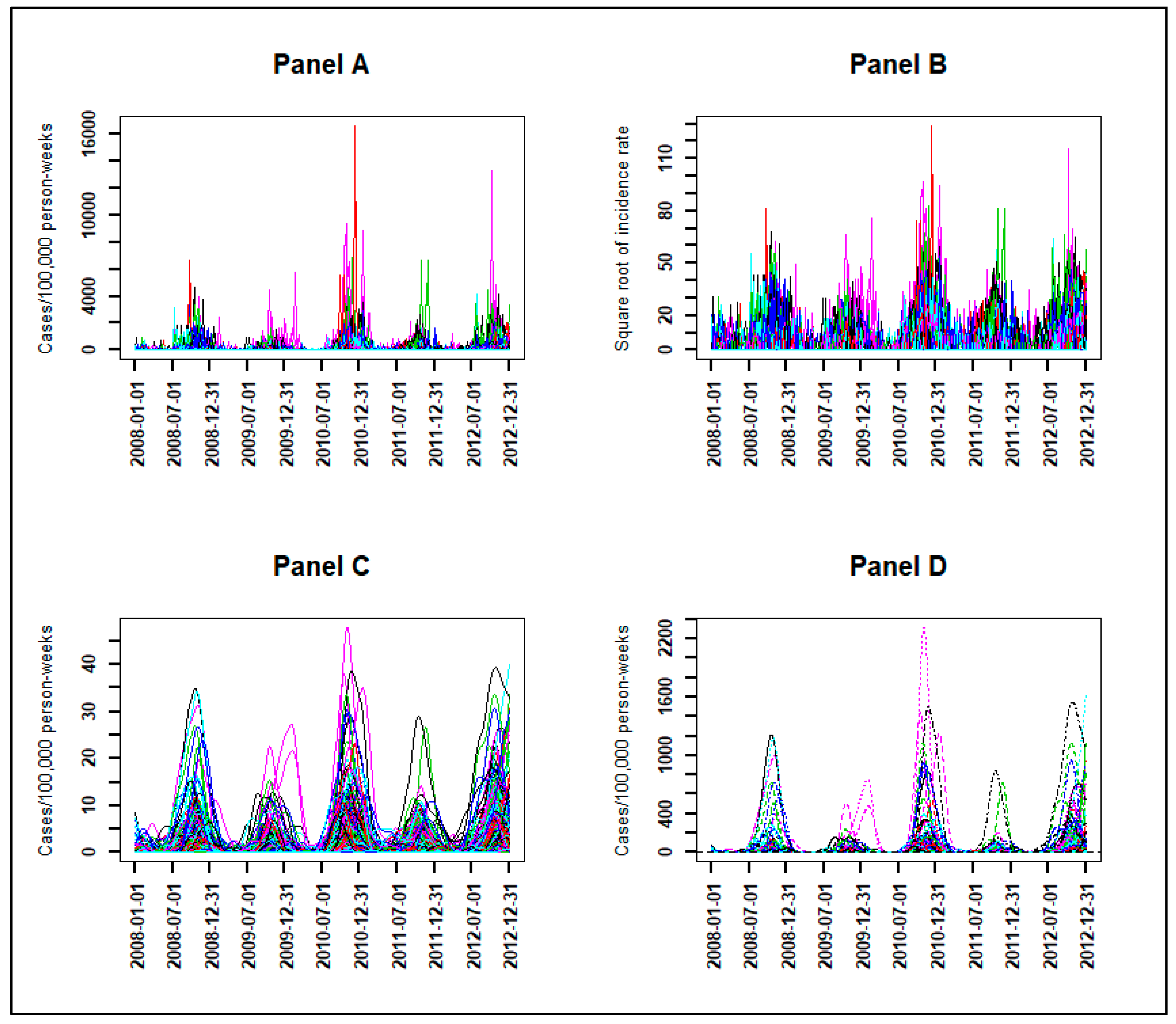
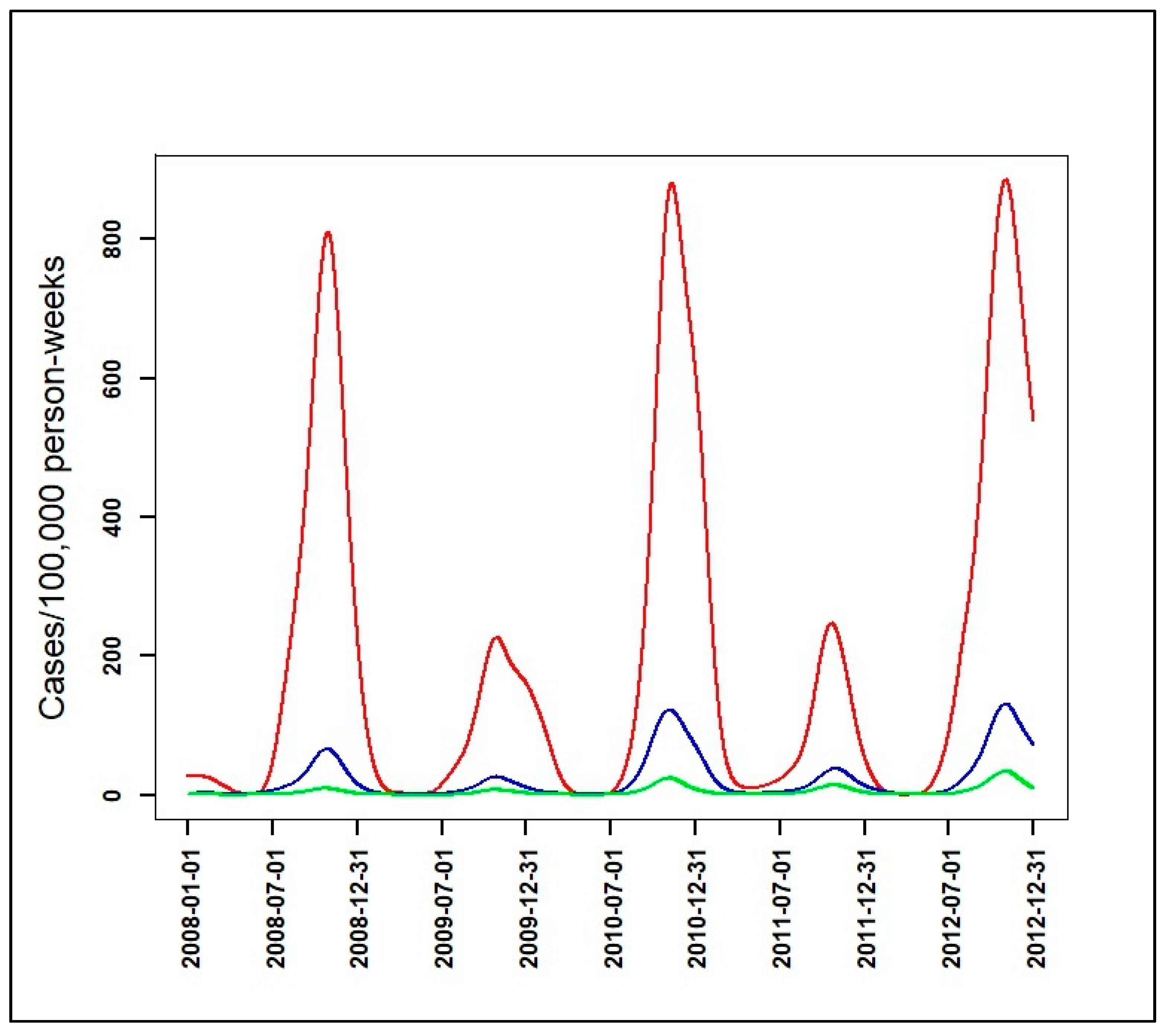
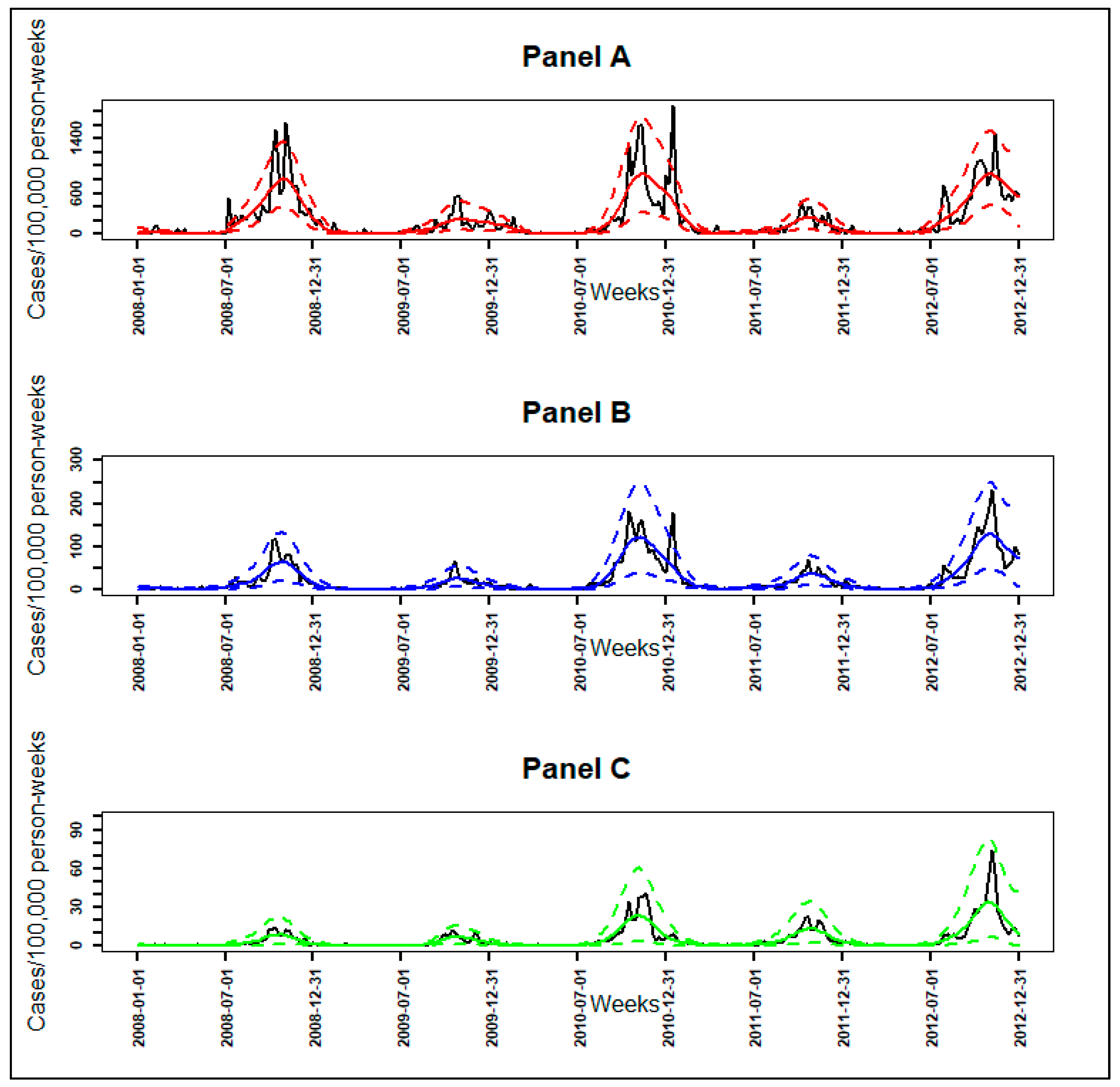
3.1. From Observed to Smoothed Malaria Incidence
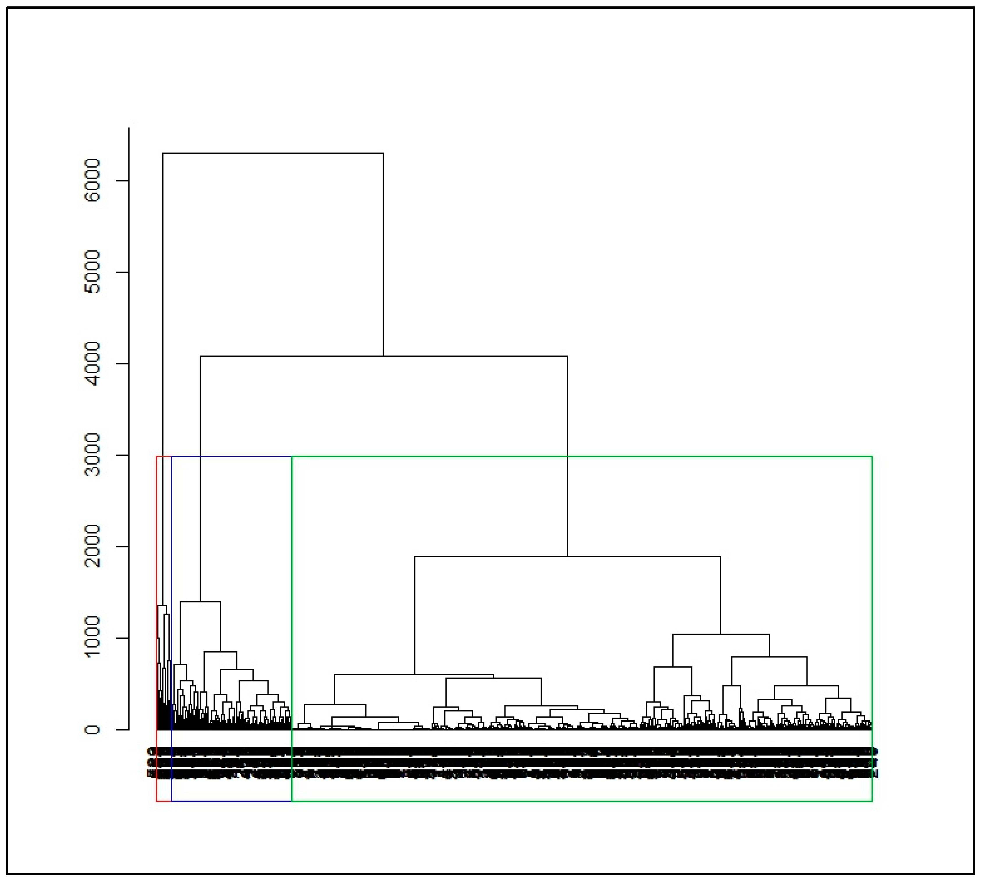
3.2. Identification of Malaria Incidence Patterns
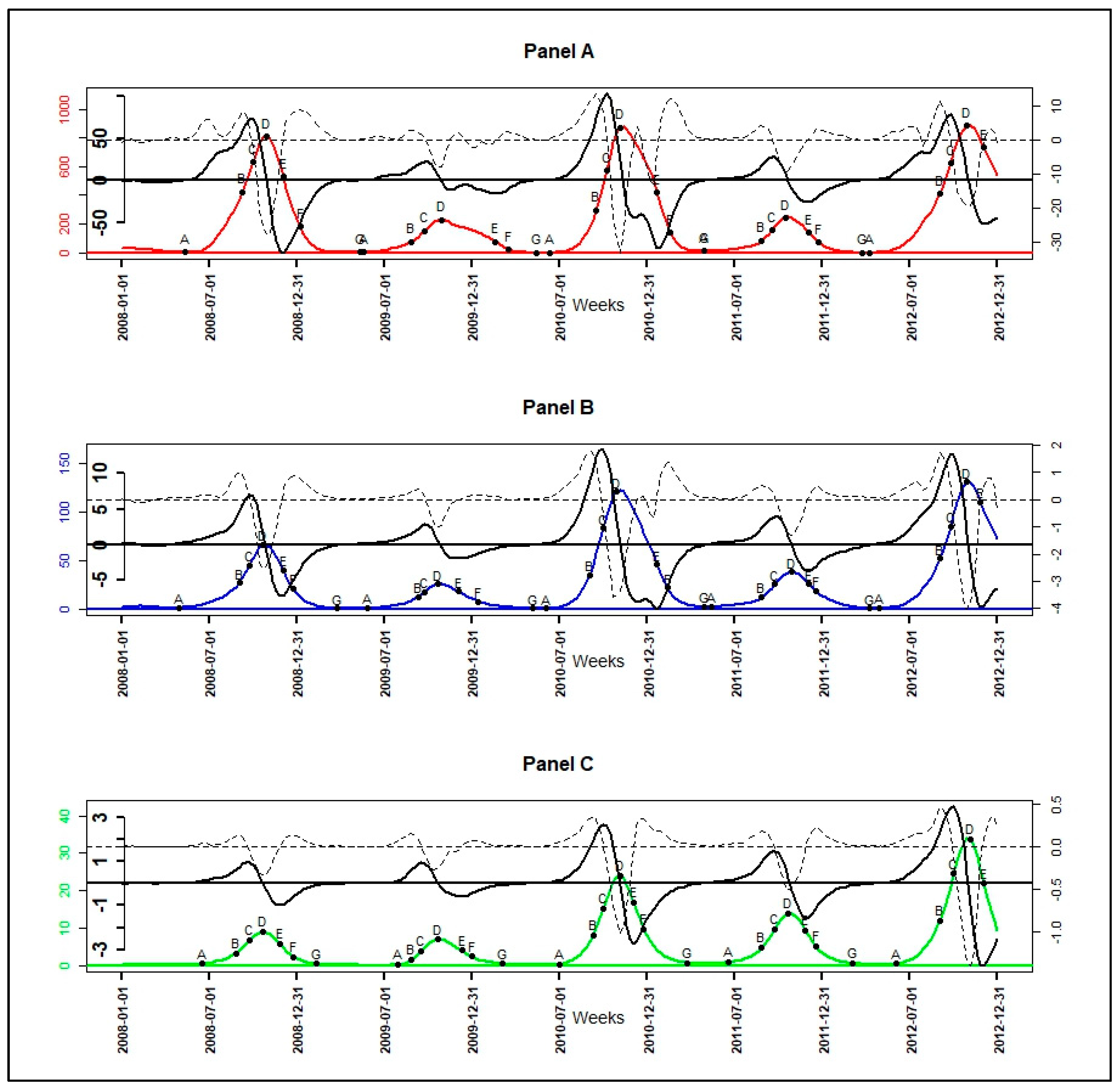
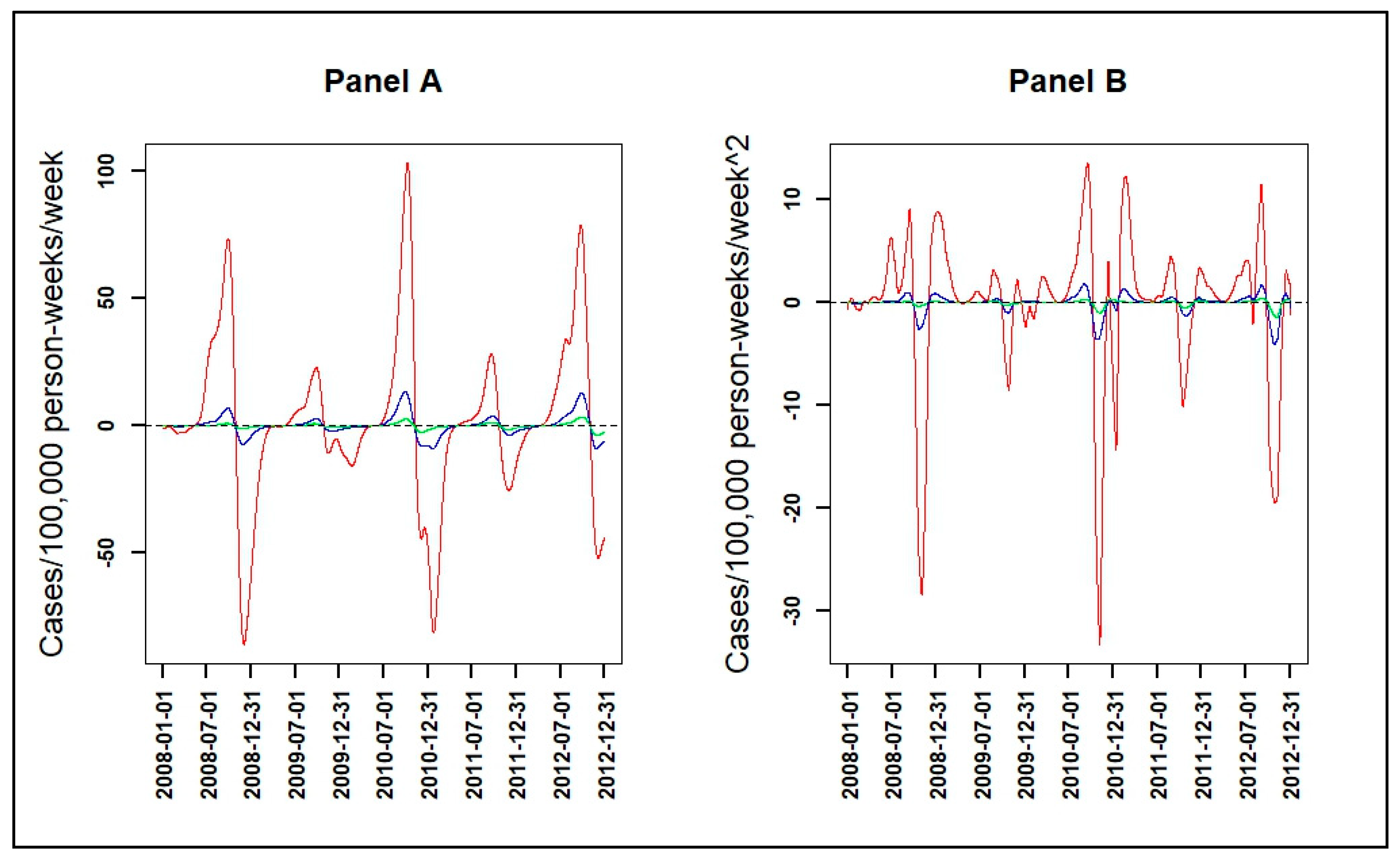
3.3. Velocity and Acceleration of Malaria Incidence Patterns
4. Discussion
5. Conclusions
Author Contributions
Funding
Acknowledgments
Conflicts of Interest
Appendix A

| HAC Results (with 3 and 4 Clusters) and Dissimilarity Measures | Connectivity | Dunn | Silhouette | R2 |
|---|---|---|---|---|
| 3EUC | 113.57 | 0.04 | 0.38 | 0.1 |
| 3FDA | 73.44 | 0.08 | 0.52 | 0.1 |
| 3DTW | 80.47 | 0.03 | 0.55 | 0.19 |
| 3DWT | 112.88 | 0.04 | 0.37 | 0.1 |
| 3EUCCORT1 | 102.07 | 0.07 | 0.46 | 0.1 |
| 3EUCCORT2 | 117.83 | 0.03 | 0.36 | 0.1 |
| 3EUCCORT3 | 118.87 | 0.03 | 0.38 | 0.1 |
| 3EUCCORT5 | 122.23 | 0.03 | 0.38 | 0.11 |
| 3FDACORT1 | 121.69 | 0.04 | 0.36 | 0.1 |
| 3FDACORT2 | 124.79 | 0.03 | 0.36 | 0.1 |
| 3FDACORT3 | 118.93 | 0.03 | 0.36 | 0.11 |
| 3FDACORT5 | 121.7 | 0.03 | 0.38 | 0.11 |
| 3DWTCORT1 | 121.06 | 0.04 | 0.36 | 0.1 |
| 3DWTCORT2 | 123.79 | 0.03 | 0.36 | 0.11 |
| 3DWTCORT3 | 66.56 | 0.08 | 0.54 | 0.1 |
| 3DWTCORT5 | 121.55 | 0.03 | 0.38 | 0.11 |
| 3DTWCORT1 | 76.4 | 0.03 | 0.55 | 0.19 |
| 3DTWCORT2 | 84.01 | 0.02 | 0.53 | 0.19 |
| 3DTWCORT3 | 109.12 | 0.01 | 0.4 | 0.19 |
| 3DTWCORT5 | 89.88 | 0.02 | 0.52 | 0.19 |
| 4EUC | 149.3 | 0.04 | 0.35 | 0.12 |
| 4FDA | 158.82 | 0.02 | 0.2 | 0.12 |
| 4DTW | 174.53 | 0.01 | 0.33 | 0.21 |
| 4DWT | 149.92 | 0.04 | 0.34 | 0.12 |
| 4EUCCORT1 | 206.79 | 0.04 | 0.27 | 0.12 |
| 4EUCCORT2 | 171.17 | 0.03 | 0.32 | 0.12 |
| 4EUCCORT3 | 173.47 | 0.03 | 0.33 | 0.12 |
| 4EUCCORT5 | 156.54 | 0.03 | 0.34 | 0.12 |
| 4FDACORT1 | 188.3 | 0.04 | 0.3 | 0.12 |
| 4FDACORT2 | 181.55 | 0.03 | 0.32 | 0.12 |
| 4FDACORT3 | 157.83 | 0.03 | 0.34 | 0.12 |
| 4FDACORT5 | 156.44 | 0.03 | 0.35 | 0.12 |
| 4DWTCORT1 | 187.75 | 0.04 | 0.3 | 0.12 |
| 4DWTCORT2 | 180.55 | 0.03 | 0.32 | 0.12 |
| 4DWTCORT3 | 163.1 | 0.02 | 0.22 | 0.12 |
| 4DWTCORT5 | 156.27 | 0.03 | 0.35 | 0.12 |
| 4DTWCORT1 | 177.8 | 0.01 | 0.31 | 0.21 |
| 4DTWCORT2 | 126.73 | 0.02 | 0.44 | 0.21 |
| 4DTWCORT3 | 151.85 | 0.01 | 0.38 | 0.22 |
| 4DTWCORT5 | 166.42 | 0.01 | 0.23 | 0.21 |


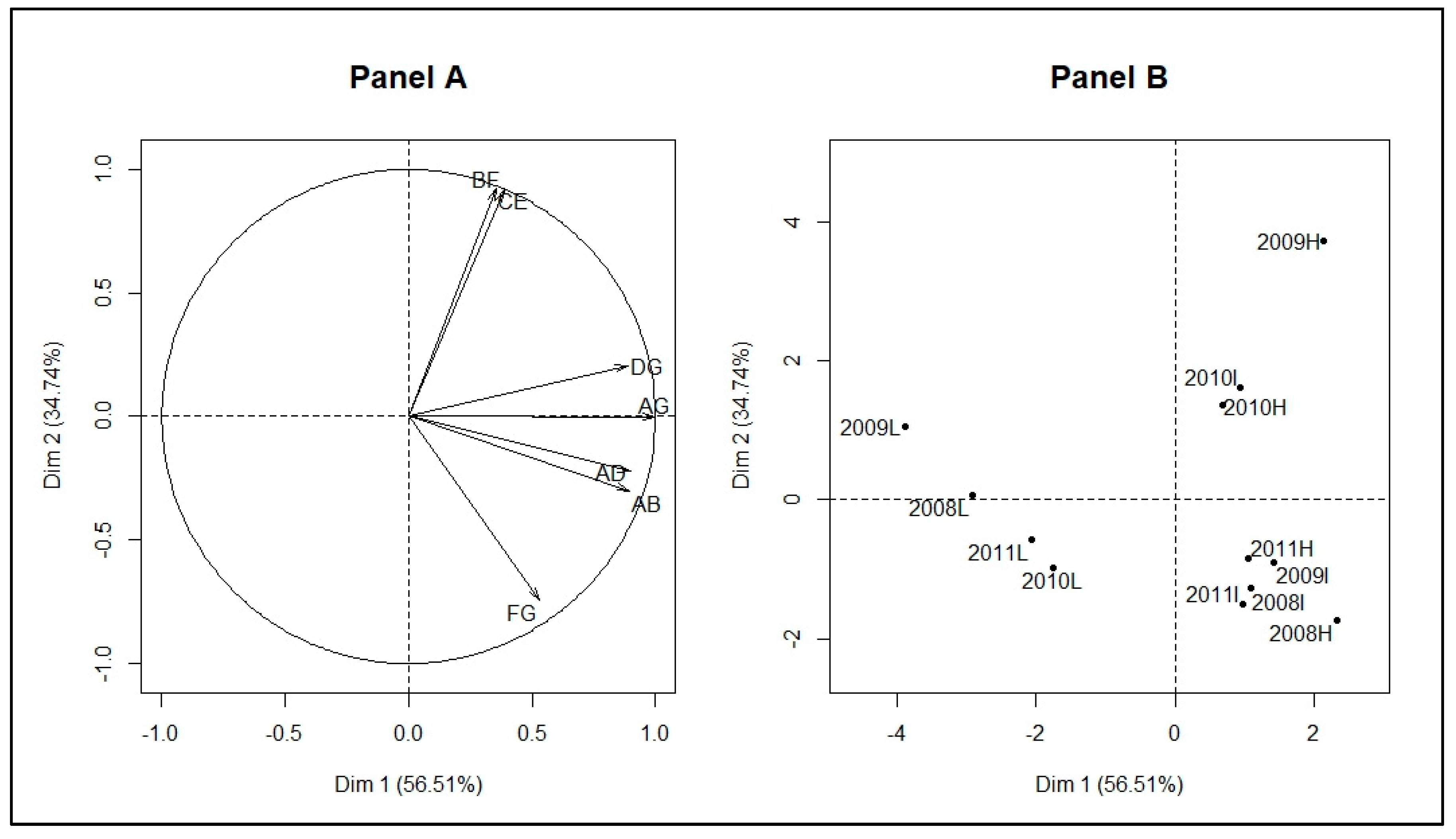
| PCA_Indicators | Dim.1 | Dim.2 | Dim.3 | Dim.4 | Dim.5 |
|---|---|---|---|---|---|
| correlation_AB | 0.9 | −0.3 | −0.31 | −0.08 | −0.06 |
| correlation _AD | 0.9 | −0.22 | −0.37 | 0.08 | 0.05 |
| correlation _CE | 0.35 | 0.92 | 0 | 0.13 | −0.07 |
| correlation _DG | 0.89 | 0.21 | 0.4 | −0.09 | −0.02 |
| correlation _FG | 0.53 | −0.74 | 0.39 | 0.11 | 0.01 |
| correlation _BF | 0.39 | 0.92 | 0.03 | −0.03 | 0.08 |
| correlation _AG | 1 | 0 | 0.03 | −0.01 | 0.02 |
| cosinus2_AB | 0.8 | 0.09 | 0.1 | 0.01 | 0 |
| cosinus2_AD | 0.81 | 0.05 | 0.14 | 0.01 | 0 |
| cosinus2_CE | 0.13 | 0.85 | 0 | 0.02 | 0.01 |
| cosinus2_DG | 0.79 | 0.04 | 0.16 | 0.01 | 0 |
| cosinus2_FG | 0.28 | 0.55 | 0.15 | 0.01 | 0 |
| cosinus2_BF | 0.15 | 0.84 | 0 | 0 | 0.01 |
| cosinus2_AG | 1 | 0 | 0 | 0 | 0 |
| contribution_AB | 20.32 | 3.71 | 17.59 | 13.75 | 19.18 |
| contribution _AD | 20.38 | 2.03 | 24.91 | 13.5 | 12.86 |
| contribution _CE | 3.16 | 35.1 | 0 | 31.09 | 30.65 |
| contribution _DG | 19.98 | 1.75 | 29.12 | 17.03 | 1.6 |
| contribution _FG | 7.15 | 22.74 | 27.98 | 23.24 | 0.42 |
| contribution _BF | 3.77 | 34.68 | 0.2 | 1.22 | 33.84 |
| contribution _AG | 25.24 | 0 | 0.2 | 0.17 | 1.43 |
| 2008H_ coordinates | 2.32 | −1.73 | 0.8 | −0.13 | 0.15 |
| 2008I_ coordinates | 1.08 | −1.28 | −1.15 | −0.01 | −0.16 |
| 2008L_ coordinates | −2.91 | 0.06 | −1.18 | −0.3 | 0.21 |
| 2009H_ coordinates | 2.14 | 3.73 | −0.21 | 0.11 | 0.13 |
| 2009I_ coordinates | 1.42 | −0.9 | 1.1 | −0.39 | −0.01 |
| 2009L_ coordinates | −3.89 | 1.06 | 1.05 | 0.1 | −0.13 |
| 2010H_ coordinates | 0.68 | 1.36 | −0.15 | −0.18 | −0.15 |
| 2010I_ coordinates | 0.94 | 1.61 | 0.28 | 0.08 | −0.03 |
| 2010L_ coordinates | −1.75 | −0.99 | 0.36 | 0.2 | −0.03 |
| 2011H_ coordinates | 1.06 | −0.84 | −0.74 | 0.01 | −0.18 |
| 2011I_ coordinates | 0.97 | −1.5 | −0.05 | 0.52 | 0.11 |
| 2011L_ coordinates | −2.06 | −0.58 | −0.1 | −0.02 | 0.09 |
| 2008H_ cosinus2 | 0.59 | 0.33 | 0.07 | 0 | 0 |
| 2008I_ cosinus2 | 0.28 | 0.4 | 0.32 | 0 | 0.01 |
| 2008L_ cosinus2 | 0.85 | 0 | 0.14 | 0.01 | 0 |
| 2009H_ cosinus2 | 0.25 | 0.75 | 0 | 0 | 0 |
| 2009I_ cosinus2 | 0.48 | 0.19 | 0.29 | 0.04 | 0 |
| 2009L_ cosinus2 | 0.87 | 0.06 | 0.06 | 0 | 0 |
| 2010H_ cosinus2 | 0.19 | 0.77 | 0.01 | 0.01 | 0.01 |
| 2010I_ cosinus2 | 0.25 | 0.73 | 0.02 | 0 | 0 |
| 2010L_ cosinus2 | 0.73 | 0.23 | 0.03 | 0.01 | 0 |
| 2011H_ cosinus2 | 0.46 | 0.29 | 0.23 | 0 | 0.01 |
| 2011I_ cosinus2 | 0.27 | 0.65 | 0 | 0.08 | 0 |
| 2011L_ cosinus2 | 0.92 | 0.07 | 0 | 0 | 0 |
| 2008H_ contribution | 11.38 | 10.3 | 9.79 | 2.57 | 11.82 |
| 2008I_ contribution | 2.48 | 5.64 | 20.16 | 0.01 | 12.25 |
| 2008L_ contribution | 17.84 | 0.01 | 21.49 | 14.11 | 21.09 |
| 2009H_ contribution | 9.66 | 47.62 | 0.69 | 1.96 | 7.92 |
| 2009I_ contribution | 4.24 | 2.79 | 18.69 | 24.31 | 0.1 |
| 2009L_ contribution | 31.88 | 3.84 | 16.96 | 1.68 | 8.4 |
| 2010H_ contribution | 0.98 | 6.32 | 0.34 | 5.15 | 10.77 |
| 2010I_ contribution | 1.85 | 8.91 | 1.22 | 1 | 0.52 |
| 2010L_ contribution | 6.47 | 3.33 | 1.94 | 6.11 | 0.5 |
| 2011H_ contribution | 2.35 | 2.42 | 8.51 | 0.01 | 16.01 |
| 2011I_ contribution | 1.97 | 7.68 | 0.04 | 43.06 | 6.39 |
| 2011L_ contribution | 8.92 | 1.13 | 0.17 | 0.04 | 4.23 |
References
- Ferraty, F.; Vieu, P. Richesse et complexité des données fonctionnelles. Revue Modulad. 2011, 43, 25–43. [Google Scholar]
- Ferraty, F. Modélisation Statistique Pour Variables Aléatoires Fonctionnelles: Théorie et Application. Habilitation a Diriger des Recherches, Université Paul Sabatier. 2003. Available online: https://www.math.univ-toulouse.fr/~besse/pub/chapBC.ps (accessed on 20 June 2019).
- Delsol, L. Régression sur Variable Fonctionnelle: Estimation, Tests de Structure et Applications. Université Paul Sabatier-Toulouse III. 2008. Available online: https://tel.archives-ouvertes.fr/tel-00449806/document (accessed on 20 June 2019).
- Ramsay, J.O.; Silverman, B.W. Functional Data Analysis, 2nd ed.; Springer: New York, NY, USA, 2005. [Google Scholar]
- Ramsay, J.O.; Hooker, G.; Graves, S. Functional Data Analysis with R and MATLAB; Springer Science & Business Media: Berlin/Heidelberg, Germany, 2009. [Google Scholar]
- Ramsay, J.O.; Silverman, B.W.; Ramsay, J.O.; Silverman, B.W. Applied Functional Data Analysis: Methods and Case Studies; Springer: Berlin/Heidelberg, Germany, 2002. [Google Scholar]
- Ullah, S.; Finch, C.F. Applications of functional data analysis: A systematic review. BMC Med. Res. Methodol. 2013, 13, 43. [Google Scholar] [CrossRef] [Green Version]
- World Health Organization; Global Malaria Programme. A Framework for Malaria Elimination. 2017. Available online: http://apps.who.int/iris/bitstream/10665/254761/1/9789241511988-eng.pdf (accessed on 28 October 2019).
- Diggle, P.; Tawn, J.A.; Moyeed, R.A. Model-based geostatistics. J. R. Stat. Soc. Ser. C 2002, 47, 299–350. [Google Scholar] [CrossRef]
- Kulldorff, M. A spatial scan statistic. Commun. Stat. Theory Methods. 1997, 26, 1481–1496. [Google Scholar] [CrossRef]
- Gaudart, J.; Graffeo, N.; Coulibaly, D.; Barbet, G.; Rebaudet, S.; Dessay, N.; Doumbo, O.K.; Giorgi, R. SPODT: An R Package to Perform Spatial Partitioning. J. Stat. Softw. 2015, 63. [Google Scholar] [CrossRef]
- Bejon, P.; Williams, T.N.; Nyundo, C.; Hay, S.I.; Benz, D.; Gething, P.W.; Otiende, M.; Peshu, J.; Bashraheil, M.; Greenhouse, B.; et al. A micro-epidemiological analysis of febrile malaria in Coastal Kenya showing hotspots within hotspots. eLife 2014, 3, e02130. [Google Scholar] [CrossRef] [Green Version]
- Platt, A.C.; Obala, A.A.; MacIntyre, C.; Otsyula, B.; Meara, W.P.O. Dynamic malaria hotspots in an open cohort in western Kenya. Sci. Rep. 2018, 8, 647. [Google Scholar] [CrossRef] [Green Version]
- Sallah, K.; Giorgi, R.; Ba, E.H.; Piarroux, M.; Piarroux, R.; Griffiths, K.; Cisse, B.; Gaudart, J. Targeting hotspots to reduce transmission of malaria in Senegal: Modeling of the effects of human mobility. bioRxiv 2018. [Google Scholar] [CrossRef]
- Landier, J.; Parker, D.M.; Thu, A.M.; Lwin, K.M.; Delmas, G.; Nosten, F.H.; Andolina, C.; Aguas, R.; Ang, S.M.; Aung, E.P.; et al. Effect of generalised access to early diagnosis and treatment and targeted mass drug administration on Plasmodium falciparum malaria in Eastern Myanmar: An observational study of a regional elimination programme. Lancet 2018, 391, 1916–1926. [Google Scholar] [CrossRef] [Green Version]
- Bejon, P.; Williams, T.N.; Liljander, A.; Noor, A.M.; Wambua, J.; Ogada, E.; Olotu, A.; Osier, F.H.; Hay, S.I.; Färnert, A.; et al. Stable and Unstable Malaria Hotspots in Longitudinal Cohort Studies in Kenya. PLoS Med. 2010, 7, e1000304. [Google Scholar] [CrossRef] [PubMed] [Green Version]
- Coulibaly, D.; Travassos, M.A.; Tolo, Y.; Laurens, M.B.; Kone, A.K.; Traore, K.; Sissoko, M.; Niangaly, A.; Diarra, I.; Daou, M.; et al. Spatio-Temporal Dynamics of Asymptomatic Malaria: Bridging the Gap Between Annual Malaria Resurgences in a Sahelian Environment. Am. J. Trop. Med. Hyg. 2017, 97, 1761–1769. [Google Scholar] [CrossRef] [PubMed] [Green Version]
- Ouedraogo, B.; Inoue, Y.; Kambiré, A.; Sallah, K.; Dieng, S.; Tine, R.; Rouamba, T.; Herbreteau, V.; Sawadogo, Y.; Ouedraogo, L.S.L.W.; et al. Spatio-temporal dynamic of malaria in Ouagadougou, Burkina Faso, 2011–2015. Malar. J. 2018, 17, 138. [Google Scholar] [CrossRef] [PubMed] [Green Version]
- Sissoko, M.S.; Sissoko, K.; Kamate, B.; Samake, Y.; Goita, S.; Dabo, A.; Yena, M.; Dessay, N.; Piarroux, R.; Doumbo, O.K.; et al. Temporal dynamic of malaria in a suburban area along the Niger River. Malar. J. 2017, 16, 420. [Google Scholar] [CrossRef] [PubMed] [Green Version]
- Santos-Vega, M.; Bouma, M.J.; Kohli, V.; Pascual, M. Population Density, Climate Variables and Poverty Synergistically Structure Spatial Risk in Urban Malaria in India. PLoS Negl. Trop. Dis. 2016, 10, e0005155. [Google Scholar] [CrossRef]
- Guichard, D. Curve Sketching. Available online: https://www.whitman.edu/mathematics/calculus_online/chapter05.html (accessed on 19 November 2019).
- Sunil Kumar Singh. Acceleration and deceleration—Kinematics fundamentals—OpenStax CNX. 2010. Available online: http://cnx.org/contents/f25d0bfc-5f61-411b-bcee-be8187ad5cc7@ (accessed on 18 November 2019).
- Cisse, B.; Ba, E.H.; Sokhna, C.; Ndiaye, J.; Gomis, J.F.; Dial, Y.; Pitt, C.; Ndiaye, M.; Cairns, M.; Faye, E.; et al. Effectiveness of Seasonal Malaria Chemoprevention in Children under Ten Years of Age in Senegal: A Stepped-Wedge Cluster-Randomised Trial. PLoS Med. 2016, 13, e1002175. [Google Scholar] [CrossRef] [Green Version]
- Bâ, E.-H.; Pitt, C.; Dial, Y.; Faye, S.L.; Cairns, M.; Faye, E.; Ndiaye, M.; Gomis, J.-F.; Faye, B.; Ndiaye, J.; et al. Implementation, coverage and equity of large-scale door-to-door delivery of Seasonal Malaria Chemoprevention (SMC) to children under 10 in Senegal. Sci. Rep. 2018, 8, 5489. [Google Scholar] [CrossRef] [Green Version]
- Bulletin Epidemiologique ANNUEL 2018 du Paludisme au SENEGAL. Available online: www.pnlp.sn (accessed on 29 October 2019).
- Febrero-Bande, M.; De La Fuente, M.O. Statistical Computing in Functional Data Analysis: The R Package fda.usc. J. Stat. Softw. 2012, 51, 1–28. [Google Scholar] [CrossRef] [Green Version]
- Ward, J.H. Hierarchical Grouping to Optimize an Objective Function. J. Am. Stat. Assoc. 1963, 58, 236–244. [Google Scholar] [CrossRef]
- Douzal-Chouakria, A.; Amblard, C. Classification trees for time series. Pattern Recognit. 2012, 45, 1076–1091. [Google Scholar] [CrossRef]
- Montero, P.; Vilar, J.A. TSclust: An R Package for Time Series Clustering. J. Stat. Softw. 2014, 62. [Google Scholar] [CrossRef] [Green Version]
- Chouakria, A.D.; Nagabhushan, P.N. Adaptive dissimilarity index for measuring time series proximity. Adv. Data Anal. Classif. 2007, 1, 5–21. [Google Scholar] [CrossRef]
- Giorgino, T. Computing and Visualizing Dynamic Time Warping Alignments in R: The dtw Package. J. Stat. Softw. 2009, 31. [Google Scholar] [CrossRef] [Green Version]
- Murtagh, F.; Legendre, P. Ward’s Hierarchical Agglomerative Clustering Method: Which Algorithms Implement Ward’s Criterion? J. Classif. 2014, 31, 274–295. [Google Scholar] [CrossRef] [Green Version]
- Dunn, J.C. Well-Separated Clusters and Optimal Fuzzy Partitions. J. Cybern. 1974, 4, 95–104. [Google Scholar] [CrossRef]
- Rousseeuw, P.J. Silhouettes: A graphical aid to the interpretation and validation of cluster analysis. J. Comput. Appl. Math. 1987, 20, 53–65. [Google Scholar] [CrossRef] [Green Version]
- Malouche, D. Méthodes de Classifications. 2013. Available online: http://math.univ-bpclermont.fr/DoWellB/docs/malouche/methodes_classifications_CF_Juin2013.pdf (accessed on 17 November 2019).
- Husson, F.; Lê, S.; Pagès, J. Exploratory Multivariate Analysis by Example Using R; CRC Press: Boca Raton, FL, USA, 2011. [Google Scholar]
- Lessler, J.; Azman, A.S.; McKay, H.S.; Moore, S.M. What is a Hotspot Anyway? Am. J. Trop. Med. Hyg. 2017, 96, 1270–1273. [Google Scholar] [CrossRef] [Green Version]
- Bousema, T.; Griffin, J.T.; Sauerwein, R.W.; Smith, D.L.; Churcher, T.S.; Takken, W.; Ghani, A.C.; Drakeley, C.; Gosling, R. Hitting Hotspots: Spatial Targeting of Malaria for Control and Elimination. PLoS Med. 2012, 9, e1001165. [Google Scholar] [CrossRef] [Green Version]
- Gaudart, J.; Poudiougou, B.; Dicko, A.; Ranque, S.; Toure, O.; Sagara, I.; Diallo, M.; Diawara, S.; Ouattara, A.; Diakite, M.; et al. Space-time clustering of childhood malaria at the household level: A dynamic cohort in a Mali village. BMC Public Heal. 2006, 6, 286. [Google Scholar] [CrossRef] [Green Version]
- Rouamba, T.; Nakanabo-Diallo, S.; Derra, K.; Rouamba, E.; Kazienga, A.; Inoue, Y.; Ouédraogo, E.K.; Waongo, M.; Dieng, S.; Guindo, A.; et al. Socioeconomic and environmental factors associated with malaria hotspots in the Nanoro demographic surveillance area, Burkina Faso. BMC Public Health 2019, 19, 249. [Google Scholar] [CrossRef] [Green Version]
- Ndiaye, J.; Diallo, I.; Ndiaye, Y.; Kouevidjin, E.; Aw, I.; Tairou, F.; Ndoye, T.; Halleux, C.M.; Manga, I.; Dieme, M.N.; et al. Evaluation of Two Strategies for Community-Based Safety Monitoring during Seasonal Malaria Chemoprevention Campaigns in Senegal, Compared with the National Spontaneous Reporting System. Pharm. Med. 2018, 32, 189–200. [Google Scholar] [CrossRef] [PubMed] [Green Version]
- Alout, H.; Krajacich, B.J.; Meyers, J.I.; Grubaugh, N.D.; E Brackney, D.; Kobylinski, K.C.; Diclaro, I.J.W.; Bolay, F.K.; Fakoli, L.S.; Diabaté, A.; et al. Evaluation of ivermectin mass drug administration for malaria transmission control across different West African environments. Malar. J. 2014, 13, 417. [Google Scholar] [CrossRef] [Green Version]
- Wotodjo, A.N.; Doucoure, S.; Gaudart, J.; Diagne, N.; Sarr, F.D.; Faye, N.; Tall, A.; Raoult, D.; Sokhna, C. Malaria in Dielmo, a Senegal village: Is its elimination possible after seven years of implementation of long-lasting insecticide-treated nets? PLoS ONE 2017, 12, e0179528. [Google Scholar] [CrossRef] [PubMed] [Green Version]
- Kobylinski, K.C.; Sylla, M.; Chapman, P.L.; Sarr, M.D.; Foy, B. Ivermectin Mass Drug Administration to Humans Disrupts Malaria Parasite Transmission in Senegalese Villages. Am. J. Trop. Med. Hyg. 2011, 85, 3–5. [Google Scholar] [CrossRef]
- Fleming, D.M.; Zambon, M.; Bartelds, A.; De Jong, J.C. The duration and magnitude of influenza epidemics: A study of surveillance data from sentinel general practices in England, Wales and the Netherlands. Eur. J. Epidemiol. 1999, 15, 467–473. [Google Scholar] [CrossRef]
- Rakocevic, B.; Grgurevic, A.; Trajkovic, G.; Mugosa, B.; Grujicic, S.S.; Medenica, S.; Bojovic, O.; Alonso, J.E.L.; Vega, T. Influenza surveillance: Determining the epidemic threshold for influenza by using the Moving Epidemic Method (MEM), Montenegro, 2010/11 to 2017/18 influenza seasons. Eurosurveillance 2019, 24, 1800042. [Google Scholar] [CrossRef]
- Teklehaimanot, H.D.; Schwartz, J.; Teklehaimanot, A.; Lipsitch, M. Alert Threshold Algorithms and Malaria Epidemic Detection. Emerg. Infect. Dis. 2004, 10, 1220–1226. [Google Scholar] [CrossRef] [Green Version]
- Vega, T.; Lozano, J.E.; Meerhoff, T.; Snacken, R.; Beauté, J.; Jorgensen, P.; De Lejarazu, R.O.; Domegan, L.; Mossong, J.; Nielsen, J.; et al. Influenza surveillance in Europe: Comparing intensity levels calculated using the moving epidemic method. Influ. Other Respir. Viruses 2015, 9, 234–246. [Google Scholar] [CrossRef] [Green Version]
- Vega, T.; Lozano, J.E.; Meerhoff, T.; Snacken, R.; Mott, J.; De Lejarazu, R.O.; Nunes, B. Influenza surveillance in Europe: Establishing epidemic thresholds by the Moving Epidemic Method. Influ. Other Respir. Viruses 2012, 7, 546–558. [Google Scholar] [CrossRef] [Green Version]
- Bartoloni, A.; Zammarchi, L. Clinical Aspects of Uncomplicated and Severe Malaria. Mediterr. J. Hematol. Infect. Dis. 2012, 4, e2012026. [Google Scholar] [CrossRef] [Green Version]


| Behavior Contribution (%) | Values Contribution (%) | |
|---|---|---|
| 0 | 0 | 100 |
| 1 | 46.2 | 53.7 |
| 2 | 76.2 | 23.8 |
| 3 | 90.5 | 9.4 |
| 5 | ~100 | ~0 |
| Epidemiological Indicators (EI) | Determination of EI’s Dates |
|---|---|
| Beginning of seasonal outbreaks and the start acceleration of the growth phase (A) | |
| Beginning of the pre-slowdown of the growth phase (B) | |
| Deceleration’s beginning of growth phase (C) | |
| Peak of seasonal outbreaks and beginning of the acceleration of the decrease phase (D) | |
| Beginning of the deceleration of the decrease phase (E) | |
| Beginning of the tail of seasonal outbreaks (F) | |
| End of seasonal outbreaks (G) |
| Malaria Incidence Patterns | Number of Villages | Range Peaks of Smoothed Seasonal Outbreaks (Cases/100,000 Person-Weeks) with [95% CI] | Observed Cumulative Incidence over the Five Year-Study Period (Cases/1000 Person-Years) |
|---|---|---|---|
| High | 12 | 227 [65, 487]–884 [420, 1518] | 114 |
| Intermediate | 97 | 26 [7, 56]–131 [51, 248] | 13 |
| Low | 466 | 7 [2, 16]–34 [7, 81] | 3 |
| Start Year Seasonal Outbreak | EI | DateHigh | DateInter | DateLow | WeekHigh | WeekInter | WeekLow |
|---|---|---|---|---|---|---|---|
| 2008 | A | 13/05/2008 | 29/04/2008 | 17/06/2008 | 20 | 18 | 25 |
| 2009 | A | 19/05/2009 | 26/05/2009 | 28/07/2009 | 21 | 22 | 31 |
| 2010 | A | 08/06/2010 | 01/06/2010 | 29/06/2010 | 24 | 23 | 27 |
| 2011 | A | 26/04/2011 | 10/05/2011 | 14/06/2011 | 18 | 20 | 25 |
| 2012 | A | 03/04/2012 | 24/04/2012 | 29/05/2012 | 15 | 18 | 23 |
| 2008 | B | 09/09/2008 | 02/09/2008 | 26/08/2008 | 37 | 36 | 35 |
| 2009 | B | 25/08/2009 | 08/09/2009 | 25/08/2009 | 35 | 37 | 35 |
| 2010 | B | 14/09/2010 | 31/08/2010 | 07/09/2010 | 38 | 36 | 37 |
| 2011 | B | 23/08/2011 | 23/08/2011 | 23/08/2011 | 35 | 35 | 35 |
| 2012 | B | 28/08/2012 | 28/08/2012 | 28/08/2012 | 36 | 36 | 36 |
| 2008 | C | 30/09/2008 | 23/09/2008 | 23/09/2008 | 40 | 39 | 39 |
| 2009 | C | 22/09/2009 | 22/09/2009 | 15/09/2009 | 39 | 39 | 38 |
| 2010 | C | 05/10/2010 | 28/09/2010 | 28/09/2010 | 41 | 40 | 40 |
| 2011 | C | 13/09/2011 | 20/09/2011 | 20/09/2011 | 38 | 39 | 39 |
| 2012 | C | 18/09/2012 | 18/09/2012 | 25/09/2012 | 39 | 39 | 40 |
| 2008 | D | 28/10/2008 | 21/10/2008 | 21/10/2008 | 44 | 43 | 43 |
| 2009 | D | 27/10/2009 | 20/10/2009 | 20/10/2009 | 44 | 43 | 43 |
| 2010 | D | 02/11/2010 | 26/10/2010 | 02/11/2010 | 45 | 44 | 45 |
| 2011 | D | 11/10/2011 | 25/10/2011 | 18/10/2011 | 42 | 44 | 43 |
| 2012 | D | 23/10/2012 | 23/10/2012 | 30/10/2012 | 44 | 44 | 45 |
| 2008 | E | 02/12/2008 | 02/12/2008 | 25/11/2008 | 49 | 49 | 48 |
| 2009 | E | 16/02/2010 | 01/12/2009 | 08/12/2009 | 8 | 49 | 50 |
| 2010 | E | 18/01/2011 | 18/01/2011 | 30/11/2010 | 4 | 4 | 49 |
| 2011 | E | 29/11/2011 | 29/11/2011 | 22/11/2011 | 49 | 49 | 48 |
| 2012 | E | 27/11/2012 | 20/11/2012 | 27/11/2012 | 49 | 48 | 49 |
| 2008 | F | 06/01/2009 | 23/12/2008 | 23/12/2008 | 2 | 52 | 52 |
| 2009 | F | 16/03/2010 | 12/01/2010 | 29/12/2009 | 12 | 3 | 1 |
| 2010 | F | 15/02/2011 | 08/02/2011 | 21/12/2010 | 8 | 7 | 52 |
| 2011 | F | 20/12/2011 | 13/12/2011 | 13/12/2011 | 52 | 51 | 51 |
| 2008 | G | 12/05/2009 | 24/03/2009 | 10/02/2009 | 20 | 13 | 7 |
| 2009 | G | 11/05/2010 | 04/05/2010 | 02/03/2010 | 20 | 19 | 10 |
| 2010 | G | 26/04/2011 | 26/04/2011 | 22/03/2011 | 18 | 18 | 13 |
| 2011 | G | 20/03/2012 | 03/04/2012 | 28/02/2012 | 13 | 15 | 10 |
© 2020 by the authors. Licensee MDPI, Basel, Switzerland. This article is an open access article distributed under the terms and conditions of the Creative Commons Attribution (CC BY) license (http://creativecommons.org/licenses/by/4.0/).
Share and Cite
Dieng, S.; Michel, P.; Guindo, A.; Sallah, K.; Ba, E.-H.; Cissé, B.; Carrieri, M.P.; Sokhna, C.; Milligan, P.; Gaudart, J. Application of Functional Data Analysis to Identify Patterns of Malaria Incidence, to Guide Targeted Control Strategies. Int. J. Environ. Res. Public Health 2020, 17, 4168. https://doi.org/10.3390/ijerph17114168
Dieng S, Michel P, Guindo A, Sallah K, Ba E-H, Cissé B, Carrieri MP, Sokhna C, Milligan P, Gaudart J. Application of Functional Data Analysis to Identify Patterns of Malaria Incidence, to Guide Targeted Control Strategies. International Journal of Environmental Research and Public Health. 2020; 17(11):4168. https://doi.org/10.3390/ijerph17114168
Chicago/Turabian StyleDieng, Sokhna, Pierre Michel, Abdoulaye Guindo, Kankoe Sallah, El-Hadj Ba, Badara Cissé, Maria Patrizia Carrieri, Cheikh Sokhna, Paul Milligan, and Jean Gaudart. 2020. "Application of Functional Data Analysis to Identify Patterns of Malaria Incidence, to Guide Targeted Control Strategies" International Journal of Environmental Research and Public Health 17, no. 11: 4168. https://doi.org/10.3390/ijerph17114168