Research on New and Traditional Energy Sources in OECD Countries


Abstract
:1. Introduction
2. Literature Review
3. Methodology
3.1. Dynamic DEA
3.2. Modified Dynamic DEA Model
3.3. New Energy, Energy Consumption, , and PM2.5 Efficiency Indices
4. Empirical Analyses
4.1. Sources and Variables
4.1.1. Data Sources
4.1.2. Variables
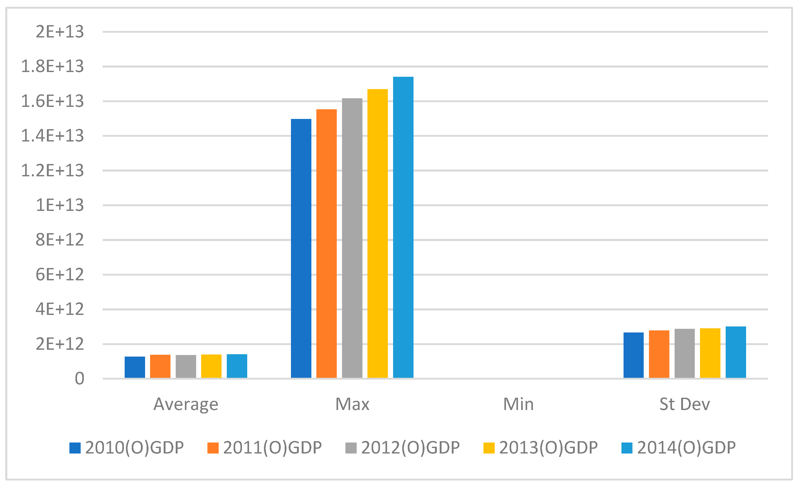
4.2. Statistical Analysis
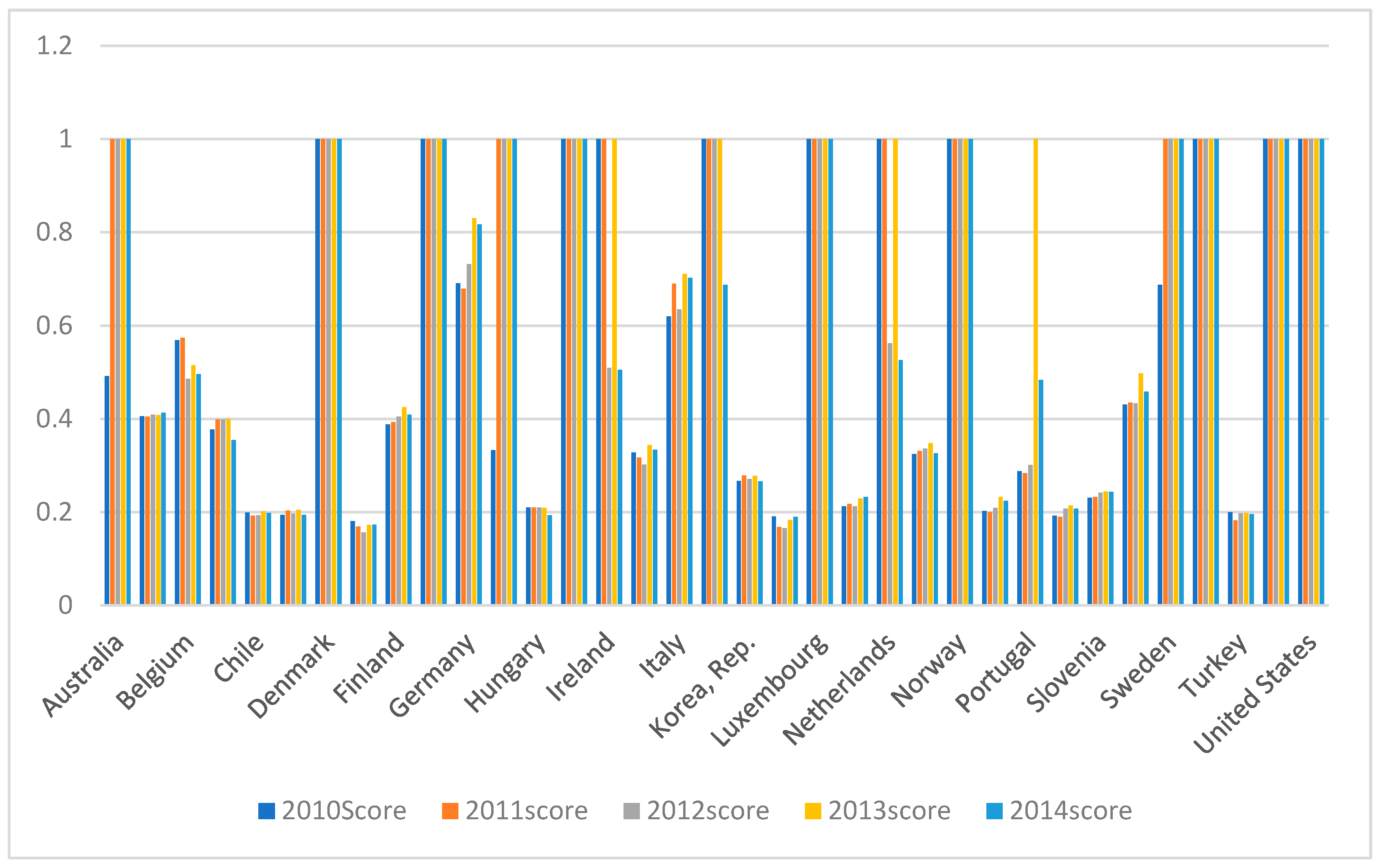
4.3. Overall Efficiency and Efficiencies in Each Year
4.4. Input and Output Efficiency
5. Conclusions and Policy Suggestions
- (1)
- There was a significant difference in the overall efficiencies in the OECD countries. Only Australia, Denmark, France, Iceland, Luxembourg, Norway, Switzerland, United Kingdom, and United States had overall efficiencies of 1 for the five years.
- (2)
- However, Chile, the Czech Republic, Estonia, Hungary, Latvia, Mexico, Poland, Slovak Republic, and Turkey all had efficiencies around or below 0.2 for the five years, and therefore, had a significant need for improvement. As the efficiencies in the other 16 countries ranged from 0.2 to 0.8, there was some room for improvement.
- (3)
- Germany, Italy, Sweden, and Australia had rising efficiencies and Belgium, Canada, Ireland, the Netherlands, and Japan had falling efficiencies. The Netherlands had a significant decline in 2012 and 2014, and efficiencies of 1 in all other years. Japan’s efficiency dropped in 2014, but was 1 in all other years.
- (4)
- The differences in traditional energy efficiencies between the countries was large. Australia, Demark, France, Iceland, Luxembourg, Norway, UK and USA all had traditional energy efficiencies 1; however, Austria, Belgium, Canada, Chile, Czech Republic, France, Hungary, Israel, Korea Republic, Latvia, Mexico, New Zealand, Poland, Slovak Republic, Slovenia, and Turkey only had efficiencies below 0.2 for the five consecutive years. Obviously, there is a significant need for traditional energy efficiency improvements in many countries. Eleven countries have new energy efficiencies of 1, which was more than the countries with traditional energy efficiencies of 1. However, Austria, Canada, Chile, Czech Republic, Latvia, Estonia, Finland, Germany, Hungary, Israel, Italy, New Zealand, Slovak, Slovenia, and Turkey all had new energy efficiencies of less than 0.2 and had a significant need for improvements. Most Eastern European countries (Cezch, Hungary, Latvia, Poland, Lovenia etc..) had new energy efficiency scores below 0.10, and there was still much room for improvement.
- (5)
- Belgium, Canada, Denmark, France, Germany, Iceland, Italy, Japan, Luxemburg, Netherlands, New Zealand, Spain, Sweden, Switzerland, United Kingdom, United States all had CO2 efficiencies of 1, and as the efficiencies in the other 19 countries were lower than 1, there was some need for improvement. Countries with relatively low carbon emission efficiency score were mainly Eastern European countries, Estonia only had an efficiency of 0.2 for the five years, while most other countries had efficiencies above 0.5.
- (6)
- The PM2.5 efficiencies were generally much lower than the CO2 efficiencies, with only eight countries; Denmark, France, Iceland, Luxembourg, Norway, Switzerland, United Kingdom, and the United States; having efficiencies of 1 for the five years compared to 16 countries with CO2 efficiencies of 1. Austria, Belgium, Canada, Chile, Czech Republic, Hungary, Israel, Korea Republic, Latvia, Mexico, New Zealand, Poland, Slovenia, and Turkey all had PM2.5 efficiencies below 0.2, with most being lower that 0.1; therefore, there was a significant need for improvement. It could also be seen that the efficiency score for most Eastern European countries was also below 0.1. There was a lot of room for improvement.
- (7)
- Countries that had poor traditional energy and new energy performances also had poor CO2 and PM2.5 performances.
- (8)
- Although the new energy performance in many countries still needs to be strengthened, new energy has been performing better with many of the OECD countries moving towards the sustainable development of new energy.
- Strengthening the development of new energy. The main new energy sources in Poland include offshore wind energy, nuclear energy and hydrogen energy. The development of new energy has become a top priority.
- Industrial restructuring. Most of the economic growth in Eastern European countries depends on coal-based oil-based manufacturing, which brings large environmental pollution. The adjustment of industrial structure requires long-term government planning to reduce emissions of environmental pollutants.
- Western Europe and Northern Europe have advanced technology and experience in environmental protection. International organizations should encourage developed countries provide technical assistance to Eastern European countries.
- The Belt and Road Initiative provides conditions for cooperation between China and Eastern European countries. Use China’s air pollution control experience to strengthen China’s cooperation with these Eastern European countries.
Author Contributions
Funding
Conflicts of Interest
References
- Bampatsou, C.; Papadopoulos, S.; Efthimios, Z. Technical efficiency of economic systems of EU-15 countries based on energy consumption. Energy Policy 2013, 55, 426–434. [Google Scholar] [CrossRef]
- Komiyama, R.; Fujii, Y. Assessment of massive integration of photovoltaic system considering Rechargeable Battery in Japan with High Time-Resolution Optimal Power Generation Mix Model. Energy Policy 2014, 66, 73–89. [Google Scholar] [CrossRef]
- Pang, R.H.; Deng, Z.Q.; Hu, J.L. Clean energy use and total-factor efficiencies: An international comparison. Renew. Sust. Energ. Rev. 2015, 52, 1158–1171. [Google Scholar] [CrossRef]
- Adewuyi, A.; Olabanji, B. Renewable and non-renewable energy-growth-emissions linkages: Review of emerging trends with policy implications. Renew. Sust. Energ Rev. 2017, 69, 275–291. [Google Scholar] [CrossRef]
- Jebali, E.; Essid, H.; Khraief, N. The analysis of energy efficiency of the Mediterranean countries: A two-stage double bootstrap DEA approach. Energy 2017, 134, 991–1000. [Google Scholar] [CrossRef]
- Atems, B.; Hotaling, C. The effect of renewable and nonrenewable electricity generation on economic growth. Energy Policy 2018, 112, 111–118. [Google Scholar] [CrossRef]
- Hoang, V.N.; Rao, D.S. Prasada Measuring and decomposing sustainable efficiency in agricultural production: A cumulative exergy balance approach. Ecol. Econ. 2010, 69, 1765–1776. [Google Scholar] [CrossRef]
- Shiau, T.A.; Jhang, J.S. An integration model of DEA and RST for measuring transport sustainability. Int. J. Sust. Dev. World 2010, 17, 76–83. [Google Scholar] [CrossRef]
- Camioto, F.d.C.; Mariano, E.B.; Rebelatto, D. Efficiency in Brazil’s industrial sectors in terms of energy and sustainable development. Environ. Sci. Policy 2014, 37, 50–60. [Google Scholar] [CrossRef]
- Wang, H. A generalized MCDA-DEA (multi-criterion decision analysis-data envelopment analysis) approach to construct slacks-based composite indicator. Energy 2015, 80, 114–122. [Google Scholar] [CrossRef]
- Zhang, N.; Xie, H. Toward green IT: Modeling sustainable production characteristics for Chinese electronic information industry, 1980–2012. Technol. Forecast Soc. Change 2015, 96, 62–70. [Google Scholar] [CrossRef]
- Raheli, H.; Rezaei, R.M.; Jadidi, M.R.; Mobtaker, H.G. A two-stage DEA model to evaluate sustainability and energy efficiency of tomato production. IPA 2017, 4, 342–350. [Google Scholar] [CrossRef]
- Chien, T.; Hu, J.L. Renewable energy and macroeconomic efficiency of OECD and non-OECD economies. Energy Policy 2007, 35, 3606–3615. [Google Scholar] [CrossRef]
- Honma, S.; Hu, J.L. Total-factor energy efficiency of regions in Japan. Energy Policy 2008, 36, 821–833. [Google Scholar] [CrossRef]
- Sueyoshi, T.; Goto, M. Should the US clean air act include CO2 emission control?: Examination by data nvelopment analysis. Energy Policy 2010, 38, 5902–5911. [Google Scholar] [CrossRef]
- Blokhuis, E.; Advokaat, B.; Schaefer, W. Assessing the performance of Dutch local energy companies. Energy Policy 2012, 45, 680–690. [Google Scholar] [CrossRef]
- Boubaker, K. A review on renewable energy conceptual perspectives in North Africa using a polynomial optimization scheme. Renev. Sust. Energ. Rev. 2012, 16, 4298–4302. [Google Scholar] [CrossRef]
- Fagiani, R.; Barquin, J.; Hakvoort, R. Risk-based assessment of the cost-efficiency and the effectivity of renewable energy support schemes: Certificate markets versus feed-in tariffs. Energy Policy 2013, 55, 648–661. [Google Scholar] [CrossRef]
- Menegaki, A.N.; Gurluk, S. Greece and Turkey: Assessment and comparison of their renewable energy performance. IJEEP 2013, 3, 367–383. [Google Scholar]
- Sueyoshi, T.; Goto, M. DEA environmental assessment in a time horizon: Malmquist index on fuel mix, electricity and CO2 of industrial nations. Energy Econ. 2013, 40, 370–382. [Google Scholar] [CrossRef]
- Azlina, A.A.; Law, S.H.; Mustapha, N.H.N. Dynamic linkages among transport energy consumption, income and CO2 emission in Malaysia. Energy Policy 2014, 73, 598–606. [Google Scholar] [CrossRef]
- Sueyoshi, T.; Goto, M. Photovoltaic Power stations in Germany and the United States: A comparative study by data envelopment analysis. Energy Econ. 2014, 42, 271–288. [Google Scholar] [CrossRef]
- Hampf, B.; Rodseth, K.L. Carbon dioxide emission standards for U.S. power plants: An efficiency analysis perspective. Energy Econ. 2015, 50, 140–153. [Google Scholar] [CrossRef]
- Kim, K.T.; Lee, D.J.; Park, S.J.; Zhang, Y.; Sultanov, A. Measuring the efficiency of the investment for renewable energy in Korea using data envelopment analysis. Renew. Sust. Energ. Rev. 2015, 47, 694–702. [Google Scholar] [CrossRef]
- Sueyoshi, T.; Goto, M. Japanese fuel mix strategy after disaster of Fukushima Daiichi nuclear power plant: lessons from international comparison among industrial nations measured by DEA environmental assessment in time horizon. Energy Econ. 2015, 52, 87–103. [Google Scholar] [CrossRef]
- Wu, J.; Lv, L.; Sun, J. A comprehensive analysis of China’s regional energy saving and emission reduction efficiency: From production and treatment perspectives. Energy Policy 2015, 84, 166–176. [Google Scholar] [CrossRef]
- Lin, B.; Li, J. Does China’s energy development plan affect energy conservation? Empirical evidence from coal-fired power generation. Emerg. Mark. Financ. Tr. 2015, 51, 798–811. [Google Scholar] [CrossRef]
- Ervural, B.C.; Bilal, E.; Zaim, S. Energy efficiency evaluation of provinces in Turkey using data envelopment analysis. Procedia Soc. Behav. Sci. 2016, 235, 139–148. [Google Scholar] [CrossRef]
- Guo, X.; Lu, C.C.; Lee, J.H.; Chiu, Y.H. Applying the dynamic DEA model to evaluate the energy efficiency of OECD countries and China. Energy 2017, 134, 392–399. [Google Scholar] [CrossRef]
- Mehmeti, A.; McPhail, S.; Ulgiati, S. Fuel cell eco-efficiency calculator (FCEC): A simulation tool for the environmental and economic performance of high-temperature fuel cells. Energy 2018, 159, 1195–1205. [Google Scholar] [CrossRef]
- Steinberg, D.C.; Bielen, D.A.; Townsend, A. Evaluating the CO2 emissions reduction potential and cost of power sector re-dispatch. Energy Policy 2018, 112, 33–34. [Google Scholar] [CrossRef]
- Llamas, T.; Armando, R.; Probst, O. On the role of efficient cogeneration for meeting Mexico’s clean energy goals. Energy Policy 2018, 112, 173–183. [Google Scholar] [CrossRef]
- Farrell, M.J. The Measurement of Productive Efficiency. J. R. Stat. Soc. 1957, 120, 253–281. [Google Scholar] [CrossRef]
- Charnes, A.; Cooper, W.; Rhodes, E. Measuring the efficiency of decision-making units. Eur. J. Oper. Res. 1978, 2, 429–444. [Google Scholar] [CrossRef]
- Banker, R.D.; Charnes, R.F.; Cooper, W.W. Some models for estimating technical and scale inefficiencies in data envelopment analysis. Manag. Sci. 1984, 30, 1078–1092. [Google Scholar] [CrossRef]
- Tone‚, K. A slacks-based measure of efficiency in data envelopment analysis. Eur. J. Oper. Res 2001, 130, 498–509. [Google Scholar]
- Klopp, G.A. The analysis of the efficiency of production system with multiple inputs and outputs. Ph.D. Thesis, Industrial and System Engineering College, University of Illinois, Chicago, IL, USA, 1985. [Google Scholar]
- Malmquist, S. Index numbers and indifference surfaces. Trabajos de Estadistica 1953, 4, 209–242. [Google Scholar] [CrossRef]
- Färe, R.; Grosskopf, S.; Norris, M.; Zhang, Z. Productivity growth technical progress and efficiency change in industrialized countries. Am. Econ. Rev. 1994, 84, 66–83. [Google Scholar]
- Färe, R.; Grosskopf, S. Productivity and intermediate products: A frontier approach. Econ. Lett. 1996, 50, 65–70. [Google Scholar] [CrossRef]
- Bogetoft, P.; Christensen, D.L.; Damgard, I.; Geisler, M.; Jakobsen, T.P.; Krøigaard, M.; Nielsen, J.D.; Nielsen, J.B.; Nielsen, K.; Pagter, J.; Schwartzbach, M.I.; Toft, T. Secure Multiparty Computation Goes Live. In Financial Cryptography and Data Security, Proceedings of the 18th International Conference on Financial Cryptography and Data Security, Barbados, USA, 3–7 March 2014; Springer: Berlin/Heidelberg, Germany, 2008; Volume 5628, pp. 325–343. [Google Scholar]
- Chen, C.M. Network-DEA, A Model with New Efficiency Measures to Incorporate the Dynamic Effect in Production Networks. Eur. J Oper. Res. 2009, 194, 687–699. [Google Scholar] [CrossRef]
- Nemoto, J.; Goto, M. Dynamic data envelopment analysis: modeling intertemporal behavior of a firm in the presence of productive inefficiencies. Econ. Lett. 1999, 64, 51–56. [Google Scholar] [CrossRef]
- Park, K.S.; Park, K. Measurement of multiperiod aggregative efficiency. Eur. J Oper Res. 2009, 193, 567–580. [Google Scholar] [CrossRef]
- Chang, H.; Choy, H.L.; Cooper, W.W.; Ruefli, T.W. Using Malmquist indexes to measure changes in the productivity and efficiency of US accounting firms before and after the Sarbanes-Oxley. Act. Omega 2009, 37, 951–960. [Google Scholar] [CrossRef]
- Sueyoshi, T.; Sekitani, K. Returns to scale in dynamic DEA. Eur. J. Oper Res 2005, 161, 536–544. [Google Scholar] [CrossRef]
- Tone, K.; Tsutsui, M. Dynamic DEA: A Slacks-based measure approach. Omega 2010, 38, 145–156. [Google Scholar] [CrossRef]
- Hu, J.L.; Wang, S.C. Total-factor energy efficiency of regions in China. Energy Policy 2006, 34, 3206–3217. [Google Scholar] [CrossRef]
- World Development Indicators of World Bank. 2017. Available online: https:// data. worldbank. org/indicator (accessed on 9 April 2018).


| Input Variables | Desirable Output Variables | Undesirable Output Variables | Carry-Over |
|---|---|---|---|
| Labor (Lab) | GDP | CO2 | Fixed assets (asset) |
| Energy consumption | PM2.5 | ||
| New energy consumption |
| NO. | DMU | Total | 2010 | 2011 | 2012 | 2013 | 2014 |
|---|---|---|---|---|---|---|---|
| 1 | Australia | 0.8830 | 0.4921 | 1.0000 | 1.0000 | 1.0000 | 1.0000 |
| 2 | Austria | 0.4079 | 0.4058 | 0.4043 | 0.4088 | 0.4077 | 0.4127 |
| 3 | Belgium | 0.5277 | 0.5690 | 0.5741 | 0.4860 | 0.5149 | 0.4957 |
| 4 | Canada | 0.3858 | 0.3773 | 0.3991 | 0.3989 | 0.4004 | 0.3543 |
| 5 | Chile | 0.1966 | 0.1987 | 0.1923 | 0.1931 | 0.2011 | 0.1977 |
| 6 | Czech Republic | 0.1986 | 0.1941 | 0.2032 | 0.1967 | 0.2051 | 0.1939 |
| 7 | Denmark | 1.0000 | 1.0000 | 1.0000 | 1.0000 | 1.0000 | 1.0000 |
| 8 | Estonia | 0.1703 | 0.1802 | 0.1690 | 0.1565 | 0.1724 | 0.1732 |
| 9 | Finland | 0.4038 | 0.3877 | 0.3928 | 0.4044 | 0.4245 | 0.4093 |
| 10 | France | 1.0000 | 1.0000 | 1.0000 | 1.0000 | 1.0000 | 1.0000 |
| 11 | Germany | 0.7480 | 0.6907 | 0.6792 | 0.7316 | 0.8299 | 0.8167 |
| 12 | Greece | 0.8285 | 0.3329 | 1.0000 | 1.0000 | 1.0000 | 1.0000 |
| 13 | Hungary | 0.2062 | 0.2098 | 0.2097 | 0.2095 | 0.2087 | 0.1932 |
| 14 | Iceland | 1.0000 | 1.0000 | 1.0000 | 1.0000 | 1.0000 | 1.0000 |
| 15 | Ireland | 0.7665 | 1.0000 | 1.0000 | 0.5094 | 1.0000 | 0.5054 |
| 16 | Israel | 0.3245 | 0.3274 | 0.3165 | 0.3019 | 0.3433 | 0.3339 |
| 17 | Italy | 0.6712 | 0.6193 | 0.6898 | 0.6346 | 0.7107 | 0.7027 |
| 18 | Japan | 0.9313 | 1.0000 | 1.0000 | 1.0000 | 1.0000 | 0.6879 |
| 19 | Korea, Rep. | 0.2718 | 0.2666 | 0.2780 | 0.2711 | 0.2779 | 0.2655 |
| 20 | Latvia | 0.1795 | 0.1907 | 0.1678 | 0.1658 | 0.1829 | 0.1901 |
| 21 | Luxembourg | 1.0000 | 1.0000 | 1.0000 | 1.0000 | 1.0000 | 1.0000 |
| 22 | Mexico | 0.2208 | 0.2119 | 0.2172 | 0.2126 | 0.2293 | 0.2327 |
| 23 | Netherlands | 0.7914 | 1.0000 | 1.0000 | 0.5618 | 1.0000 | 0.5258 |
| 24 | New Zealand | 0.3330 | 0.3243 | 0.3314 | 0.3358 | 0.3481 | 0.3257 |
| 25 | Norway | 1.0000 | 1.0000 | 1.0000 | 1.0000 | 1.0000 | 1.0000 |
| 26 | Poland | 0.2136 | 0.2019 | 0.2002 | 0.2091 | 0.2328 | 0.2237 |
| 27 | Portugal | 0.4404 | 0.2877 | 0.2834 | 0.3008 | 1.0000 | 0.4834 |
| 28 | Slovak Republic | 0.2020 | 0.1925 | 0.1896 | 0.2069 | 0.2142 | 0.2070 |
| 29 | Slovenia | 0.2382 | 0.2306 | 0.2322 | 0.2413 | 0.2440 | 0.2428 |
| 30 | Spain | 0.4502 | 0.4304 | 0.4350 | 0.4328 | 0.4973 | 0.4578 |
| 31 | Sweden | 0.9364 | 0.6874 | 1.0000 | 1.0000 | 1.0000 | 1.0000 |
| 32 | Switzerland | 1.0000 | 1.0000 | 1.0000 | 1.0000 | 1.0000 | 1.0000 |
| 33 | Turkey | 0.1946 | 0.1997 | 0.1825 | 0.1973 | 0.1985 | 0.1953 |
| 34 | United Kingdom | 1.0000 | 1.0000 | 1.0000 | 1.0000 | 1.0000 | 1.0000 |
| 35 | United States | 1.0000 | 1.0000 | 1.0000 | 1.0000 | 1.0000 | 1.0000 |
| DMU | 2010 Labor | 2011 Labor | 2012 Labor | 2013 Labor | 2014 Labor |
|---|---|---|---|---|---|
| Australia | 1.0000 | 1.0000 | 1.0000 | 1.0000 | 1.0000 |
| Austria | 1.0000 | 1.0000 | 1.0000 | 1.0000 | 1.0000 |
| Belgium | 1.0000 | 1.0000 | 1.0000 | 1.0000 | 1.0000 |
| Canada | 0.9144 | 0.9655 | 0.9493 | 0.9173 | 0.8416 |
| Chile | 0.3580 | 0.3745 | 0.3897 | 0.3926 | 0.3312 |
| Czech Republic | 0.4154 | 0.4411 | 0.4811 | 0.4718 | 0.4281 |
| Denmark | 1.0000 | 1.0000 | 1.0000 | 1.0000 | 1.0000 |
| Estonia | 0.3737 | 0.4140 | 0.4114 | 0.4426 | 0.4253 |
| Finland | 1.0000 | 1.0000 | 1.0000 | 1.0000 | 1.0000 |
| France | 1.0000 | 1.0000 | 1.0000 | 1.0000 | 1.0000 |
| Germany | 0.9678 | 0.9836 | 0.9429 | 0.9527 | 0.9426 |
| Greece | 0.7625 | 1.0000 | 1.0000 | 1.0000 | 1.0000 |
| Hungary | 0.3993 | 0.4008 | 0.3578 | 0.3684 | 0.3395 |
| Iceland | 1.0000 | 1.0000 | 1.0000 | 1.0000 | 1.0000 |
| Ireland | 1.0000 | 1.0000 | 1.0000 | 1.0000 | 1.0000 |
| Israel | 0.8765 | 0.9074 | 0.8638 | 0.9444 | 0.8886 |
| Italy | 1.0000 | 1.0000 | 0.9768 | 1.0000 | 0.9407 |
| Japan | 1.0000 | 1.0000 | 1.0000 | 1.0000 | 0.7143 |
| Korea, Rep. | 0.4546 | 0.4745 | 0.4603 | 0.4714 | 0.4782 |
| Latvia | 0.2931 | 0.3346 | 0.3300 | 0.3559 | 0.3420 |
| Luxembourg | 1.0000 | 1.0000 | 1.0000 | 1.0000 | 1.0000 |
| Mexico | 0.2182 | 0.2294 | 0.2180 | 0.2214 | 0.2175 |
| Netherlands | 1.0000 | 1.0000 | 1.0000 | 1.0000 | 1.0000 |
| New Zealand | 0.8269 | 0.8796 | 0.9117 | 0.9542 | 0.8928 |
| Norway | 1.0000 | 1.0000 | 1.0000 | 1.0000 | 1.0000 |
| Poland | 0.2788 | 0.2957 | 0.2691 | 0.2896 | 0.2723 |
| Portugal | 0.5004 | 0.5541 | 0.4955 | 1.0000 | 0.6299 |
| Slovak Republic | 0.4374 | 0.4492 | 0.4213 | 0.4345 | 0.4065 |
| Slovenia | 0.6037 | 0.6167 | 0.5574 | 0.5701 | 0.5384 |
| Spain | 0.7045 | 0.6780 | 0.6291 | 0.6546 | 0.6322 |
| Sweden | 0.9692 | 1.0000 | 1.0000 | 1.0000 | 1.0000 |
| Switzerland | 1.0000 | 1.0000 | 1.0000 | 1.0000 | 1.0000 |
| Turkey | 0.3212 | 0.3209 | 0.3203 | 0.3257 | 0.2997 |
| United Kingdom | 1.0000 | 1.0000 | 1.0000 | 1.0000 | 1.0000 |
| United States | 1.0000 | 1.0000 | 1.0000 | 1.0000 | 1.0000 |
| DMU | 2010 Asset | 2011 Asset | 2012 Asset | 2013 Asset | 2014 Asset |
|---|---|---|---|---|---|
| Australia | 0.6857 | 1.0000 | 1.0000 | 1.0000 | 1.0000 |
| Austria | 0.9801 | 0.9812 | 0.9573 | 0.9413 | 0.9721 |
| Belgium | 0.9090 | 0.9287 | 1.0000 | 1.0000 | 0.9333 |
| Canada | 0.8047 | 0.8065 | 0.8134 | 0.8067 | 0.8205 |
| Chile | 0.6776 | 0.6314 | 0.5958 | 0.6383 | 0.7365 |
| Czech Republic | 0.6782 | 0.6879 | 0.6018 | 0.6632 | 0.6611 |
| Denmark | 1.0000 | 1.0000 | 1.0000 | 1.0000 | 1.0000 |
| Estonia | 0.7370 | 0.6197 | 0.5417 | 0.6079 | 0.6313 |
| Finland | 0.9296 | 1.0000 | 0.9555 | 1.0000 | 0.8922 |
| France | 1.0000 | 1.0000 | 1.0000 | 1.0000 | 1.0000 |
| Germany | 1.0000 | 1.0000 | 1.0000 | 1.0000 | 1.0000 |
| Greece | 0.9197 | 1.0000 | 1.0000 | 1.0000 | 1.0000 |
| Hungary | 0.7589 | 0.7606 | 0.8100 | 0.7772 | 0.7338 |
| Iceland | 1.0000 | 1.0000 | 1.0000 | 1.0000 | 1.0000 |
| Ireland | 1.0000 | 1.0000 | 1.0000 | 1.0000 | 1.0000 |
| Israel | 0.8502 | 0.7627 | 0.7420 | 0.8196 | 0.8468 |
| Italy | 1.0000 | 1.0000 | 1.0000 | 1.0000 | 1.0000 |
| Japan | 1.0000 | 1.0000 | 1.0000 | 1.0000 | 0.8044 |
| Korea, Rep. | 0.5744 | 0.5627 | 0.6242 | 0.6791 | 0.6894 |
| Latvia | 0.8116 | 0.6181 | 0.6020 | 0.6694 | 0.7478 |
| Luxembourg | 1.0000 | 1.0000 | 1.0000 | 1.0000 | 1.0000 |
| Mexico | 0.8340 | 0.8331 | 0.8395 | 0.9122 | 0.9344 |
| Netherlands | 1.0000 | 1.0000 | 1.0000 | 1.0000 | 1.0000 |
| New Zealand | 0.7808 | 0.7611 | 0.7531 | 0.7421 | 0.7576 |
| Norway | 1.0000 | 1.0000 | 1.0000 | 1.0000 | 1.0000 |
| Poland | 0.8631 | 0.8264 | 0.9219 | 1.0000 | 0.9911 |
| Portugal | 1.0000 | 0.8366 | 1.0000 | 1.0000 | 1.0000 |
| Slovak Republic | 0.6529 | 0.6232 | 0.7527 | 0.7796 | 0.7783 |
| Slovenia | 0.7050 | 0.7164 | 0.8424 | 0.8395 | 0.8737 |
| Spain | 0.9103 | 1.0000 | 1.0000 | 1.0000 | 0.9097 |
| Sweden | 0.9907 | 1.0000 | 1.0000 | 1.0000 | 1.0000 |
| Switzerland | 1.0000 | 1.0000 | 1.0000 | 1.0000 | 1.0000 |
| Turkey | 0.6820 | 1.0000 | 0.6837 | 0.6638 | 0.6952 |
| United Kingdom | 1.0000 | 1.0000 | 1.0000 | 1.0000 | 1.0000 |
| United States | 1.0000 | 1.0000 | 1.0000 | 1.0000 | 1.0000 |
| No. | DMU | 2010 Energy | 2011 Energy | 2012 Energy | 2013 Energy | 2014 Energy |
|---|---|---|---|---|---|---|
| 1 | Australia | 0.1595 | 1.0000 | 1.0000 | 1.0000 | 1.0000 |
| 2 | Austria | 0.1442 | 0.1443 | 0.1590 | 0.1642 | 0.1677 |
| 3 | Belgium | 0.1812 | 0.2036 | 0.1827 | 0.1853 | 0.1489 |
| 4 | Canada | 0.1549 | 0.1898 | 0.1960 | 0.1714 | 0.1200 |
| 5 | Chile | 0.1016 | 0.1074 | 0.1219 | 0.1242 | 0.0972 |
| 6 | Czech Republic | 0.0147 | 0.0156 | 0.0864 | 0.0853 | 0.0761 |
| 7 | Denmark | 1.0000 | 1.0000 | 1.0000 | 1.0000 | 1.0000 |
| 8 | Estonia | 0.0342 | 0.0401 | 0.0376 | 0.0448 | 0.0495 |
| 9 | Finland | 0.0663 | 0.1423 | 0.0955 | 0.2169 | 0.2460 |
| 10 | France | 1.0000 | 1.0000 | 1.0000 | 1.0000 | 1.0000 |
| 11 | Germany | 0.7938 | 0.7861 | 0.8961 | 0.7934 | 0.8350 |
| 12 | Greece | 0.1195 | 1.0000 | 1.0000 | 1.0000 | 1.0000 |
| 13 | Hungary | 0.0636 | 0.0627 | 0.0571 | 0.0601 | 0.0563 |
| 14 | Iceland | 1.0000 | 1.0000 | 1.0000 | 1.0000 | 1.0000 |
| 15 | Ireland | 1.0000 | 1.0000 | 0.1349 | 1.0000 | 0.1428 |
| 16 | Israel | 0.0875 | 0.0885 | 0.0851 | 0.0927 | 0.0874 |
| 17 | Italy | 0.4500 | 0.5232 | 0.6819 | 0.8137 | 0.8859 |
| 18 | Japan | 1.0000 | 1.0000 | 1.0000 | 1.0000 | 0.6103 |
| 19 | Korea, Rep. | 0.0743 | 0.0784 | 0.0759 | 0.0771 | 0.0817 |
| 20 | Latvia | 0.0130 | 0.0146 | 0.0155 | 0.0158 | 0.0151 |
| 21 | Luxembourg | 1.0000 | 1.0000 | 1.0000 | 1.0000 | 1.0000 |
| 22 | Mexico | 0.0653 | 0.0698 | 0.0673 | 0.0692 | 0.0686 |
| 23 | Netherlands | 1.0000 | 1.0000 | 0.2224 | 1.0000 | 0.2040 |
| 24 | New Zealand | 0.0865 | 0.0920 | 0.0904 | 0.0958 | 0.0916 |
| 25 | Norway | 1.0000 | 1.0000 | 1.0000 | 1.0000 | 1.0000 |
| 26 | Poland | 0.0292 | 0.0310 | 0.0284 | 0.0624 | 0.0289 |
| 27 | Portugal | 0.0670 | 0.1056 | 0.1045 | 1.0000 | 0.4553 |
| 28 | Slovak Republic | 0.0460 | 0.0468 | 0.0447 | 0.0454 | 0.0432 |
| 29 | Slovenia | 0.0260 | 0.0258 | 0.0228 | 0.0231 | 0.0229 |
| 30 | Spain | 0.2872 | 0.3083 | 0.3654 | 0.4239 | 0.4436 |
| 31 | Sweden | 0.6647 | 1.0000 | 1.0000 | 1.0000 | 1.0000 |
| 32 | Switzerland | 1.0000 | 1.0000 | 1.0000 | 1.0000 | 1.0000 |
| 33 | Turkey | 0.0487 | 0.0499 | 0.0505 | 0.0535 | 0.0497 |
| 34 | United Kingdom | 1.0000 | 1.0000 | 1.0000 | 1.0000 | 1.0000 |
| 35 | United States | 1.0000 | 1.0000 | 1.0000 | 1.0000 | 1.0000 |
| No. | DMU | 2011 New Energy | 2012 New Energy | 2013 New Energy | 2014 New Energy |
|---|---|---|---|---|---|
| 1 | Australia | 1.0000 | 1.0000 | 1.0000 | 1.0000 |
| 2 | Austria | 0.0942 | 0.1054 | 0.1080 | 0.1132 |
| 3 | Belgium | 0.7831 | 0.3314 | 0.4552 | 0.4511 |
| 4 | Canada | 0.0467 | 0.0460 | 0.0935 | 0.0448 |
| 5 | Chile | 0.0150 | 0.0160 | 0.0199 | 0.0238 |
| 6 | Czech Republic | 0.0114 | 0.0337 | 0.0370 | 0.0393 |
| 7 | Denmark | 1.0000 | 1.0000 | 1.0000 | 1.0000 |
| 8 | Estonia | 0.0016 | 0.0017 | 0.0022 | 0.0025 |
| 9 | Finland | 0.0590 | 0.0294 | 0.0814 | 0.0682 |
| 10 | France | 1.0000 | 1.0000 | 1.0000 | 1.0000 |
| 11 | Germany | 0.2928 | 0.3352 | 0.7563 | 0.6759 |
| 12 | Greece | 1.0000 | 1.0000 | 1.0000 | 1.0000 |
| 13 | Hungary | 0.0249 | 0.0228 | 0.0285 | 0.0326 |
| 14 | Iceland | 1.0000 | 1.0000 | 1.0000 | 1.0000 |
| 15 | Ireland | 1.0000 | 0.5928 | 1.0000 | 0.6183 |
| 16 | Israel | 0.0496 | 0.0538 | 0.0662 | 0.0797 |
| 17 | Italy | 0.6014 | 0.2480 | 0.3997 | 0.4270 |
| 18 | Japan | 1.0000 | 1.0000 | 1.0000 | 0.9778 |
| 19 | Korea, Rep. | 0.4695 | 0.3977 | 0.3633 | 0.2548 |
| 20 | Latvia | 0.0014 | 0.0013 | 0.0016 | 0.0019 |
| 21 | Luxembourg | 1.0000 | 1.0000 | 1.0000 | 1.0000 |
| 22 | Mexico | 0.0680 | 0.0695 | 0.0731 | 0.0679 |
| 23 | Netherlands | 1.0000 | 0.6113 | 1.0000 | 0.4596 |
| 24 | New Zealand | 0.0090 | 0.0104 | 0.0135 | 0.0157 |
| 25 | Norway | 1.0000 | 1.0000 | 1.0000 | 1.0000 |
| 26 | Poland | 0.0266 | 0.0240 | 0.0417 | 0.0242 |
| 27 | Portugal | 0.0154 | 0.0218 | 1.0000 | 0.1895 |
| 28 | Slovak Republic | 0.0162 | 0.0162 | 0.0199 | 0.0201 |
| 29 | Slovenia | 0.0047 | 0.0042 | 0.0047 | 0.0053 |
| 30 | Spain | 0.1231 | 0.0932 | 0.2181 | 0.1628 |
| 31 | Sweden | 1.0000 | 1.0000 | 1.0000 | 1.0000 |
| 32 | Switzerland | 1.0000 | 1.0000 | 1.0000 | 1.0000 |
| 33 | Turkey | 0.0342 | 0.0357 | 0.0367 | 0.0413 |
| 34 | United Kingdom | 1.0000 | 1.0000 | 1.0000 | 1.0000 |
| 35 | United States | 1.0000 | 1.0000 | 1.0000 | 1.0000 |
| No. | DMU | 2010 CO2 | 2011 CO2 | 2012 CO2 | 2013 CO2 | 2014 CO2 |
|---|---|---|---|---|---|---|
| 1 | Australia | 0.9758 | 1.0000 | 1.0000 | 1.0000 | 1.0000 |
| 2 | Austria | 0.7353 | 0.7215 | 0.7563 | 0.7616 | 0.7328 |
| 3 | Belgium | 1.0000 | 1.0000 | 1.0000 | 1.0000 | 1.0000 |
| 4 | Canada | 1.0000 | 1.0000 | 1.0000 | 1.0000 | 1.0000 |
| 5 | Chile | 0.6111 | 0.5442 | 0.5807 | 0.5595 | 0.4390 |
| 6 | Czech Republic | 0.6704 | 0.7268 | 0.3613 | 0.3549 | 0.2992 |
| 7 | Denmark | 1.0000 | 1.0000 | 1.0000 | 1.0000 | 1.0000 |
| 8 | Estonia | 0.2175 | 0.2129 | 0.2302 | 0.2113 | 0.1866 |
| 9 | Finland | 1.0000 | 0.5646 | 1.0000 | 0.6366 | 0.6681 |
| 10 | France | 1.0000 | 1.0000 | 1.0000 | 1.0000 | 1.0000 |
| 11 | Germany | 1.0000 | 1.0000 | 1.0000 | 1.0000 | 1.0000 |
| 12 | Greece | 0.7213 | 1.0000 | 1.0000 | 1.0000 | 1.0000 |
| 13 | Hungary | 0.5267 | 0.5030 | 0.5048 | 0.5367 | 0.4624 |
| 14 | Iceland | 1.0000 | 1.0000 | 1.0000 | 1.0000 | 1.0000 |
| 15 | Ireland | 1.0000 | 1.0000 | 0.7403 | 1.0000 | 0.5930 |
| 16 | Israel | 0.6852 | 0.6470 | 0.5996 | 0.7294 | 0.6630 |
| 17 | Italy | 1.0000 | 1.0000 | 1.0000 | 1.0000 | 0.9472 |
| 18 | Japan | 1.0000 | 1.0000 | 1.0000 | 1.0000 | 1.0000 |
| 19 | Korea, Rep. | 0.6963 | 0.6954 | 0.6636 | 0.6811 | 0.7261 |
| 20 | Latvia | 0.5944 | 0.6615 | 0.7008 | 0.7160 | 0.6256 |
| 21 | Luxembourg | 1.0000 | 1.0000 | 1.0000 | 1.0000 | 1.0000 |
| 22 | Mexico | 0.8163 | 0.8241 | 0.7576 | 0.7955 | 0.8167 |
| 23 | Netherlands | 1.0000 | 1.0000 | 1.0000 | 1.0000 | 1.0000 |
| 24 | New Zealand | 0.9318 | 0.9141 | 0.9081 | 0.9524 | 0.8041 |
| 25 | Norway | 1.0000 | 1.0000 | 1.0000 | 1.0000 | 1.0000 |
| 26 | Poland | 0.5464 | 0.5686 | 0.5286 | 0.4796 | 0.5763 |
| 27 | Portugal | 0.7056 | 0.8791 | 0.8375 | 1.0000 | 0.9650 |
| 28 | Slovak Republic | 0.4990 | 0.4861 | 0.5018 | 0.4978 | 0.4570 |
| 29 | Slovenia | 0.6326 | 0.5811 | 0.5520 | 0.5687 | 0.5410 |
| 30 | Spain | 1.0000 | 1.0000 | 1.0000 | 1.0000 | 1.0000 |
| 31 | Sweden | 1.0000 | 1.0000 | 1.0000 | 1.0000 | 1.0000 |
| 32 | Switzerland | 1.0000 | 1.0000 | 1.0000 | 1.0000 | 1.0000 |
| 33 | Turkey | 0.9339 | 0.8845 | 0.8404 | 0.9047 | 0.8157 |
| 34 | United Kingdom | 1.0000 | 1.0000 | 1.0000 | 1.0000 | 1.0000 |
| 35 | United States | 1.0000 | 1.0000 | 1.0000 | 1.0000 | 1.0000 |
| No. | DMU | 2010 PM2.5 | 2011 PM2.5 | 2012 PM2.5 | 2013 PM2.5 | 2014 PM2.5 |
|---|---|---|---|---|---|---|
| 1 | Australia | 0.4342 | 1.0000 | 1.0000 | 1.0000 | 1.0000 |
| 2 | Austria | 0.1572 | 0.1609 | 0.1675 | 0.1671 | 0.1725 |
| 3 | Belgium | 0.1706 | 0.1913 | 0.1200 | 0.1541 | 0.1668 |
| 4 | Canada | 0.1934 | 0.2259 | 0.2306 | 0.2742 | 0.1329 |
| 5 | Chile | 0.0508 | 0.0545 | 0.0574 | 0.0590 | 0.0506 |
| 6 | Czech Republic | 0.0059 | 0.0064 | 0.0513 | 0.0475 | 0.0413 |
| 7 | Denmark | 1.0000 | 1.0000 | 1.0000 | 1.0000 | 1.0000 |
| 8 | Estonia | 0.0118 | 0.0136 | 0.0150 | 0.0138 | 0.0123 |
| 9 | Finland | 0.0965 | 0.2318 | 0.1420 | 0.3026 | 0.2885 |
| 10 | France | 1.0000 | 1.0000 | 1.0000 | 1.0000 | 1.0000 |
| 11 | Germany | 0.6625 | 0.6183 | 0.7461 | 0.8348 | 0.8288 |
| 12 | Greece | 0.1273 | 1.0000 | 1.0000 | 1.0000 | 1.0000 |
| 13 | Hungary | 0.0284 | 0.0299 | 0.0285 | 0.0290 | 0.0261 |
| 14 | Iceland | 1.0000 | 1.0000 | 1.0000 | 1.0000 | 1.0000 |
| 15 | Ireland | 1.0000 | 1.0000 | 0.2437 | 1.0000 | 0.3099 |
| 16 | Israel | 0.0640 | 0.0678 | 0.0661 | 0.0692 | 0.0633 |
| 17 | Italy | 0.5044 | 0.6028 | 0.5647 | 0.6091 | 0.5802 |
| 18 | Japan | 1.0000 | 1.0000 | 1.0000 | 1.0000 | 0.6126 |
| 19 | Korea, Rep. | 0.0250 | 0.0281 | 0.0278 | 0.0256 | 0.0251 |
| 20 | Latvia | 0.0064 | 0.0073 | 0.0081 | 0.0074 | 0.0067 |
| 21 | Luxembourg | 1.0000 | 1.0000 | 1.0000 | 1.0000 | 1.0000 |
| 22 | Mexico | 0.0299 | 0.0318 | 0.0295 | 0.0311 | 0.0310 |
| 23 | Netherlands | 1.0000 | 1.0000 | 0.2172 | 1.0000 | 0.2007 |
| 24 | New Zealand | 0.1340 | 0.1438 | 0.1489 | 0.1567 | 0.1488 |
| 25 | Norway | 1.0000 | 1.0000 | 1.0000 | 1.0000 | 1.0000 |
| 26 | Poland | 0.0100 | 0.0109 | 0.0110 | 0.0302 | 0.0107 |
| 27 | Portugal | 0.1171 | 0.1208 | 0.1193 | 1.0000 | 0.5055 |
| 28 | Slovak Republic | 0.0218 | 0.0232 | 0.0229 | 0.0232 | 0.0209 |
| 29 | Slovenia | 0.0150 | 0.0156 | 0.0136 | 0.0125 | 0.0109 |
| 30 | Spain | 0.4021 | 0.3627 | 0.3824 | 0.5364 | 0.4809 |
| 31 | Sweden | 0.9334 | 1.0000 | 1.0000 | 1.0000 | 1.0000 |
| 32 | Switzerland | 1.0000 | 1.0000 | 1.0000 | 1.0000 | 1.0000 |
| 33 | Turkey | 0.0136 | 0.0144 | 0.0155 | 0.0147 | 0.0132 |
| 34 | United Kingdom | 1.0000 | 1.0000 | 1.0000 | 1.0000 | 1.0000 |
| 35 | United States | 1.0000 | 1.0000 | 1.0000 | 1.0000 | 1.0000 |
| No. | DMU | Energy | New Energy | CO2 | PM2.5 | |
|---|---|---|---|---|---|---|
| 1 | Australia | The first year was less than 0.2, the other years were 1. | 1 for 5 years | Last 4 years were 1 and the room for improvement was 0. | The room for improvement was 0. | |
| 2 | Austria | Below 0.2, but continued to rise | Continue to rise to around 0.1 | For more than five consecutive years, it was above 0.7, a slight decline in the last year | Slightly increased for five consecutive years, but all efficiency scores were below 0.2 | |
| 3 | Belgium | Fluctuated between 0.1 and 0.2 | From 0.8 in 2010 to around 0.3 Then rising to around 0.5 | 1 for 5 years | Five years below 0.2 and falling | |
| 4 | Canada | Fluctuated between 0.1 and 0.2 | Below 0.1 and decreasing | 1 for 5 years | Below 0.3, the previous four years rose but the last year dropped to around 0.1 | |
| 5 | Chile | Fluctuated around 0.1 | Less than 0.1, then slightly rise | From 0.6 in the first year, down to 0.4 in the last year | Below 0.1, the first four years rose, the last year fell slightly | |
| 6 | Czech Republic | From about 0 to about 0.1, and the last two years dropped slightly | Less than 0.1, then slightly rise | In 2010, 0.6 rose to 0.7 in 2011, and then fell to around 0.3. | Far below 0.1, and continued to decline | |
| 7 | Denmark | 1 for 5 years | 1 for 5 years | 1 for 5 years | 1 for 5 years | |
| 8 | Estonia | Less than 0.1, slightly rising | Close to 0 | Five years around 0.2 | Lower than 0.1 | |
| 9 | Finland | From 0.1 fluctuated to above 0.2 | Below 0.1 and declining | From 1 in 2010, down to 0.6 | From 0.2 in 2010 to 0.3 in 2014 | |
| 10 | France | 1 for 5 years | 1 for 5 years | 1 for 5 years | 1 for 5 years | |
| 11 | Germany | Fluctuating around 0.8 | Rose from around 0.3 in 2010 to nearly 0.8 in 2013, and dropped slightly to around 0.7 after 2014. | 1 for 5 years | From about 0.6 in 2010 to 0.8 | |
| 12 | Greece | In 2010, it was 0.1, and after four years, it was 1 | 1 for 5 years | In 2010 it was 0.7 and then rose to 1 | In 2010, it was about 0.1, and then rose to 1 in the last 4 years. | |
| 13 | Hungary | Less than 0.1 and continued to drop slightly | Below 0.1 and decreasing | Fluctuated down to around 0.5 in 5 years | Below 0.1 and decreasing | |
| 14 | Iceland | 1 for 5 years | 1 for 5 years | 1 for 5 years | 1 for 5 years | |
| 15 | Ireland | In 2012 and 2014, it was about 0.1, and it was 1 in the other years | In 2012 and 2014, it was around 0.6, and was 1 in other years | In 2012, around 0.7, in 2014, 0.6, and is 1 in the other years | Less than 0.3 in 2012, less than 0.3 in 2014, and 1 in other years | |
| 16 | Israel | Less than 0.1, slightly fluctuating, little change in five years | Below 0.1, but continued to rise slightly | Fluctuating between 0.6 and 0.7 for 5 consecutive years | Below 0.1, slightly fluctuating, but little change | |
| 17 | Italy | From 0.4 in 2010 to above 0.8 in 2014 | The sustained fluctuations from 0.6 in 2010 declined slightly. About 0.4 in 2014 | 0.9 in 2014, 1 in other years | Fluctuated between 0.5 and 0.6 | |
| 18 | Japan | Only in 2014 it fell to 0.6, 1 in other years | In 2014, it was around 0.9 and it was 1 in the other years | 1 for 5 years | 1 in the first four years and fell to 0.7 in the last year. | |
| 19 | Korea, Rep. | Less than 0.1 | From around 0.5 in 2010, it continued to drop to around 0.2. | Fluctuated at 0.7 | Below 0.1 and decreasing | |
| 20 | Latvia | Close to 0 | Close to 0 | Fluctuated between 0.6 and 0.7, a slight decline in the last year | Close to 0 and declining | |
| 21 | Luxembourg | 1 for 5 years | 1 for 5 years | 1 for 5 years | 1 for 5 years | |
| 22 | Mexico | Around 0.1 | Around 0.1 | Fluctuated between 0.7 and 0.8 | Below 0.1 | |
| 23 | Netherlands | 0.2 in 2012 and 2014, 1 in all other years | It was 0.6 in 2011, 0.4 in 2014, and 1 in other years. | 1 for 5 years | In 2012 and 2014, only about 0.2, and 1 in other years | |
| 24 | New Zealand | Around 0.1 | Close to 0 | Fluctuated between 0.8 and 0.9, fell to 0.8 in the last year | Fluctuated between 0.1 and 0.2, Slight decline in the last year | |
| 25 | Norway | 1 for 5 years | 1 for 5 years | 1 for 5 years | 1 for 5 years | |
| 26 | Poland | Below 0.1 and decreased | Below 0.1 and decreasing | Fluctuated between 0.5 and 0.6 | Below 0.1, close to 0 | |
| 27 | Portugal | From 0.1 in 2010 to 1 in 2013, then dropped to around 0.4 | From 2010, it was much lower than 0.1, rose to 1, and then dropped to around 0.2. | From 0.7 to 1 in 2013, a slight decline in 2014 | From 2010 to 2012, around 0.1, 2013 to 1, 2014, drops to 0.5. | |
| 28 | Slovak Republic | Below 0.1 | Below 0.1 and declining | Fluctuated between 0.4 and 0.5 | Below 0.1 | |
| 29 | Slovenia | Below 0.1 and declining | Below 0.1 and fluctuating down | Fluctuated between 0.5 and 0.6 | Close to 0 | |
| 30 | Spain | Continued to rise from 0.3 to above 0.4 | Fluctuated between 0.1 and 0.2 | 1 for 5 years | Fluctuated between 0.3 and 0.5 | |
| 31 | Sweden | Above 0.6 in 2010 continued to rise to 1 | 1 for 5 years | 1 for 5 years | In 2010, 0.9, and 1 in the other years | |
| 32 | Switzerland | 1 for 5 years | 1 for 5 years | 1 for 5 years | 1 for 5 years | |
| 33 | Turkey | Below 0.1 | Rising but all below 0.1 | Fluctuated between 0.8 and 0.9 | Below 0.1 close to 0 | |
| 34 | United Kingdom | 1 for 5 years | 1 for 5 years | 1 for 5 years | 1 for 5 years | |
| 35 | United States | 1 for 5 years | 1 for 5 years | 1 for 5 years | 1 for 5 years | |
© 2019 by the authors. Licensee MDPI, Basel, Switzerland. This article is an open access article distributed under the terms and conditions of the Creative Commons Attribution (CC BY) license (http://creativecommons.org/licenses/by/4.0/).
Share and Cite
Li, Y.; Chiu, Y.-h.; Lin, T.-Y. Research on New and Traditional Energy Sources in OECD Countries. Int. J. Environ. Res. Public Health 2019, 16, 1122. https://doi.org/10.3390/ijerph16071122
Li Y, Chiu Y-h, Lin T-Y. Research on New and Traditional Energy Sources in OECD Countries. International Journal of Environmental Research and Public Health. 2019; 16(7):1122. https://doi.org/10.3390/ijerph16071122
Chicago/Turabian StyleLi, Ying, Yung-ho Chiu, and Tai-Yu Lin. 2019. "Research on New and Traditional Energy Sources in OECD Countries" International Journal of Environmental Research and Public Health 16, no. 7: 1122. https://doi.org/10.3390/ijerph16071122
APA StyleLi, Y., Chiu, Y.-h., & Lin, T.-Y. (2019). Research on New and Traditional Energy Sources in OECD Countries. International Journal of Environmental Research and Public Health, 16(7), 1122. https://doi.org/10.3390/ijerph16071122