Assessment of Lexicographic Minimax Allocations of Blue and Green Water Footprints in the Yangtze River Economic Belt Based on Land, Population, and Economy


Abstract
:1. Introduction
2. Literature Review
3. Materials and Methods
3.1. Region Under Investigation
3.2. Data Collection
3.3. Models
3.3.1. Model of LAWF Considering Influencing Factors
3.3.2. Comprehensive Discriminant Index Family
4. Results
4.1. Effect Analysis of Heterogeneous Influencing Factors on LAWF
4.2. Results of Comprehensive Discriminant Index Family
5. Discussion
5.1. Analysis of Heterogeneous Influencing Factors on LAWF
5.2. Analysis of the Intra-Regional and Inter-Regional Variations of T, L, G index of LAWF
5.3. LAWF under Multi-Factor Coupling
6. Conclusions
Author Contributions
Funding
Conflicts of Interest
Appendix A: Lexicographic Algorithm
- (1)
- Assumptions: Due to the difference between production resources (e.g., capital and human resources) and natural resources (e.g., land and water resources), traditional industrial production lexicographic minimax problems typically employ cumulative variables, while this paper uses piecewise continuous variables.
- (2)
- Decision variables: In the traditional algorithm, decision variables are production quantities, which consume limited resources in the production process and are suitable for enterprise production planning. On the other hand, decision variables in this paper are water footprints, which are appropriate for allocating provincial water resources under government regulation and market mechanisms.
- (3)
- Solution procedure: The original solution procedure mainly uses constraints to internalize multiple resources, and aims at solving the lexicographic minimax problem with multiple subjects and multiple periods. Given that our decision variables are water footprints, the algorithm in this paper is designed for lexicographic minimax problems for a single limited resource with multiple subjects.
Appendix B: Raw Data for Water Footprint Accounting

| Chongqing | Sichuan | Yunnan | Guizhou | Hubei | Hunan | Jiangxi | Anhui | Jiangsu | Zhejiang | Shanghai | |
|---|---|---|---|---|---|---|---|---|---|---|---|
| Wheat | 3.92 | 48.45 | 7.59 | 5.77 | 52.10 | 1.39 | 0.34 | 187.81 | 214.76 | 3.53 | 0.00 |
| Barley | 0.00 | 0.00 | 0.00 | 0.00 | 0.00 | 0.00 | 0.00 | 0.00 | 2.42 | 0.50 | 0.00 |
| Broad bean | 0.00 | 0.00 | 0.00 | 0.00 | 0.00 | 0.00 | 0.00 | 0.00 | 1.88 | 1.24 | 0.00 |
| Paddy | 58.36 | 181.29 | 53.46 | 36.85 | 231.38 | 330.44 | 284.57 | 70.84 | 80.73 | 96.89 | 0.00 |
| Maize | 16.78 | 45.74 | 53.53 | 19.97 | 19.49 | 13.14 | 0.91 | 34.93 | 17.75 | 2.41 | 0.00 |
| Sorghum | 0.14 | 0.00 | 0.00 | 0.00 | 0.00 | 0.00 | 0.00 | 0.00 | 0.00 | 0.00 | 0.00 |
| Potato | 7.70 | 9.11 | 7.53 | 7.64 | 3.44 | 5.32 | 0.00 | 1.42 | 1.40 | 1.78 | 0.00 |
| Soybean | 7.55 | 10.13 | 3.87 | 1.34 | 3.76 | 0.00 | 6.45 | 24.62 | 13.17 | 4.94 | 29.45 |
| Cotton | 0.00 | 1.37 | 0.00 | 0.00 | 54.34 | 23.13 | 15.47 | 30.23 | 24.32 | 3.39 | 0.49 |
| Peanut | 2.38 | 13.34 | 2.08 | 2.00 | 10.83 | 5.52 | 11.25 | 23.49 | 9.42 | 1.63 | 0.00 |
| Rapeseed | 7.38 | 43.69 | 12.06 | 13.74 | 26.05 | 29.58 | 14.36 | 27.57 | 26.62 | 7.44 | 0.36 |
| Sesame | 0.00 | 6.11 | 0.00 | 0.00 | 15.65 | 1.78 | 4.40 | 8.07 | 0.04 | 0.02 | 0.00 |
| Sugarcane | 0.00 | 5.98 | 204.32 | 17.04 | 3.48 | 12.01 | 8.15 | 0.00 | 0.83 | 0.00 | 0.00 |
| Mint | 0.00 | 0.00 | 0.00 | 0.00 | 0.00 | 0.00 | 0.00 | 0.00 | 0.00 | 0.00 | 0.00 |
| Vegetables | 21.24 | 225.26 | 42.26 | 27.01 | 49.74 | 49.37 | 25.65 | 0.00 | 256.65 | 32.04 | 7.17 |
| Tobacco leaf | 0.00 | 0.95 | 9.76 | 0.79 | 0.79 | 1.24 | 0.25 | 0.21 | 0.00 | 0.02 | 0.00 |
| Melon and fruit | 9.66 | 26.59 | 38.71 | 8.72 | 6.67 | 9.22 | 11.39 | 15.10 | 89.04 | 17.20 | 2.00 |
| Tea leaf | 0.00 | 0.92 | 46.04 | 0.54 | 0.00 | 0.00 | 0.00 | 0.64 | 0.00 | 0.00 | 0.00 |
| Sum (cultivated crops) | 135.09 | 618.93 | 481.21 | 141.41 | 477.71 | 482.13 | 383.19 | 424.94 | 739.01 | 173.04 | 39.47 |
| Livestock products | |||||||||||
| Pork | 40.16 | 181.14 | 166.58 | 59.76 | 168.11 | 156.46 | 88.29 | 114.80 | 125.27 | 78.09 | 11.12 |
| Beef | 10.74 | 58.32 | 68.17 | 21.00 | 40.66 | 11.82 | 26.42 | 36.56 | 8.37 | 10.58 | 0.75 |
| Lamb | 0.00 | 23.44 | 13.18 | 2.96 | 15.36 | 0.66 | 1.50 | 29.41 | 17.27 | 11.48 | 0.72 |
| Poultry | 16.50 | 82.29 | 0.00 | 10.60 | 60.29 | 0.00 | 55.17 | 96.37 | 187.47 | 121.44 | 13.54 |
| Honey | 0.53 | 0.95 | 0.11 | 0.05 | 0.55 | 0.00 | 0.36 | 0.49 | 0.13 | 2.41 | 0.00 |
| Egg | 21.78 | 72.30 | 21.81 | 6.50 | 146.36 | 0.00 | 50.95 | 124.91 | 212.87 | 53.41 | 6.83 |
| Milk | 1.46 | 19.82 | 18.15 | 1.31 | 6.47 | 0.00 | 4.45 | 41.18 | 22.04 | 7.43 | 50.57 |
| Cocoon | 0.38 | 3.32 | 0.00 | 0.00 | 0.00 | 0.00 | 0.00 | 0.00 | 0.00 | 1.94 | 0.00 |
| Sum (Livestock products) | 91.55 | 441.57 | 288.00 | 102.17 | 437.81 | 168.94 | 227.14 | 443.72 | 573.43 | 286.78 | 83.53 |
| Sum (Agricultural WF) | 226.65 | 1060.50 | 769.21 | 243.58 | 915.52 | 651.07 | 610.33 | 868.66 | 1312.44 | 459.83 | 123.00 |
| Chongqing | Sichuan | Yunnan | Guizhou | Hubei | Hunan | Jiangxi | Anhui | Jiangsu | Zhejiang | Shanghai | |
|---|---|---|---|---|---|---|---|---|---|---|---|
| Industrial output value (100 million RMB) | 5249.65 | 11,471.57 | 3767.58 | 2686.52 | 10,531.37 | 9996.6814 | 6437.9865 | 8928 | 25,612.23 | 16,368.43 | 7236.69 |
| Industrial water consumption (100 million m3) | 36.70 | 44.70 | 24.6 | 27.7 | 90.20 | 87.7 | 61.3 | 91.20 | 238 | 55.70 | 67.20 |
| Product WF (100 million m3) | 36.70 | 44.70 | 24.6 | 27.7 | 90.20 | 87.7 | 61.3 | 92.70 | 238 | 55.70 | 66.20 |
| Import virtual water | 42.06 | 30.5 | 24.16 | 26.18 | 46.12 | 37.19 | 49.15 | 39.18 | 46.18 | 40.19 | 34.19 |
| Export virtual water | 37.16 | 29.46 | 19.46 | 24.75 | 42.18 | 38.32 | 46.15 | 51.63 | 76.19 | 64.53 | 59.15 |
| Trade water footprint (100 million m3) | 4.90 | 1.04 | 4.70 | 1.43 | 3.94 | −1.13 | 3.00 | −12.45 | −30.01 | −24.34 | −24.96 |
| Sum (Industrial WF) | 41.60 | 45.74 | 29.30 | 29.13 | 94.14 | 86.57 | 64.3 | 78.75 | 207.99 | 31.36 | 42.24 |
| Domestic water consumption | 19.10 | 42.50 | 19.50 | 16.60 | 40.70 | 41.80 | 27.40 | 30.90 | 52.80 | 43.80 | 24.40 |
| Urban greening coverage | 0.90 | 4.20 | 2.00 | 0.70 | 0.60 | 2.70 | 2.10 | 4.20 | 2.70 | 5.20 | 0.80 |
| Sum (Non-agricultural WF) | 61.60 | 92.44 | 50.80 | 46.43 | 135.44 | 131.07 | 93.80 | 113.85 | 263.49 | 80.36 | 67.44 |
References
- UNESCO. The United Nations World Water Development Report 2017; UNESCO: Paris, France, 2017. [Google Scholar]
- Hoestra, A.Y. Virtual Water Trade: Proceedings of the International Expert Meeting on Virtual Water Trade [A]; Value of Water Research Report Series No. 12; UNESCO-IHE Institute for Water Education: Delft, The Netherlands, 2003. [Google Scholar]
- Allan, J.A. Virtual Water: A Strategic Resource Global Solutions to Regional Deficits. Groundwater 1998, 36, 545–546. [Google Scholar] [CrossRef]
- Feng, K.; Hubacek, K.; Minx, J.; Siu, Y.L.; Chapagain, A.; Yu, Y.; Guan, D.; Barrett, J. Spatially Explicit Analysis of Water Footprints in the UK. Water 2010, 3, 47–63. [Google Scholar] [CrossRef] [Green Version]
- Hoekstra, A. The water footprint: Water in the supply chain. Environmentalist 2010, 93, 12. [Google Scholar]
- Egan, M. The Water Footprint Assessment Manual. Setting the Global Standard. Soc. Environ. Account. J. 2011, 31, 181–182. [Google Scholar] [CrossRef]
- Naranjo-Merino, C.; Ortíz-Rodriguez, O.; Villamizar-G, R. Assessing Green and Blue Water Footprints in the Supply Chain of Cocoa Production: A Case Study in the Northeast of Colombia. Sustainability 2017, 10, 38. [Google Scholar] [CrossRef]
- Mekonnen, M.M.; Hoekstra, A.Y. The green, blue and grey water footprint of crops and derived crop products. Hydrol. Earth Syst. Sci. 2011, 15, 1577–1600. [Google Scholar] [CrossRef] [Green Version]
- Ewing, B.R.; Hawkins, T.R.; Wiedmann, T.O.; Galli, A.; Ercin, A.E.; Weinzettel, J.; Steen-Olsen, K. Integrating ecological and water footprint accounting in a multi-regional input–output framework. Ecol. Indic. 2012, 23, 1–8. [Google Scholar] [CrossRef] [Green Version]
- Hoekstra, A.Y.; Mekonnen, M.M.; Chapagain, A.K.; Mathews, R.E.; Richter, B.D. Global Monthly Water Scarcity: Blue Water Footprints versus Blue Water Availability. PLoS ONE 2012, 7, e32688. [Google Scholar] [CrossRef] [PubMed]
- Zhang, G.P.; Hoekstra, A.Y.; Mathews, R.E. Water Footprint Assessment (WFA) for better water governance and sustainable development. Water Resour. Ind. 2013, 1–2, 1–6. [Google Scholar] [CrossRef]
- Ercin, A.E.; Hoekstra, A.Y. Water footprint scenarios for 2050: A global analysis. Environ. Int. 2014, 64, 71–82. [Google Scholar] [CrossRef] [PubMed]
- Ogryczak, W.; Śliwiński, T.; Wierzbicki, A. Fair resource allocation schemes and network dimensioning problems. J. Telecommun. Inf. Technol. 2003, 3, 34–42. [Google Scholar]
- Yager, R.R. Lexicographic ordinal OWA aggregation of multiple criteria. Inf. Fusion 2010, 11, 374–380. [Google Scholar] [CrossRef]
- Liu, G.; Wang, H.; Qiu, L. Construction of a Cooperation Allocation Initial Discharge Permits System for Industrial Source Points in a Lake Basin—A Case Study of the Taihu Lake Basin. Resour. Environ. Sin Yangtze Basin 2012, 21, 618–626. [Google Scholar]
- Gini, C. Measurement of Inequality of Income. J. Econ. Theory Econ. 1921, 31, 124–126. [Google Scholar] [CrossRef]
- Chen, X. Gini Coefficient and its Estimation. Statistical Research. Stat. Res. 2004, 21, 58–60. [Google Scholar]
- Zhou, S.; Du, A.; Bai, M. Application of the environmental Gini coefficient in allocating water governance responsibilities: A case study in Taihu Lake Basin, China. Water Sci. Technol. 2015, 71, 47–55. [Google Scholar] [CrossRef] [PubMed]
- Malakar, K.; Mishra, T.; Patwardhan, A. Inequality in water supply in India: An assessment using the Gini and Theil indices. Environ. Dev. Sustain. 2017, 2, 1–24. [Google Scholar] [CrossRef]
- Seekell, D.A. Does the Global Trade of Virtual Water Reduce Inequality in Freshwater Resource Allocation? Soci. Nat. Resour. 2011, 24, 11. [Google Scholar] [CrossRef]
- Theil, H. The Desired Political Entropy. Am. Polit. Sci. Rev. 1969, 63, 521–525. [Google Scholar] [CrossRef]
- Soogwan, D. The Impact of National and Local Development Policies on Regional Disparities in South Korea: 1985–2005. Asia Pac. J. Public Adm. 2009, 31, 1–16. [Google Scholar]
- Liberati, P.; Bellu, L. Decomposition of Income Inequality by Income Sources. Kokugogaku Stud. Jpn. Lang. 2006, 55, 39–46. [Google Scholar]
- Clemente, P.A.; Alves, A.D.; Viana, C.A.C.; Guimarães, A.M.H.N.; Ferreira, F.E. Socioeconomic indicators and oral health services in an underprivileged area of Brazil. Revista Panamericana Salud Publica (Online) 2012, 32, 22–29. [Google Scholar]
- Liu, G.; Shi, L.; Li, K.W. Equitable Allocation of Blue and Green WaterFootprints Based on Land-Use Types: A Case Study of the Yangtze River Economic Belt. Sustainability 2018, 10, 3556. [Google Scholar] [CrossRef]
- Liu, J.; Wu, M.; Yu, Z. Evaluation of Environmental Impacts Due to Blue Water Consumption in China from Production and Consumption Perspectives. Int. J. Environ. Res. Public Health 2018, 11, 2445. [Google Scholar] [CrossRef] [PubMed]
- Pute, W.U.; Wang, Y.; Zhao, X.; Sun, S.; Jin, J. Spatiotemporal variation in water footprint of grain production in China. Front. Agric. Sci. Eng. 2015, 2, 6582–6586. [Google Scholar]
- Zhuo, L.; Mekonnen, M.M.; Hoekstra, A.Y. The effect of inter-annual variability of consumption, production, trade and climate on crop-related green and blue water footprints and inter-regional virtual water trade: A study for China (1978–2008). Water Res. 2016, 94, 73. [Google Scholar] [CrossRef] [PubMed]
- Hoekstra, A.Y.; Hung, P.Q. A quantification of virtual water flows between nations in relation to international crop trade. Water Res. 2002, 203–209. [Google Scholar]
- Wang, L. Cooperative Water Resources Allocation among Competing Users. Ph.D. Thesis, University of Waterloo, Waterloo, ON, Canada, 2005. [Google Scholar]
- Pi, J.C. Leaders, followers and collective actions in communal cooperation: An extension based on the fairness-compatible constraint. China Econ. Q. 2007, 6, 597–606. [Google Scholar]
- Mookherjee, D.; Shorrocks, A. A Decomposition Analysis of the Trend in UK Income Inequality. Econ. J. 1982, 92, 886–902. [Google Scholar] [CrossRef]
- Xiao, W.; Qin, D.; Li, W.; Chu, J. Model for Distribution of Water Pollutants in A Lake Basin Based on Environmental Gini Coefficient. Acta Sci. Circumst. 2009, 29, 1765–1771. [Google Scholar]
- Silber, J. Factor Components, Population Subgroups and the Computation of the Gini Index of Inequality. Rev. Econ. Stat. 1989, 71, 107–115. [Google Scholar] [CrossRef]
- Zou, Z.; Yun, Y.; Sun, J. Entropy method for determination of weight of evaluating indicators in fuzzy synthetic evaluation for water quality assessment. J. Environ. Sci.-China 2006, 18, 1020–1023. [Google Scholar] [CrossRef]
- Xia, J.; Zhu, Y. The measurement of water resources security: A study and challenge on water resources carrying capacity. J. Nat. Resour. 2002, 17, 262–268. [Google Scholar]
- Liu, G.; Wang, H.; Qiu, L. A lexicographic quota model for allocating initial discharge permits for industrial source points in a lake basin: A case study for Lake Tai in Jiangsu, China. In Proceedings of the IEEE International Conference on Systems, Man, and Cybernetics, Seoul, Korea, 14–17 October 2012; pp. 3075–3080. [Google Scholar]
- Luss, H. On equitable resource allocation problems: A lexicographic minimax approach. Oper. Res. Lett. 1999, 47, 361–376. [Google Scholar] [CrossRef]
- Luss, H.; Smith, D.R. Resource allocation among competing activities: A lexicographic minimax approach. Oper. Res. Lett. 1986, 5, 227–231. [Google Scholar] [CrossRef]


| Province | Land Area (km2) | Population (10,000) | GDP (million RMB) | Available Water Resources (billion m3) | Total Water Consumption (billion m3) |
|---|---|---|---|---|---|
| Chongqing | 82,300 | 2970.00 | 12,656.69 | 47.43 | 8.39 |
| Sichuan | 481,400 | 8107.00 | 26,260.77 | 247.03 | 24.25 |
| Yunnan | 383,300 | 4686.60 | 11,720.91 | 170.67 | 14.97 |
| Guizhou | 176,000 | 3502.22 | 8006.79 | 75.94 | 9.20 |
| Hubei | 185,900 | 5799.00 | 24,668.49 | 79.01 | 29.18 |
| Hunan | 211,800 | 6690.60 | 24,501.67 | 158.20 | 33.25 |
| Jiangxi | 167,000 | 4522.20 | 14,338.50 | 142.40 | 26.48 |
| Anhui | 139,700 | 6029.80 | 19,038.90 | 58.56 | 29.60 |
| Jiangsu | 102,600 | 7939.49 | 59,161.75 | 28.35 | 57.67 |
| Zhejiang | 102,000 | 5498.00 | 37,568.49 | 93.13 | 19.83 |
| Shanghai | 6300 | 2415.15 | 21,602.12 | 2.80 | 12.32 |
| Upstream mean | 280,750 | 4816.40 | 14,661.29 | 135.27 | 14.20 |
| Midstream mean | 188,233 | 5670.60 | 21,169.55 | 126.54 | 29.64 |
| Downstream mean | 87,650 | 5470.61 | 34,342.82 | 45.71 | 29.86 |
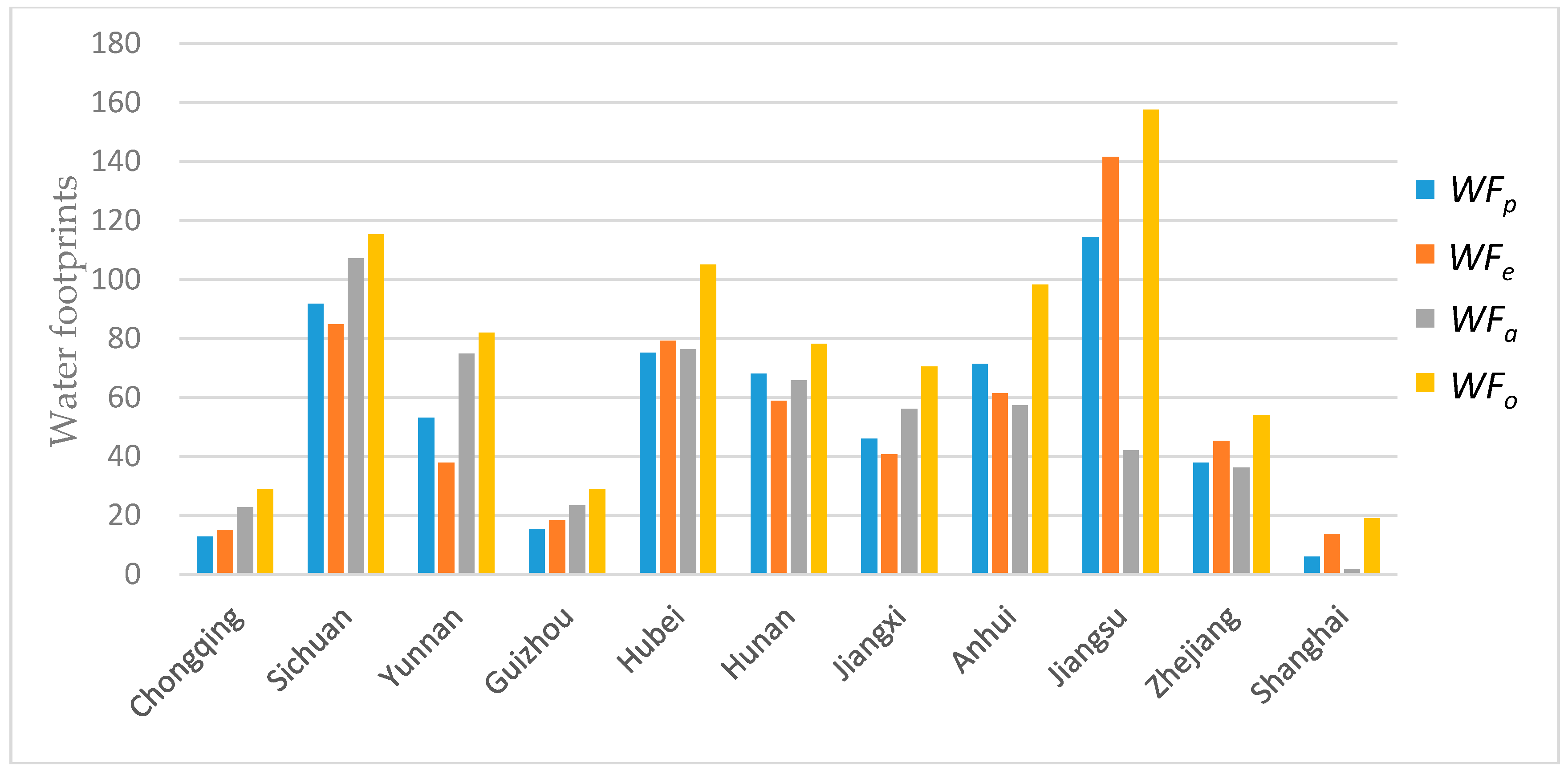
| WFo | WFp | WFe | WFa | |
|---|---|---|---|---|
| Chongqing | 28.83 | 12.81 | 15.04 | 22.78 |
| Sichuan | 115.29 | 91.83 | 84.77 | 107.22 |
| Yunnan | 82.00 | 53.13 | 37.84 | 74.79 |
| Guizhou | 29.00 | 15.34 | 18.42 | 23.45 |
| Hubei | 105.10 | 75.19 | 79.31 | 76.41 |
| Hunan | 78.21 | 68.10 | 58.89 | 65.76 |
| Jiangxi | 70.41 | 46.03 | 40.69 | 56.20 |
| Anhui | 98.25 | 71.37 | 61.46 | 57.42 |
| Jiangsu | 157.59 | 114.36 | 141.47 | 42.17 |
| Zhejiang | 54.02 | 37.81 | 45.32 | 36.16 |
| Shanghai | 19.04 | 6.03 | 13.71 | 1.74 |
| Sum of YREB | 837.951 | 592.01 | 596.92 | 564.09 |
| Upstream mean | 63.78 | 43.28 | 39.02 | 57.06 |
| Midstream mean | 84.57 | 63.11 | 59.63 | 66.12 |
| Downstream mean | 82.23 | 57.39 | 65.49 | 34.37 |
| Decreasing mean of YREB | - | 29.33% | 28.75% | 32.67% |
| T index | L index | G index | |
|---|---|---|---|
| WFp |  |  |  |
| WFe |  |  |  |
| WFa |  |  |  |
| Province | WA (billion m3) | WFO (billion m3) | WFOM (billion m3) | WFEM (billion m3) | IWSDO | IWSDOM | IWSDEM |
|---|---|---|---|---|---|---|---|
| Chongqing | 47.43 | 28.83 | 22.29 | 28.10 | 0.39 | 0.53 | 0.41 |
| Sichuan | 247.03 | 115.29 | 103.07 | 112.39 | 0.53 | 0.58 | 0.55 |
| Yunnan | 170.67 | 82.00 | 67.66 | 79.30 | 0.52 | 0.60 | 0.54 |
| Guizhou | 75.94 | 29.00 | 17.96 | 19.08 | 0.62 | 0.76 | 0.75 |
| Hubei | 79.01 | 105.10 | 58.91 | 81.41 | −0.33 | 0.25 | −0.03 |
| Hunan | 158.20 | 78.21 | 55.86 | 63.69 | 0.51 | 0.65 | 0.60 |
| Jiangxi | 142.40 | 70.41 | 42.16 | 50.84 | 0.51 | 0.70 | 0.64 |
| Anhui | 58.56 | 98.25 | 61.25 | 61.06 | −0.68 | −0.05 | −0.04 |
| Jiangsu | 28.35 | 157.59 | 134.68 | 97.70 | −4.56 | −3.75 | −2.45 |
| Zhejiang | 93.13 | 54.02 | 41.75 | 42.01 | 0.42 | 0.55 | 0.55 |
| Shanghai | 2.80 | 19.04 | 11.52 | 6.94 | −5.80 | −3.11 | −1.48 |
| Sum | 1103.52 | 837.75 | 617.11 | 642.52 | 0.24 | 0.44 | 0.42 |
| Decreasing mean of YREB | - | - | 26.2% | 23.3% | - | - | - |
© 2019 by the authors. Licensee MDPI, Basel, Switzerland. This article is an open access article distributed under the terms and conditions of the Creative Commons Attribution (CC BY) license (http://creativecommons.org/licenses/by/4.0/).
Share and Cite
Liu, G.; Hu, F.; Wang, Y.; Wang, H. Assessment of Lexicographic Minimax Allocations of Blue and Green Water Footprints in the Yangtze River Economic Belt Based on Land, Population, and Economy. Int. J. Environ. Res. Public Health 2019, 16, 643. https://doi.org/10.3390/ijerph16040643
Liu G, Hu F, Wang Y, Wang H. Assessment of Lexicographic Minimax Allocations of Blue and Green Water Footprints in the Yangtze River Economic Belt Based on Land, Population, and Economy. International Journal of Environmental Research and Public Health. 2019; 16(4):643. https://doi.org/10.3390/ijerph16040643
Chicago/Turabian StyleLiu, Gang, Fan Hu, Yixin Wang, and Huimin Wang. 2019. "Assessment of Lexicographic Minimax Allocations of Blue and Green Water Footprints in the Yangtze River Economic Belt Based on Land, Population, and Economy" International Journal of Environmental Research and Public Health 16, no. 4: 643. https://doi.org/10.3390/ijerph16040643