A Predictive Model for Steady State Ozone Concentration at an Urban-Coastal Site

 and
and 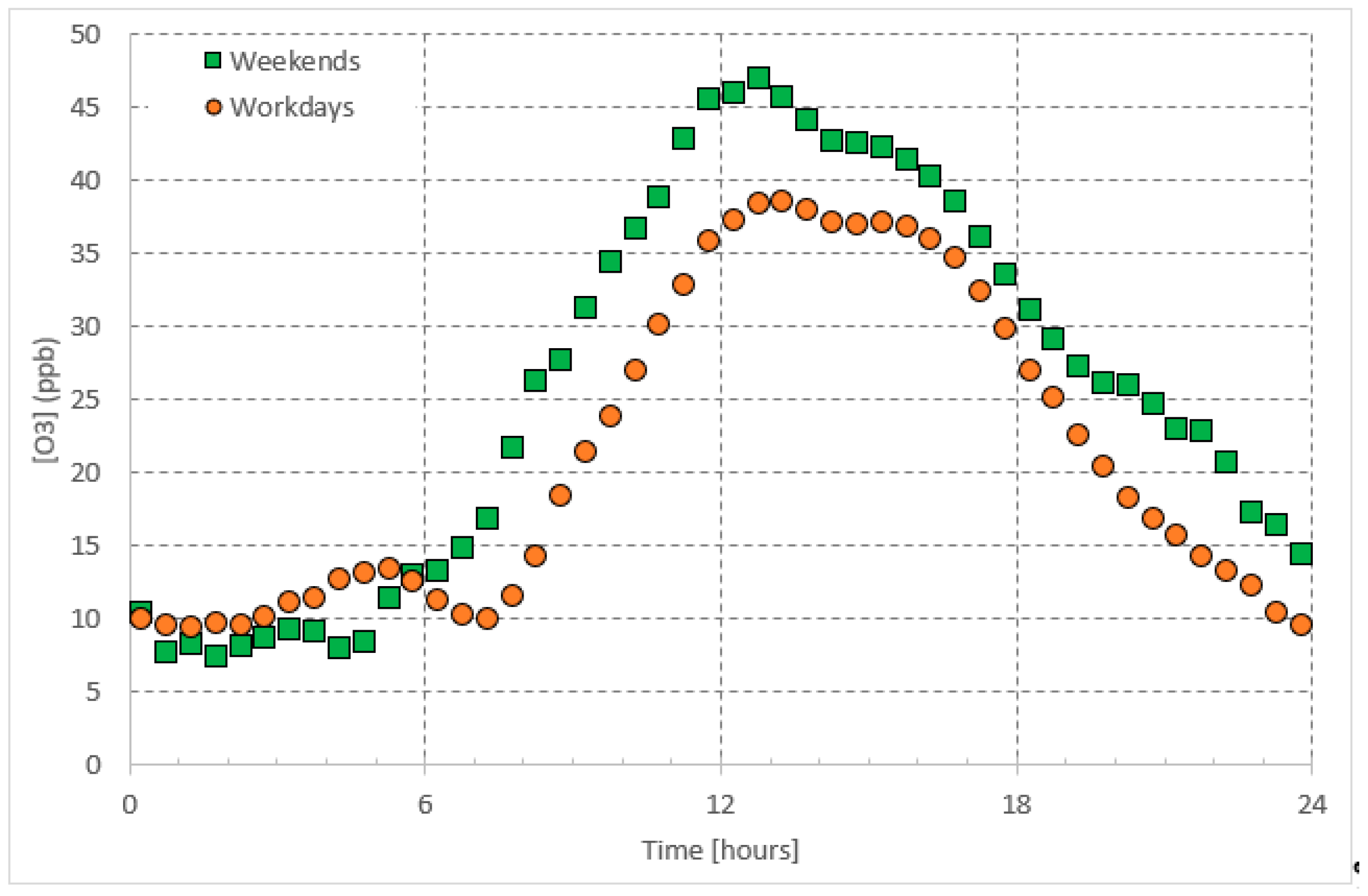
Abstract
:1. Introduction
2. Materials and Methods
2.1. Simple Statistical Predictive Model
2.2. Daytime Steady-State O3 Concentrations Prediction
2.3. Nighttime Steady-State O3 Concentrations Prediction
2.4. Data-Base
3. Results
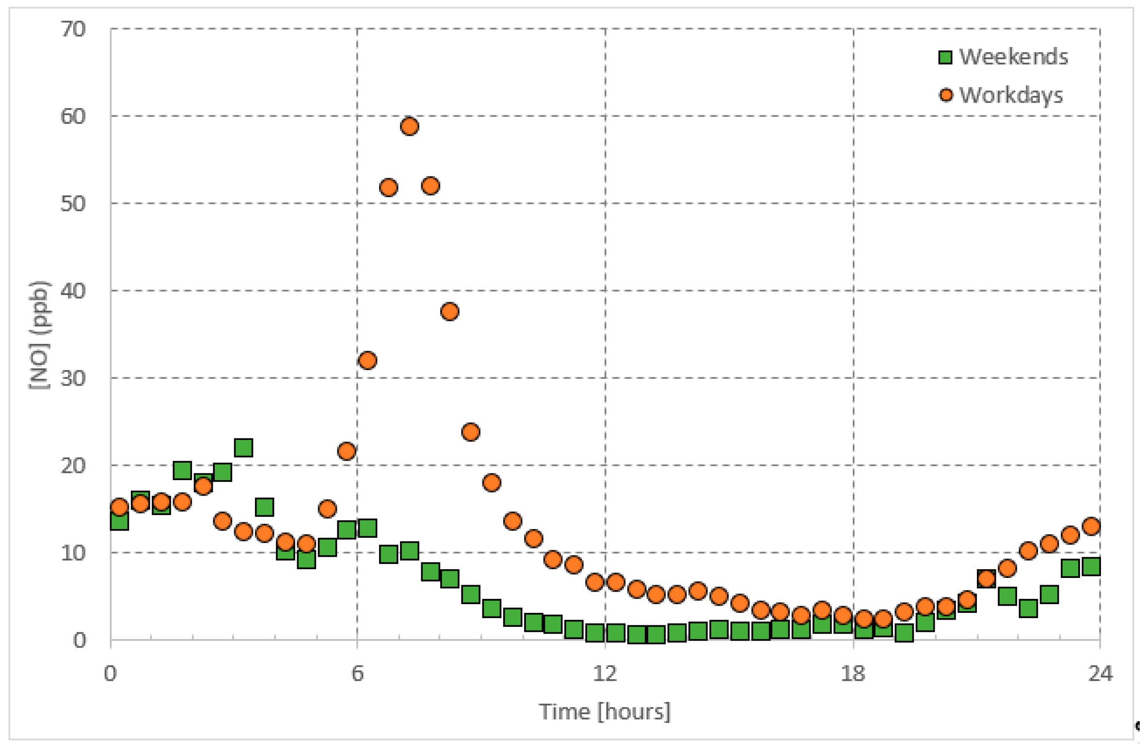
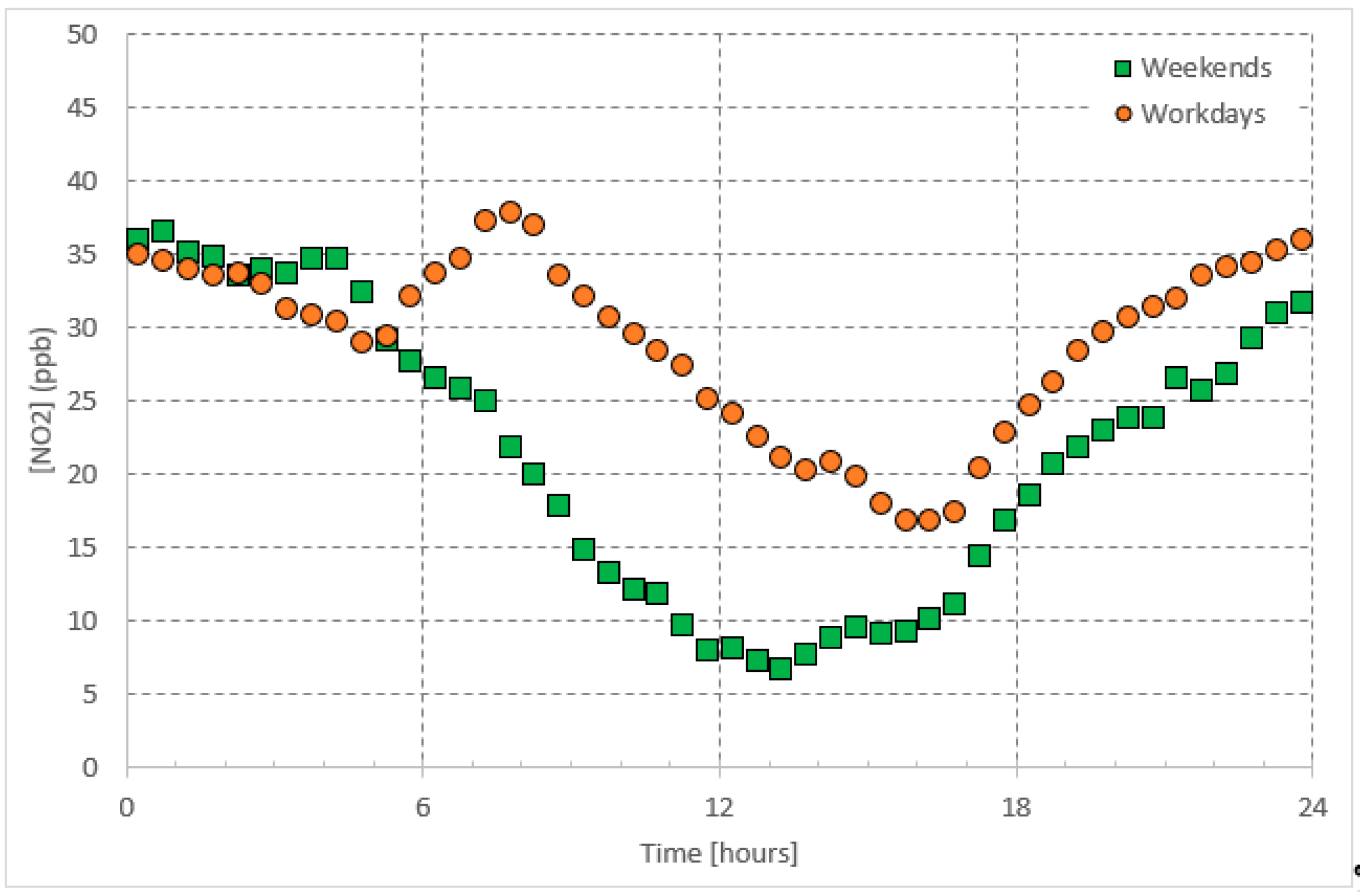
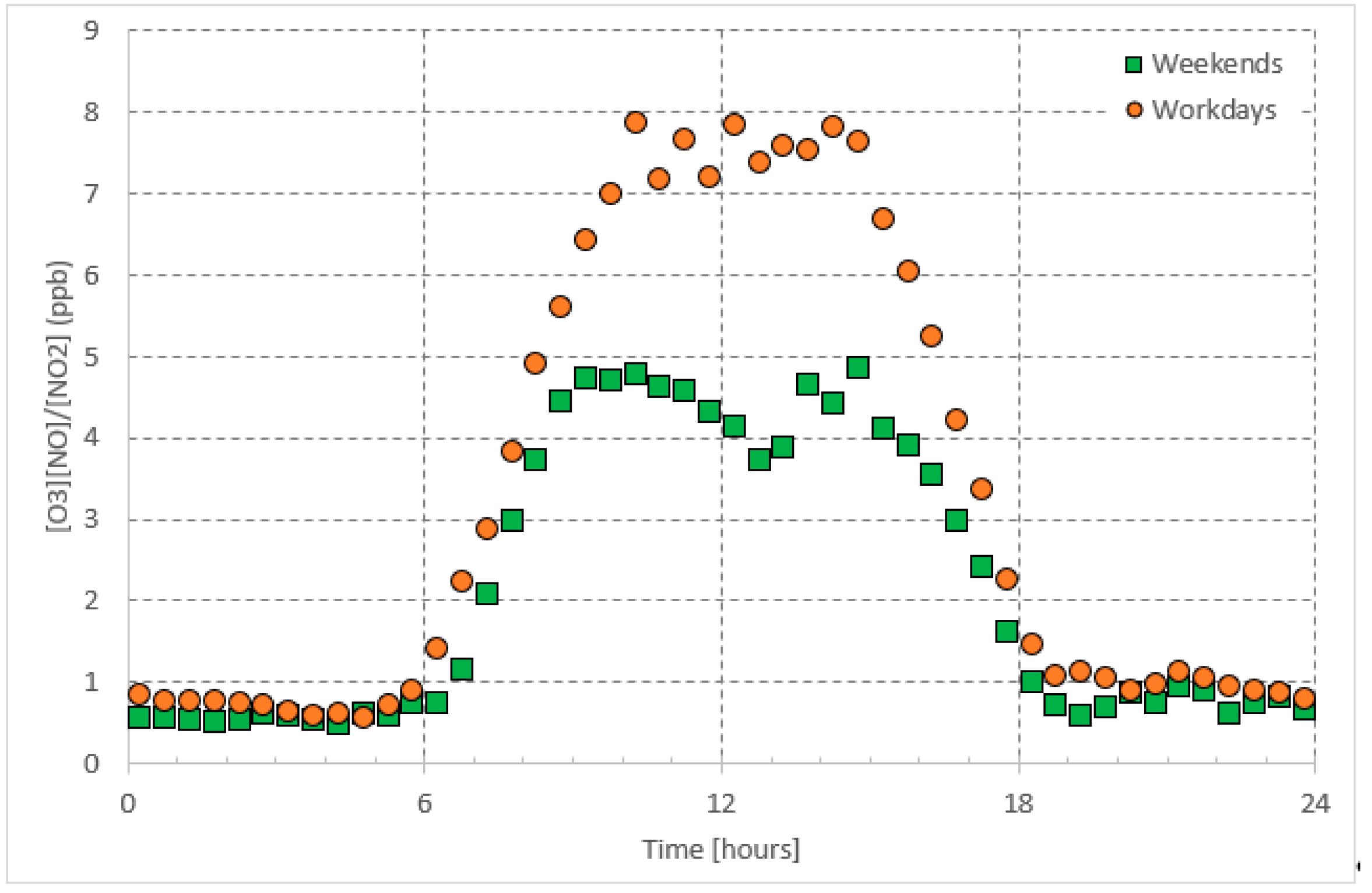
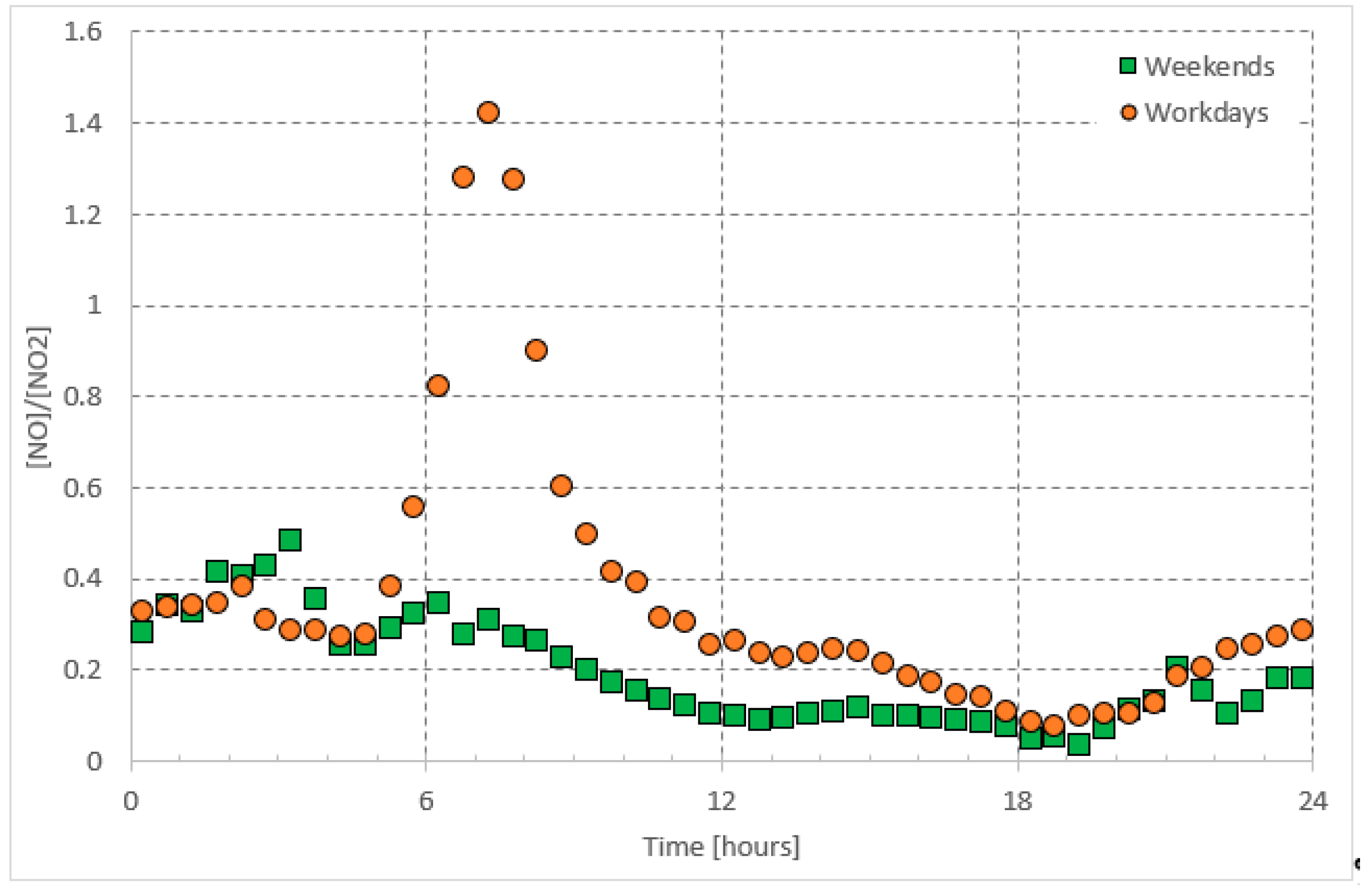
3.1. Overview of the Daily Patterns
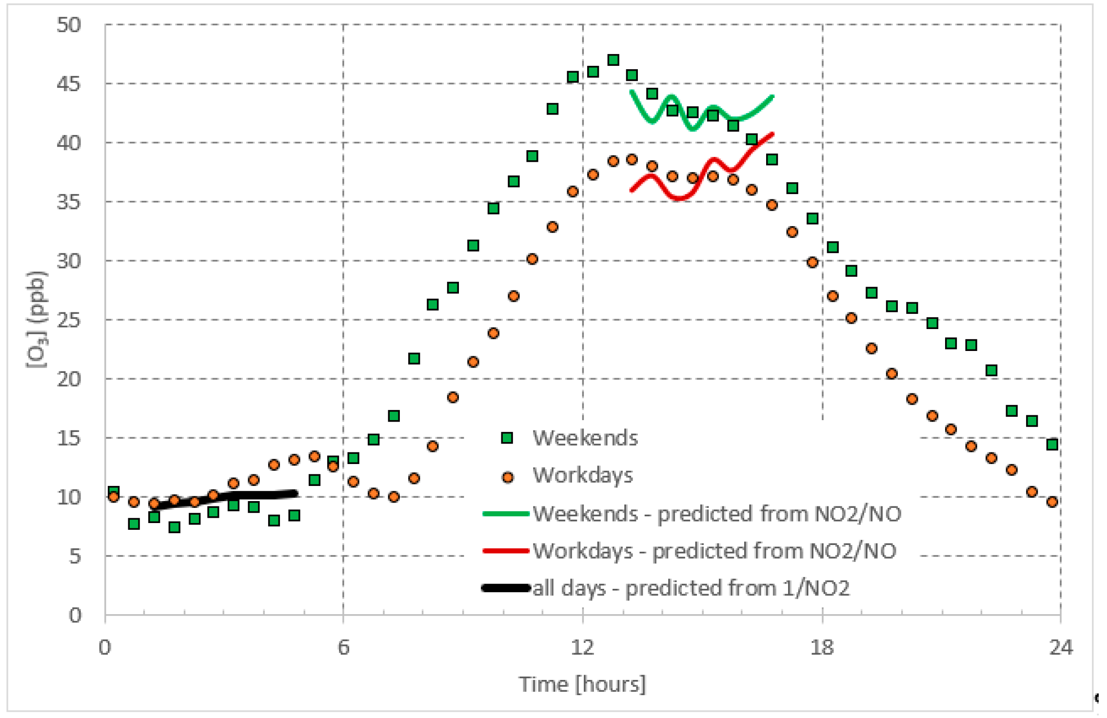
3.2. Prediction of Steady-State O3 Concentration
4. Conclusions
Author Contributions
Funding
Conflicts of Interest
References
- WHO. Health and Health Behaviour among Young People: Health Behaviour in School-Aged Children: A WHO Cross-National Study (HBSC), International Report; WHO: Geneva, Switzerland, 2000. [Google Scholar]
- IPCC. 2007: Summary for policymakers. In Climate Change 2007: Impacts, Adaptation and Vulnerability. Contribution of Working Group II to the Fourth Assessment Report of the Intergovernmental Panel on Climate Change; Cambridge University Press: Cambridge, UK, 2007; pp. 93–129. [Google Scholar]
- Thompson, A.M. The oxidizing capacity of the Earth’s atmosphere: Probable past and future changes. Science 1992, 256, 1157–1165. [Google Scholar] [CrossRef] [PubMed]
- Laurila, T. Observational study of transport and photochemical formation of ozone over northern Europe. J. Geophys. Res. Atmos. 1999, 104, 26235–26243. [Google Scholar] [CrossRef] [Green Version]
- Solomon, P.; Cowling, E.; Hidy, G.; Furiness, C. Comparison of scientific findings from major ozone field studies in North America and Europe. Atmos. Environ. 2000, 34, 1885–1920. [Google Scholar] [CrossRef]
- Thompson, A.M.; Witte, J.C.; Hudson, R.D.; Guo, H.; Herman, J.R.; Fujiwara, M. Tropical tropospheric ozone and biomass burning. Science 2001, 291, 2128–2132. [Google Scholar] [CrossRef] [PubMed]
- Pereira, M.; Alvim-Ferraz, M.; Santos, R. Relevant aspects of air quality in Oporto (Portugal): PM10 and O3. Environ. Monit. Assess. 2005, 101, 203–221. [Google Scholar] [PubMed]
- Tecer, L.; Ertürk, F.; Cerit, O. Development of a regression model to forecast ozone concentration in Istanbul City, Turkey. Fresenius Environ. Bull. 2003, 12, 1133–1143. [Google Scholar]
- Olszyna, K.; Luria, M.; Meagher, J. The correlation of temperature and rural ozone levels in southeastern USA. Atmos. Environ. 1997, 31, 3011–3022. [Google Scholar] [CrossRef]
- Vingarzan, R.; Taylor, B. Trend analysis of ground level ozone in the greater Vancouver/Fraser Valley area of British Columbia. Atmos. Environ. 2003, 37, 2159–2171. [Google Scholar] [CrossRef]
- Vukovich, F.M.; Sherwell, J. An examination of the relationship between certain meteorological parameters and surface ozone variations in the Baltimore–Washington corridor. Atmos. Environ. 2003, 37, 971–981. [Google Scholar] [CrossRef]
- Ribas, À.; Peñuelas, J. Temporal patterns of surface ozone levels in different habitats of the North Western Mediterranean basin. Atmos. Environ. 2004, 38, 985–992. [Google Scholar] [CrossRef]
- García, M.; Sánchez, M.; Pérez, I.; De Torre, B. Ground level ozone concentrations at a rural location in northern Spain. Sci. Total Environ. 2005, 348, 135–150. [Google Scholar] [CrossRef]
- Dueñas, C.; Fernández, M.; Cañete, S.; Carretero, J.; Liger, E. Assessment of ozone variations and meteorological effects in an urban area in the Mediterranean Coast. Sci. Total Environ. 2002, 299, 97–113. [Google Scholar] [CrossRef]
- Alvim-Ferraz, M.; Sousa, S.; Pereira, M.; Martins, F. Contribution of anthropogenic pollutants to the increase of tropospheric ozone levels in the Oporto Metropolitan Area, Portugal since the 19th century. Environ. Pollut. 2006, 140, 516–524. [Google Scholar] [CrossRef] [PubMed]
- Pudasainee, D.; Sapkota, B.; Shrestha, M.L.; Kaga, A.; Kondo, A.; Inoue, Y. Ground level ozone concentrations and its association with NOx and meteorological parameters in Kathmandu valley, Nepal. Atmos. Environ. 2006, 40, 8081–8087. [Google Scholar] [CrossRef]
- Sillman, S. The use of NOy, H2O2, and HNO3 as indicators for ozone-NOx-hydrocarbon sensitivity in urban locations. J. Geophys. Res. 1995, 100, 14175–114188. [Google Scholar] [CrossRef]
- Nevers, N. Control of volatile organic compounds (VOCs). Air Pollut. Control Eng. 2000, 18, 329–330. [Google Scholar]
- Sillman, S. The relation between ozone, NO x and hydrocarbons in urban and polluted rural environments. Atmos. Environ. 1999, 33, 1821–1845. [Google Scholar] [CrossRef]
- Guicherit, R.; Roemer, M. Tropospheric ozone trends. Chemosphere-Glob. Chang. Sci. 2000, 2, 167–183. [Google Scholar] [CrossRef]
- Tang, W.; Zhao, C.; Geng, F.; Peng, L.; Zhou, G.; Gao, W.; Xu, J.; Tie, X. Study of ozone “weekend effect” in Shanghai. Sci. China Ser. D Earth Sci. 2008, 51, 1354–1360. [Google Scholar] [CrossRef]
- Song, F.; Shin, J.Y.; Jusino-Atresino, R.; Gao, Y. Relationships among the springtime ground-level NOX, O3 and NO3 in the vicinity of highways in the US East Coast. Atmos. Pollut. Res. 2011, 2, 374–383. [Google Scholar] [CrossRef]
- Domínguez-López, D.; Adame, J.; Hernández-Ceballos, M.; Vaca, F.; De la Morena, B.; Bolívar, J. Spatial and temporal variation of surface ozone, NO and NO2 at urban, suburban, rural and industrial sites in the southwest of the Iberian Peninsula. Environ. Monit. Assess. 2014, 186, 5337–5351. [Google Scholar] [CrossRef] [PubMed]
- Finlayson-Pitts, B.J.; Pitts, J.N., Jr. Chemistry of the Upper and Lower Atmosphere: Theory, Experiments, and Applications; Academic Press: Cambridge, MA, USA, 1999. [Google Scholar]
- Rao, T.; Reddy, R.; Sreenivasulu, R.; Peeran, S.; Murthy, K.; Ahammed, Y.; Gopal, K.; Azeem, P.; Sreedhar, B.; Sunitha, K. Air space pollutants CO and NOx level at Anantapur (semi-arid zone), Andhra Pradesh. J. Indian Geophys. Union 2002, 3, 151–161. [Google Scholar]
- Rao, T.; Reddy, R.; Sreenivasulu, R.; Peeran, S.; Murthy, K.; Ahammed, Y.; Gopal, K.; Azeem, P.; Sreedhar, B.; Badarinath, K. Seasonal and diurnal variations in the levels of NOx and CO trace gases at Anantapur in Andhra Pradesh. J. Indian Geophys. Union 2002, 3, 163–168. [Google Scholar]
- Vingarzan, R. A review of surface ozone background levels and trends. Atmos. Environ. 2004, 38, 3431–3442. [Google Scholar] [CrossRef]
- Chameides, W.; Fehsenfeld, F.; Rodgers, M.; Cardelino, C.; Martinez, J.; Parrish, D.; Lonneman, W.; Lawson, D.; Rasmussen, R.; Zimmerman, P. Ozone precursor relationships in the ambient atmosphere. J. Geophys. Res. Atmos. 1992, 97, 6037–6055. [Google Scholar] [CrossRef]
- Lal, S.; Naja, M.; Subbaraya, B. Seasonal variations in surface ozone and its precursors over an urban site in India. Atmos. Environ. 2000, 34, 2713–2724. [Google Scholar] [CrossRef]
- Mazzeo, N.A.; Venegas, L.E.; Choren, H. Analysis of NO, NO2, O3 and NOx concentrations measured at a green area of Buenos Aires City during wintertime. Atmos. Environ. 2005, 39, 3055–3068. [Google Scholar] [CrossRef]
- Han, S.; Bian, H.; Feng, Y.; Liu, A.; Li, X.; Zeng, F.; Zhang, X. Analysis of the Relationship between O3, NO and NO2 in Tianjin, China. Aerosol Air Qual. Res. 2011, 11, 128–139. [Google Scholar] [CrossRef]
- Abdul-Wahab, S.A.; Bakheit, C.S.; Al-Alawi, S.M. Principal component and multiple regression analysis in modelling of ground-level ozone and factors affecting its concentrations. Environ. Model. Softw. 2005, 20, 1263–1271. [Google Scholar] [CrossRef]
- Sousa, S.; Martins, F.; Alvim-Ferraz, M.; Pereira, M.C. Multiple linear regression and artificial neural networks based on principal components to predict ozone concentrations. Environ. Model. Softw. 2007, 22, 97–103. [Google Scholar] [CrossRef]
- Özbay, B.; Keskin, G.A.; Doğruparmak, Ş.Ç.; Ayberk, S. Multivariate methods for ground-level ozone modeling. Atmos. Res. 2011, 102, 57–65. [Google Scholar] [CrossRef]
- Varotsos, C.; Ondov, J.; Efstathiou, M. Scaling properties of air pollution in Athens, Greece and Baltimore, Maryland. Atmos Environ. 2005, 39, 4041–4047. [Google Scholar]
- Alghamdi, M.; Khoder, M.; Harrison, R.M.; Hyvärinen, A.-P.; Hussein, T.; Al-Jeelani, H.; Abdelmaksoud, A.; Goknil, M.; Shabbaj, I.; Almehmadi, F. Temporal variations of O3 and NOx in the urban background atmosphere of the coastal city Jeddah, Saudi Arabia. Atmos. Environ. 2014, 94, 205–214. [Google Scholar] [CrossRef]
- Leighton, P. Photochemistry of Air Pollution; Elsevier: New York, NY, USA, 2012. [Google Scholar]
- Seinfeld, J.H.; Pandis, S.N. Atmospheric Chemistry and Physics: From Air Pollution to Climate Change; John Wiley & Sons: Hoboken, NJ, USA, 2016. [Google Scholar]
- Khodeir, M.; Shamy, M.; Alghamdi, M.; Zhong, M.; Sun, H.; Costa, M.; Chen, L.-C.; Maciejczyk, P. Source apportionment and elemental composition of PM2. 5 and PM10 in Jeddah City, Saudi Arabia. Atmos. Pollut. Res. 2012, 3, 331. [Google Scholar] [CrossRef] [PubMed]
- Marr, L.C.; Harley, R.A. Modeling the effect of weekday-weekend differences in motor vehicle emissions on photochemical air pollution in central California. Environ. Sci. Technol. 2002, 36, 4099–4106. [Google Scholar] [CrossRef]
- Kuang, S.; Newchurch, M.; Burris, J.; Wang, L.; Knupp, K.; Huang, G. Stratosphere-to-troposphere transport revealed by ground-based lidar and ozonesonde at a midlatitude site. J. Geophys. Res. Atmos. 2012, 117. [Google Scholar] [CrossRef] [Green Version]
- Cox, R.; Coker, G. Kinetics of the reaction of nitrogen dioxide with ozone. J. Atmos. Chem. 1983, 1, 53–63. [Google Scholar] [CrossRef]
- Huie, R.E.; Herron, J.T. The rate constant for the reaction O3 + NO2→O2 + NO3 over the temperature range 259–362 K. Chem. Phys. Lett. 1974, 27, 411–414. [Google Scholar] [CrossRef]
- Johnston, H.S.; Graham, R. Photochemistry of NOx and HNOx compounds. Can. J. Chem. 1974, 52, 1415–1423. [Google Scholar] [CrossRef]


© 2019 by the authors. Licensee MDPI, Basel, Switzerland. This article is an open access article distributed under the terms and conditions of the Creative Commons Attribution (CC BY) license (http://creativecommons.org/licenses/by/4.0/).
Share and Cite
Alghamdi, M.A.; Al-Hunaiti, A.; Arar, S.; Khoder, M.; Abdelmaksoud, A.S.; Al-Jeelani, H.; Lihavainen, H.; Hyvärinen, A.; Shabbaj, I.I.; Almehmadi, F.M.; et al. A Predictive Model for Steady State Ozone Concentration at an Urban-Coastal Site. Int. J. Environ. Res. Public Health 2019, 16, 258. https://doi.org/10.3390/ijerph16020258
Alghamdi MA, Al-Hunaiti A, Arar S, Khoder M, Abdelmaksoud AS, Al-Jeelani H, Lihavainen H, Hyvärinen A, Shabbaj II, Almehmadi FM, et al. A Predictive Model for Steady State Ozone Concentration at an Urban-Coastal Site. International Journal of Environmental Research and Public Health. 2019; 16(2):258. https://doi.org/10.3390/ijerph16020258
Chicago/Turabian StyleAlghamdi, Mansour A., Afnan Al-Hunaiti, Sharif Arar, Mamdouh Khoder, Ahmad S. Abdelmaksoud, Hisham Al-Jeelani, Heikki Lihavainen, Antti Hyvärinen, Ibrahim I. Shabbaj, Fahd M. Almehmadi, and et al. 2019. "A Predictive Model for Steady State Ozone Concentration at an Urban-Coastal Site" International Journal of Environmental Research and Public Health 16, no. 2: 258. https://doi.org/10.3390/ijerph16020258