Rubbertown Next Generation Emissions Measurement Demonstration Project

 , ,
, ,
Abstract
:
1. Introduction
2. Methods
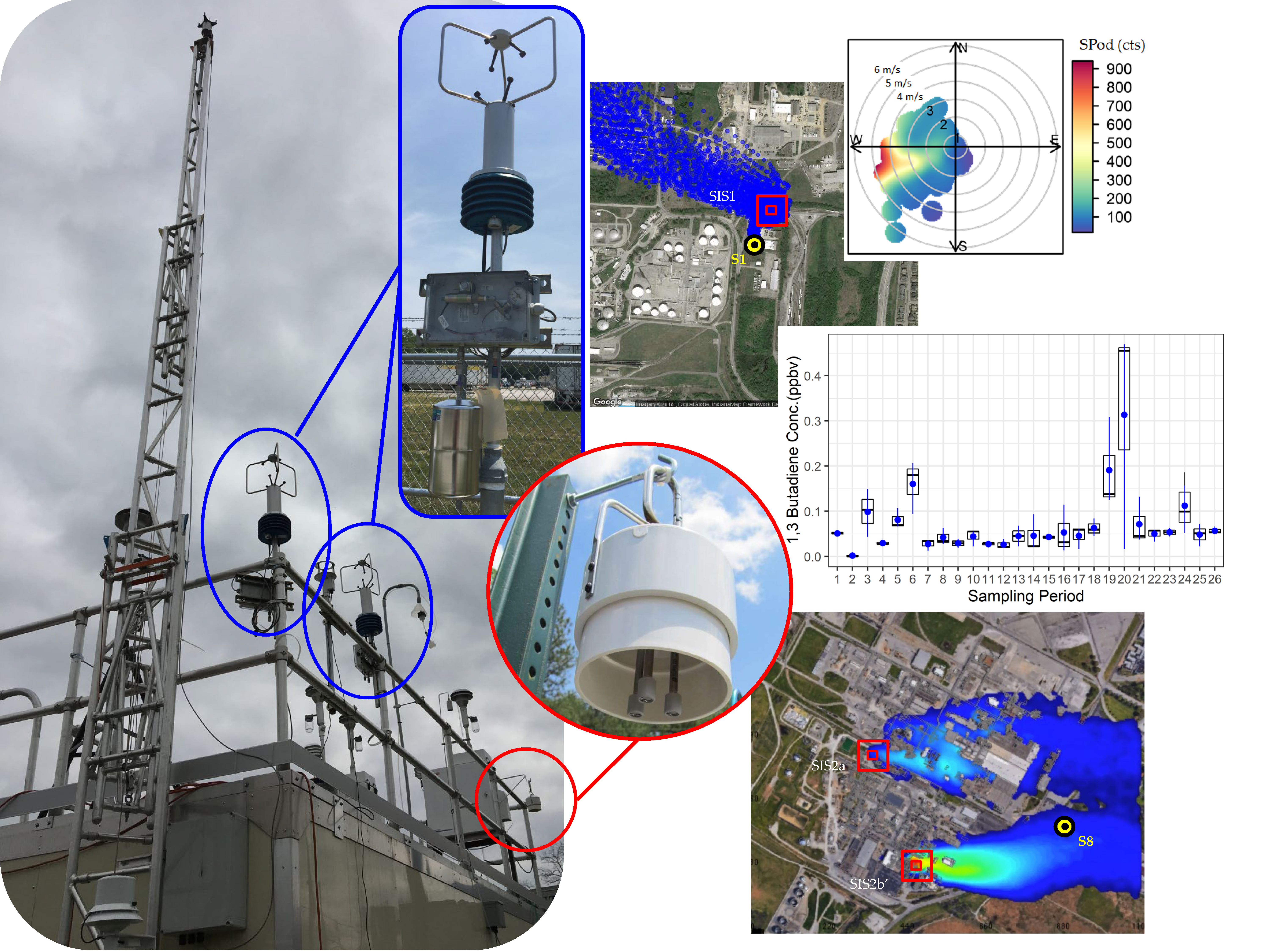
2.1. Sampling Locations
2.2. Passive Samplers (PSs)
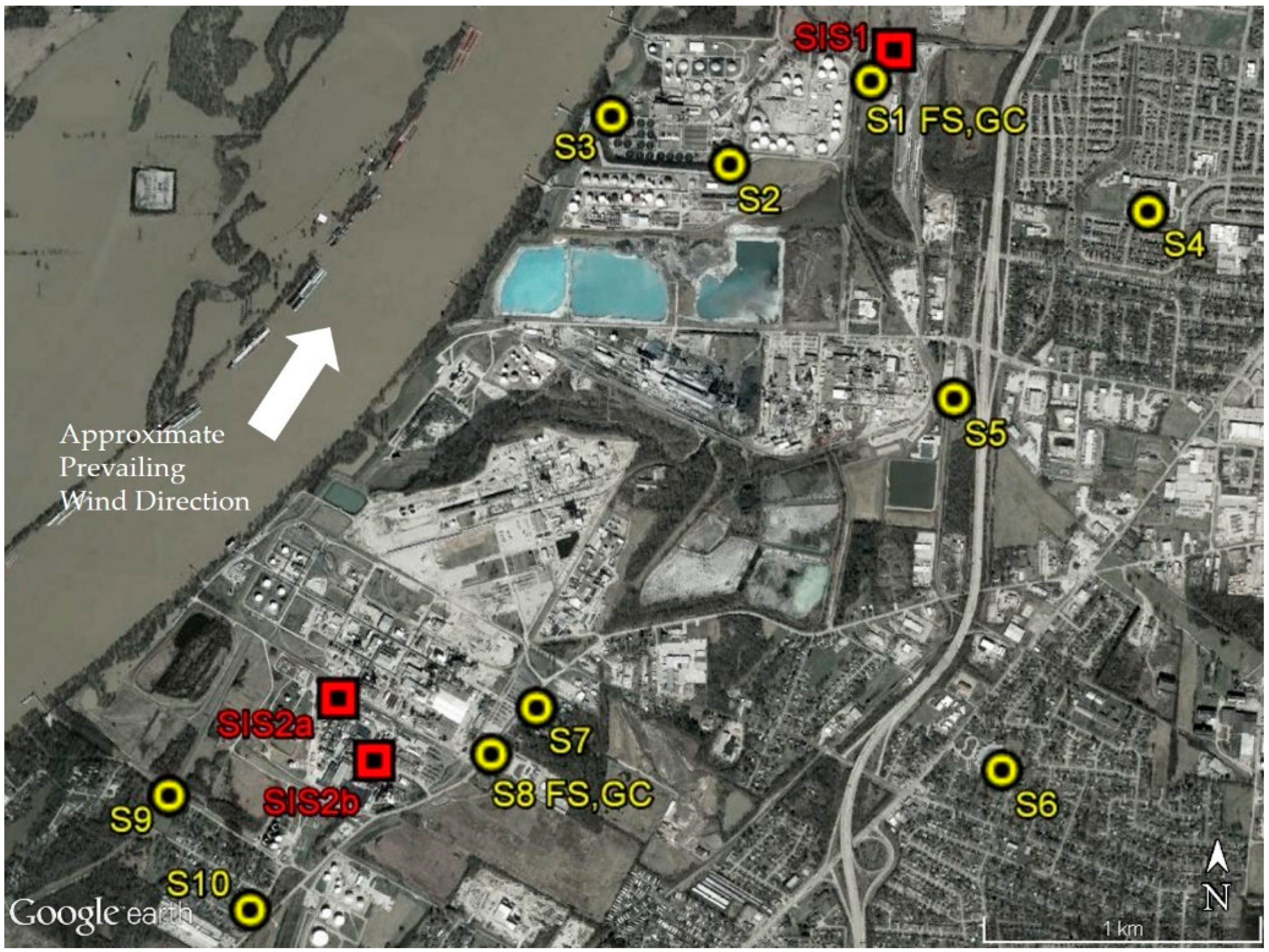
2.3. Fenceline Sensors (FSs)
2.4. Field Gas Chromatographs (GCs)
2.5. Source Location Models
3. Results and Discussion
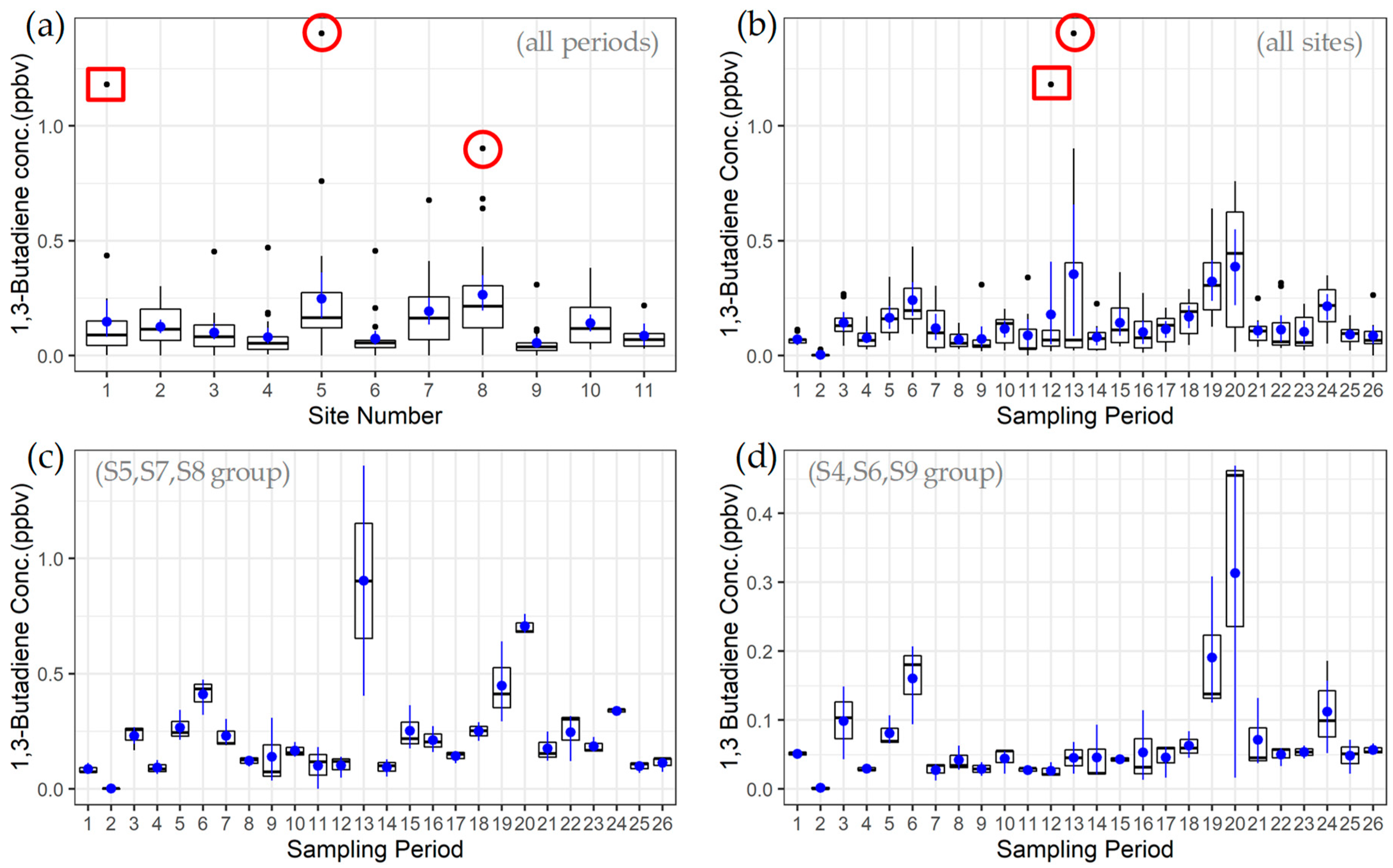
3.1. Passive Sampler Measurements
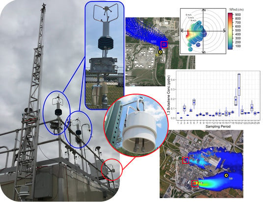
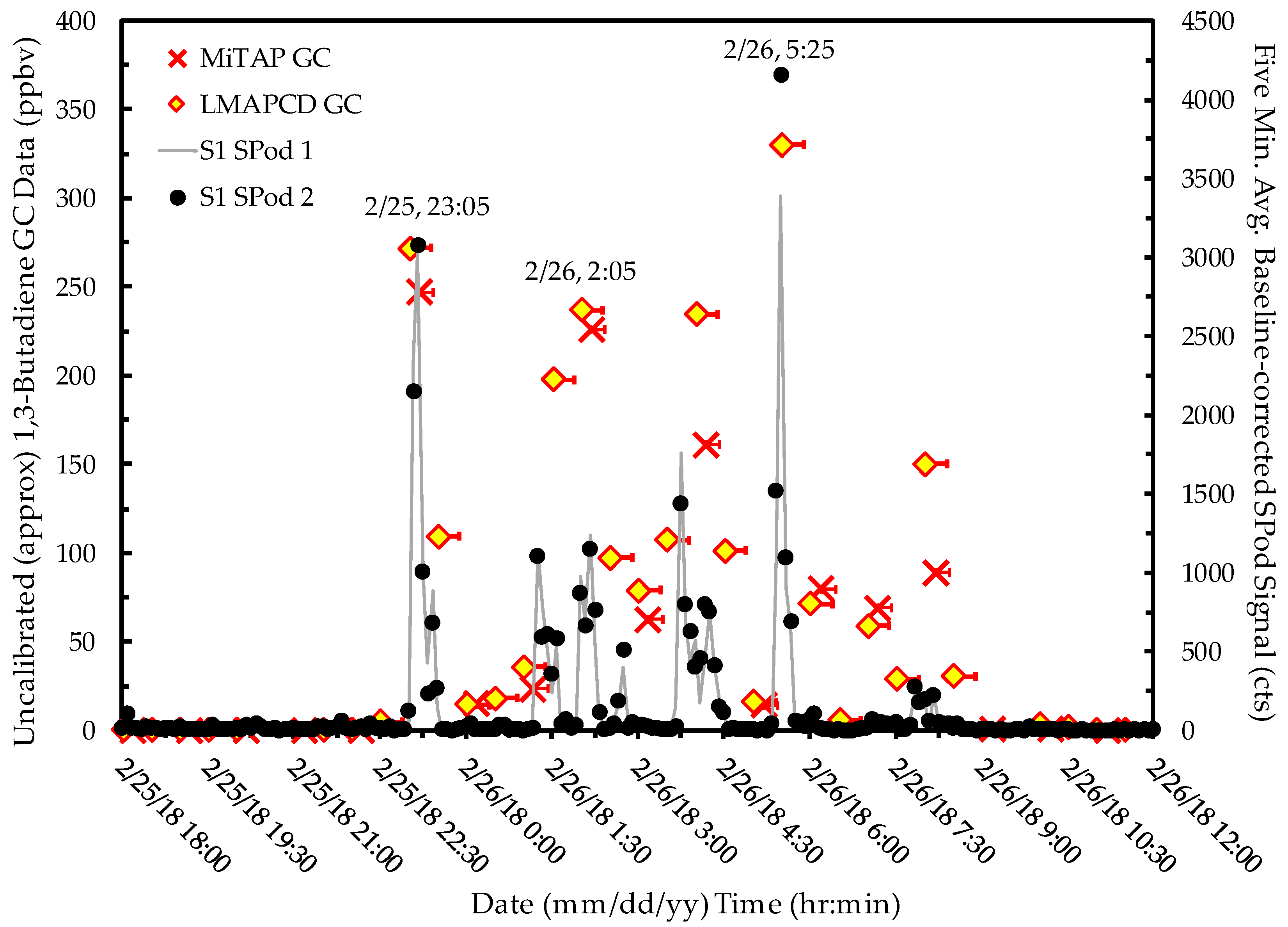
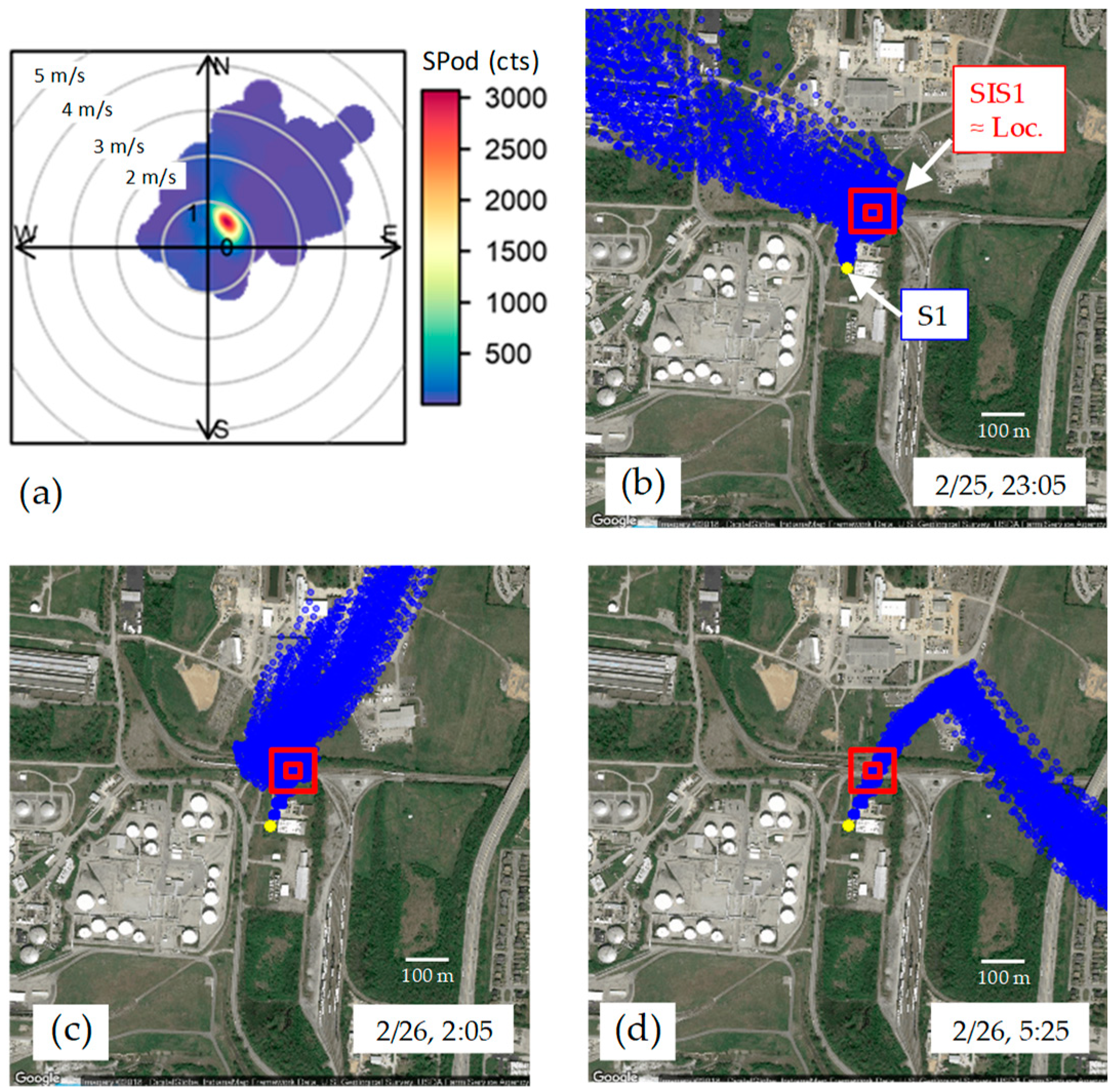
3.2. SIS1 Event
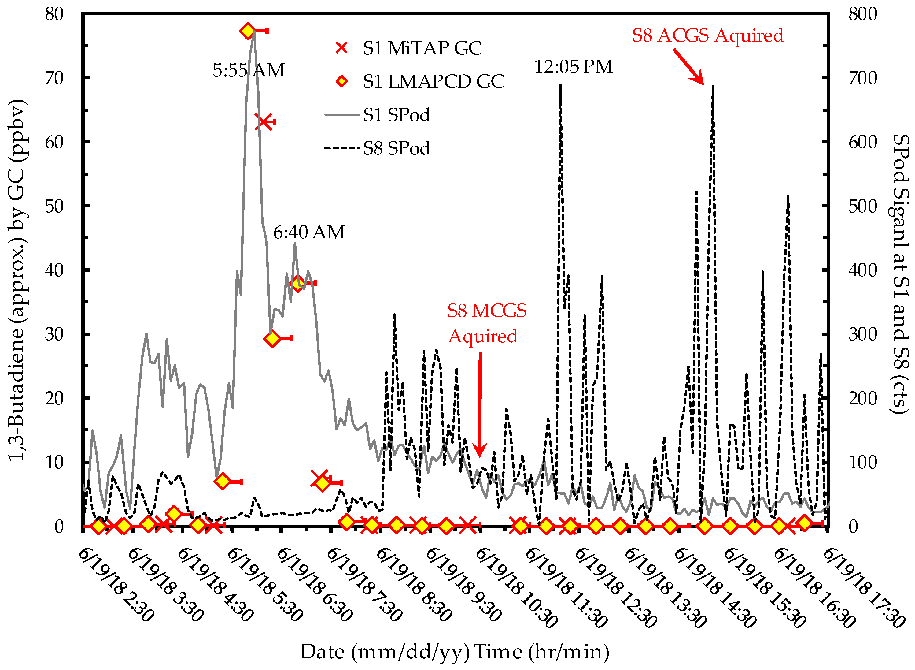
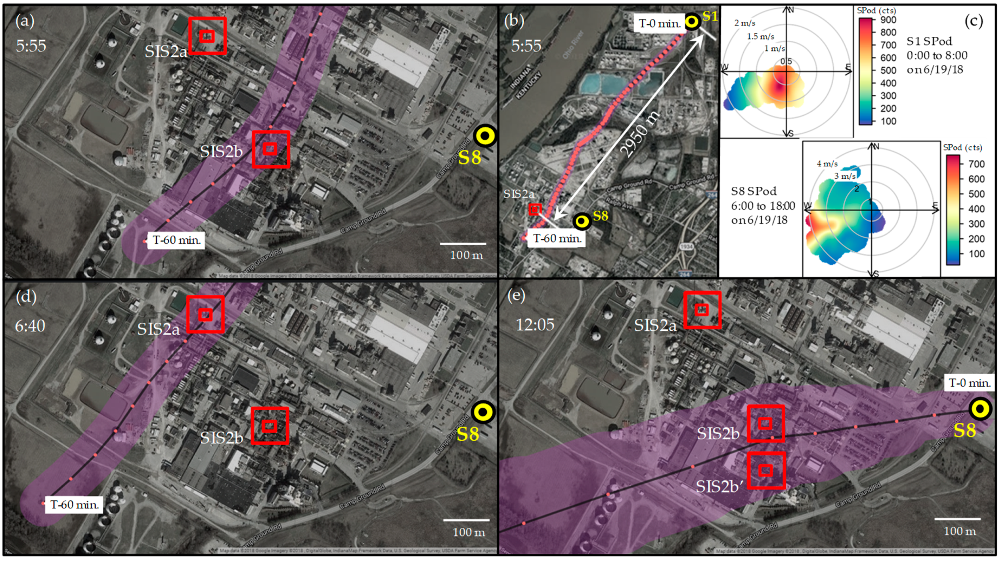
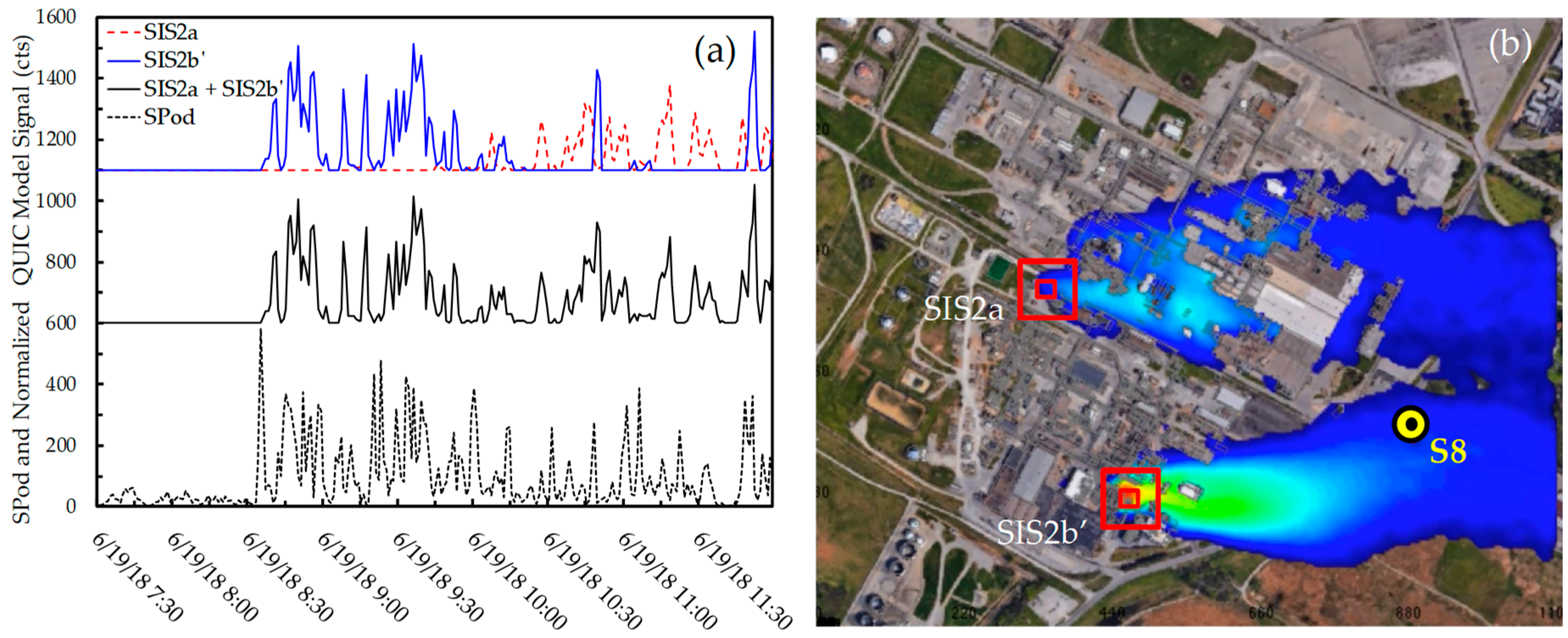
3.3. SIS2 Event
4. Conclusions
Supplementary Materials
Author Contributions
Funding
Acknowledgments
Conflicts of Interest
Acronyms and Abbreviations
| ACGS | automated canister grab sample |
| BAC | benchmark ambient concentration |
| BTM | back trajectory model |
| cts | counts |
| EPA | United States Environmental Protection Agency |
| FS | fenceline sensor |
| FTC | Firearms Training Center |
| GC | gas chromatograph |
| HAP | hazardous air pollutant |
| Hz | hertz (rate of once per second) |
| KY | Kentucky |
| km | kilometer |
| LMAPCD | City of Louisville Metro Air Pollution Control District |
| MCGS | manually activated canister grab sample |
| m | meters |
| m/s | meters per second |
| MDL | method detection limit |
| N | sample number |
| NATTS | National Air Toxics Trends Station |
| NGEM | next generation emissions measurement |
| ORD | Office of Research and Development |
| PID | photoionization detector |
| PN | part number |
| ppbv | part(s) per billion by volume |
| PS | passive sampler |
| QA | quality assurance |
| QUIC | Quick Urban & Industrial Complex |
| SD | secure digital |
| SDI | source direction indicator |
| s | standard deviation |
| SIS | stochastic industrial source |
| STAR | Strategic Toxic Air Reduction |
| SM | Supplementary Materials |
| TCTA | temporally combined trajectory analysis |
| TOF | time-of-flight |
| TO | toxic organics |
| μg/m3 | micrograms per cubic meter |
| USD | United States dollar |
| VOC | volatile organic compound |
| WLATS | West Louisville Air Toxics Study |
References
- Alvarez, R.A.; Zavala-Araiza, D.; Lyon, D.R.; Allen, D.T.; Barkley, Z.R.; Brandt, A.R.; Davis, K.J.; Herndon, S.C.; Jacob, D.J.; Karion, A. Assessment of methane emissions from the US oil and gas supply chain. Science 2018, 361, 186–188. [Google Scholar] [PubMed]
- McCoy, B.J.; Fischbeck, P.S.; Gerard, D. How big is big? How often is often? Characterizing Texas petroleum refining upset air emissions. Atmos. Environ. 2010, 44, 4230–4239. [Google Scholar] [CrossRef]
- Murphy, C.F.; Allen, D.T. Hydrocarbon emissions from industrial release events in the Houston-Galveston area and their impact on ozone formation. Atmos. Environ. 2005, 39, 3785–3798. [Google Scholar] [CrossRef]
- Xu, L.; Lin, X.; Amen, J.; Welding, K.; McDermitt, D. Impact of changes in barometric pressure on landfill methane emission. Glob. Biogeochem. Cycles 2014, 28, 679–695. [Google Scholar] [CrossRef] [Green Version]
- Small, C.C.; Cho, S.; Hashisho, Z.; Ulrich, A.C. Emissions from oil sands tailings ponds: Review of tailings pond parameters and emission estimates. J. Pet. Sci. Eng. 2015, 127, 490–501. [Google Scholar] [CrossRef]
- Piringer, M.; Knauder, W.; Petz, E.; Schauberger, G. Factors influencing separation distances against odour annoyance calculated by Gaussian and Lagrangian dispersion models. Atmos. Environ. 2016, 140, 69–83. [Google Scholar] [CrossRef]
- Fujita, E.M.; Campbell, D.E. Review of Current Air Monitoring Capabilities near Refineries in the San Francisco Bay Area; Report; Desert Research Institute for Bay Area Air Quality Management District; Desert Research Institute: Reno, NV, USA, 2013. [Google Scholar]
- Smith, R. Detect Them Before They Get Away: Fenceline Monitoring’s Potential To Improve Fugitive Emissions Management. Tulane Environ. Law J. 2015, 28, 433–453. [Google Scholar]
- Knighton, W.B.; Herndon, S.C.; Wood, E.C.; Fortner, E.C.; Onasch, T.B.; Wormhoudt, J.; Kolb, C.E.; Lee, B.H.; Zavala, M.; Molina, L. Detecting fugitive emissions of 1, 3-butadiene and styrene from a petrochemical facility: An application of a mobile laboratory and a modified proton transfer reaction mass spectrometer. Ind. Eng. Chem. Res. 2012, 51, 12706–12711. [Google Scholar] [CrossRef]
- Mellqvist, J.; Samuelsson, J.; Johansson, J.; Rivera, C.; Lefer, B.; Alvarez, S.; Jolly, J. Measurements of industrial emissions of alkenes in Texas using the solar occultation flux method. J. Geophys. Res. Atmos. 2010, 115, D00F17. [Google Scholar] [CrossRef]
- Olaguer, E.P.; Stutz, J.; Erickson, M.H.; Hurlock, S.C.; Cheung, R.; Tsai, C.; Colosimo, S.F.; Festa, J.; Wijesinghe, A.; Neish, B.S. Real time measurement of transient event emissions of air toxics by tomographic remote sensing in tandem with mobile monitoring. Atmos. Environ. 2017, 150, 220–228. [Google Scholar] [CrossRef]
- Stutz, J.; Pikelnaya, O. Demonstration of Remote Sensing Fenceline Monitoring Methods at Oil Refineries and Ports; South Coast Air Quality Management District: Diamond Bar, CA, USA, 2015.
- South Coast Air Qaulity Mangement District, Rule 1180; South Coast Air Quality Management District: Diamond Bar, CA, USA, 2017; Refinery Fenceline and Community Air Monitoring.
- U.S. EPA, Method 325A-Volatile Organic Compounds from Fugitive and Area Sources: Sampler Deployment and VOC Sample Collection. In 40 CFR Part 63, Subpart UUU[EPA-HQ-OAR-2010-0682; FRL-9720-4], RIN 2060-AQ75, Petroleum Refinery Sector Risk and Technology Review and New Source Performance Standards; U.S. Office of the Ferderal Regisiter: Washington, DC, USA, 2015; pp. 635–668.
- Snyder, E.G.; Watkins, T.H.; Solomon, P.A.; Thoma, E.D.; Williams, R.W.; Hagler, G.S.W.; Shelow, D.; Hindin, D.A.; Kilaru, V.J.; Preuss, P.W. The changing paradigm of air pollution monitoring. Environ. Sci. Technol. 2013, 47, 11369–11377. [Google Scholar] [CrossRef] [PubMed]
- Hanchette, C.; Lee, J.-H.; Aldrich, T.E. Asthma, Air Quality and Environmental Justice in Louisville, Kentucky. In Geospatial Analysis of Environmental Health; Springer: Dordrecht, The Netherlands, 2011; pp. 223–242. [Google Scholar]
- Barrett, M.; Combs, V.; Su, J.G.; Henderson, K.; Tuffli, M.; Collaborative, A.L. AIR Louisville: Addressing asthma with technology, crowdsourcing, cross-sector collaboration, and policy. Health Aff. 2018, 37, 525–534. [Google Scholar] [CrossRef] [PubMed]
- Sciences International Inc. West Louisville Air Toxics Study Risk Assessment, Final Report, Prepared for the Louisville Metro Air Pollution Control District; LMAPCD: Louisville, KY, USA, 2003. Available online: https://louisvilleky.gov/sites/default/files/air_pollution_control_district/documents/allother/apcd_-_west_louisville_air_toxins_-_2003.pdf (accessed on 6 June 2019).
- LMAPCD. Strategic Toxic Air Reduction (STAR) Program; LMAPCD: Louisville, KY, USA, 2005. Available online: https://louisvilleky.gov/government/air-pollution-control-district/strategic-toxic-air-reduction-program (accessed on 6 June 2019).
- LMAPCD. Ten Years Later: STAR & Louisville Air Toxics; LMAPCD: Louisville, KY, USA, 2015. Available online: https://louisvilleky.gov/sites/default/files/air_pollution_control_district/documents/allother/2015/star_board_presentation.pdf (accessed on 6 June 2019).
- LMAPCD. Rubbertown Sources; Google Maps; Interactive Map Viewer; Google: Mountain View, CA, USA, 2018; Available online: https://www.google.com/maps/d/viewer?mid=1w2Kwbam1jvoXpXTCiAFjUuyvqM0&ll=38.21627735761968%2C-85.83995283445205&z=14 (accessed on 6 June 2019).
- EPA, U.S. Method 325B-Volatile Organic Compounds from Fugitive and Area Sources: Sampler Preparation and Analysis; In 40 CFR Part 63, Subpart UUU [EPA-HQ-OAR-2010-0682; FRL-9720-4], RIN 2060-AQ75, Petroleum Refinery Sector Risk and Technology Review and New Source Performance Standards; U.S. Office of the Ferderal Regisiter: Washington, DC, USA, 2015; pp. 668–745.
- Mukerjee, S.; Smith, L.A.; Thoma, E.D.; Oliver, K.D.; Whitaker, D.A.; Wu, T.; Colon, M.; Alston, L.; Cousett, T.A.; Stallings, C. Spatial analysis of volatile organic compounds in South Philadelphia using passive samplers. J. Air Waste Manag. Assoc. 2016, 66, 492–498. [Google Scholar] [CrossRef] [PubMed] [Green Version]
- Oliver, K.D.; Cousett, T.A.; Whitaker, D.A.; Smith, L.A.; Mukerjee, S.; Stallings, C.; Thoma, E.D.; Alston, L.; Colon, M.; Wu, T. Sample integrity evaluation and EPA method 325B interlaboratory comparison for select volatile organic compounds collected diffusively on Carbopack X sorbent tubes. Atmos. Environ. 2017, 163, 99–106. [Google Scholar] [CrossRef] [PubMed]
- Thoma, E.D.; Brantley, H.L.; Oliver, K.D.; Whitaker, D.A.; Mukerjee, S.; Mitchell, B.; Wu, T.; Squier, B.; Escobar, E.; Cousett, T.A. South Philadelphia passive sampler and sensor study. J. Air Waste Manag. Assoc. 2016, 66, 959–970. [Google Scholar] [CrossRef] [PubMed] [Green Version]
- Thoma, E.D.; Miller, M.C.; Chung, K.C.; Parsons, N.L.; Shine, B.C. Facility fenceline monitoring using passive samplers. J. Air Waste Manag. Assoc. 2011, 61, 834–842. [Google Scholar] [CrossRef] [PubMed]
- Martin, N.A.; Duckworth, P.; Henderson, M.H.; Swann, N.R.; Granshaw, S.T.; Lipscombe, R.P.; Goody, B.A. Measurements of environmental 1,3-butadiene with pumped and diffusive samplers using the sorbent Carbopack X. Atmos. Environ. 2005, 39, 1069–1077. [Google Scholar] [CrossRef]
- U.S. EPA. Compendium Method TO-15, Compendium of Methods for the Determination of Toxic Organic Compounds in Ambient Air, 2nd ed.; Determination of Volatile Organic Compounds (VOCs) in Air Collected in Specially-Prepared Canisters and Analyzed by Gas Chromatography/Mass Spectrometry (GC/MS); EPA/625/R-96/010b; Center for Environmental Research Information, Office of Research and Development, U.S. EPA: Cincinnati, OH, USA, 1999.


| Project | Year | Site | N | Average (ppbv) | Median (ppbv) | σ (ppbv) | Max (ppbv) |
|---|---|---|---|---|---|---|---|
| NGEM | 2017/2018 | S1 | 26 | 0.15 | 0.09 | 0.23 | 1.18 |
| NGEM | 2017/2018 | S1 1 | 25 | 0.11 | 0.08 | 0.09 | 0.44 2 |
| WLATS | 2001 | A (S1) | 4 | 0.86 | 0.54 | 0.92 | 2.19 |
| WLATS | 2002 | A (S1) | 30 | 1.03 | 0.59 | 1.24 | 4.81 |
| WLATS | 2003 | A (S1) | 34 | 1.53 | 0.71 | 1.94 | 6.62 |
| WLATS | 2004 | A (S1) | 29 | 0.73 | 0.16 | 1.22 | 5.28 |
| WLATS | 2005 | A (S1) | 31 | 1.05 | 0.79 | 1.16 | 4.69 |
| NGEM | 2017/2018 | S6 | 26 | 0.07 | 0.05 | 0.09 | 0.462 |
| WLATS | 2001 | F(S6) | 6 | 0.40 | 0.42 | 0.23 | 0.72 |
| WLATS | 2002 | F(S6) | 31 | 0.81 | 0.33 | 1.30 | 7.01 |
| WLATS | 2003 | F(S6) | 38 | 0.72 | 0.23 | 1.10 | 5.09 |
| WLATS | 2004 | F(S6) | 29 | 0.42 | 0.16 | 0.54 | 2.18 |
| WLATS | 2005 | F(S6) | 31 | 1.00 | 0.31 | 1.57 | 7.34 |
© 2019 by the authors. Licensee MDPI, Basel, Switzerland. This article is an open access article distributed under the terms and conditions of the Creative Commons Attribution (CC BY) license (http://creativecommons.org/licenses/by/4.0/).
Share and Cite
Thoma, E.; George, I.; Duvall, R.; Wu, T.; Whitaker, D.; Oliver, K.; Mukerjee, S.; Brantley, H.; Spann, J.; Bell, T.; et al. Rubbertown Next Generation Emissions Measurement Demonstration Project. Int. J. Environ. Res. Public Health 2019, 16, 2041. https://doi.org/10.3390/ijerph16112041
Thoma E, George I, Duvall R, Wu T, Whitaker D, Oliver K, Mukerjee S, Brantley H, Spann J, Bell T, et al. Rubbertown Next Generation Emissions Measurement Demonstration Project. International Journal of Environmental Research and Public Health. 2019; 16(11):2041. https://doi.org/10.3390/ijerph16112041
Chicago/Turabian StyleThoma, Eben, Ingrid George, Rachelle Duvall, Tai Wu, Donald Whitaker, Karen Oliver, Shaibal Mukerjee, Halley Brantley, Jane Spann, Tiereny Bell, and et al. 2019. "Rubbertown Next Generation Emissions Measurement Demonstration Project" International Journal of Environmental Research and Public Health 16, no. 11: 2041. https://doi.org/10.3390/ijerph16112041