2.2. Questionnaire and Definition of Cardiovascular Disease
A standardized questionnaire was applied to obtain personal data related to potential risk factors of CVD. These factors included age, gender, height, weight, cigarette smoking, alcohol drinking, tea and coffee consumption, daily salt intake, exercise habits, and family history of hypertension. All subjects’ lifestyle habits were defined in detail to avoid information bias. Current cigarette smokers were defined as subjects who admitted to smoking at least three times per week for more than six months. Similar definitions were used to classify current alcohol drinkers, and tea and coffee consumers. Participants were considered to have high salt intake if they reported that they consumed more dietary salt than other study subjects based on the median consumption. Regular exercisers were defined as those who participated in exercise at least three times per week for six months or more. A family history of hypertension was positive if the subject reported to have parents or grandparents with doctor-diagnosed hypertension. Additionally, body weight (kg) was divided with the square of the height (m2) to calculate body mass index (BMI) for each subject.
Participants were regarded as a case of CVD if he/she answered affirmatively to the question: “Have you been diagnosed with CVD by a physician in the past while living at the current address?” Among the 663 subjects in this study, 46 cases were identified using this criterion. Accordingly, the participants were classified into a case group of 46 subjects and a control group of the remaining 617 subjects.
2.3. Road Traffic Noise Measurements and Traffic Calculations
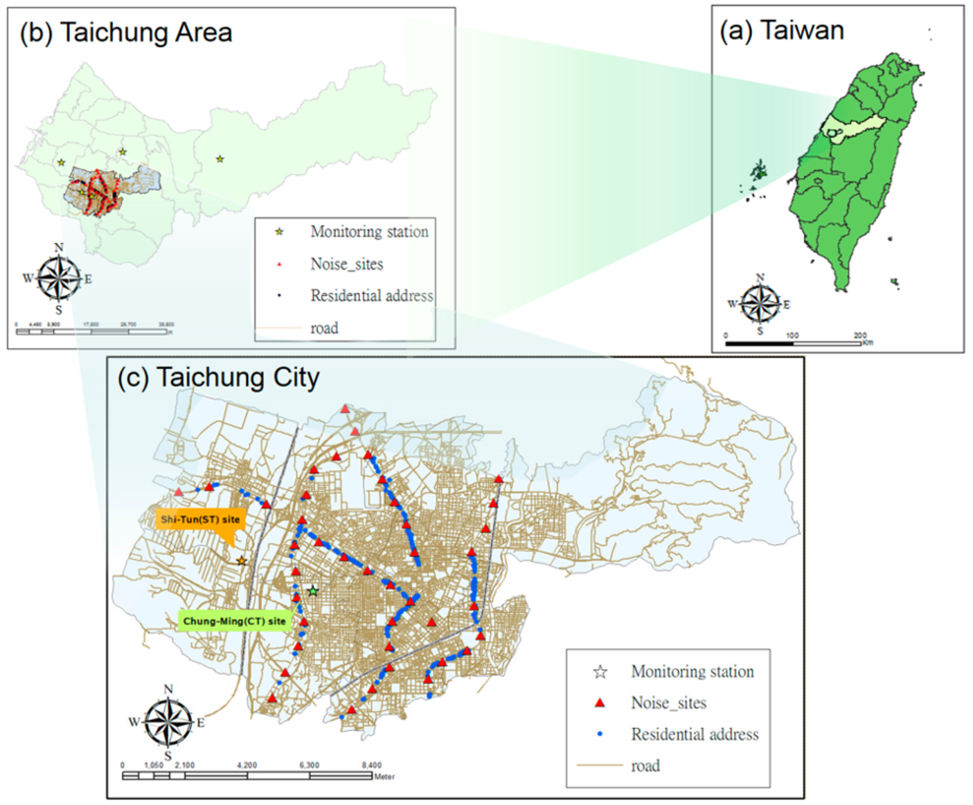
Road traffic noise levels were determined using an octave-band analyzer (TES-1358, TES Electronic Corp., Taipei, Taiwan), which can report 1-s to 24-h continuous equivalent sound levels (Leq) in the range of 30–130 A-weighted decibels (dBA) and time-weighted average (TWA) noise levels. Before conducting the noise measurements, a sound-level calibrator (TES-1356, TES Electronic Corp., Taipei, Taiwan) was used to calibrate this equipment. We set up 42 sampling sites at 1-km intervals along each of four main roads, and located these sampling sites 1 m away from buildings with a height of 1.5 m from the ground. Two industrial hygienists measured 15-min TWA Leq at each sampling site on weekdays from 9:00–17:00. All subjects were divided into 42 groups based on the closest sampling site to assign their daily exposure to road traffic noise levels. The distance between the sampling site and a subject’s address ranged from 5.2 m to 67.7 m within each group. Each participant was assigned to one value of road traffic noise exposure that corresponded with the 8-h TWA Leq (LAeq,8h) measured at the closest site.
During the monitoring period, two research assistants evaluated traffic flow rates of heavy-duty diesel trucks (≥3.5 ton), light-duty diesel trucks (<3.5 ton), light-duty gasoline vehicles (<3.5 ton), and motorcycles at each of 42 sampling sites. Each assistant was responsible for calculating two types of traffic vehicles passing in front of the sampling sites. The sum of motorcycles, light-duty gasoline vehicles, light-duty diesel trucks, and heavy-duty diesel trucks was used for total traffic flow rate in this study.
2.5. Statistical Analysis
We first used the Shapiro–Wilk test to determine the normality of the continuous variables, including age, BMI, LAeq,8h, PM10, and NO2 levels. Because statistical p values for these variables were less than 0.001 among all participants that showed non-normal distribution, the Wilcoxon signed rank sum test was performed to examine univariate comparisons between different groups for continuous variables. In addition, the Chi-square test was applied to compare the differences between groups for dichotomous variables. The Spearman rank correlation was used to investigate the correlations between road traffic noise, air pollutants, and total traffic among subjects.
Continuous (i.e., 5-dBA increase in road traffic noise, 1 µg/m
3 increase in PM
10, and 1 ppb increase in NO
2) and categorical variables (i.e., high-exposure group versus low-exposure group) of road traffic noise and air pollutants among participants were used to examine the association with the prevalence of CVD. We used 80 dBA as the cut-off value for noise exposure categories because exposure to L
Aeq,8h ≥ 80 dBA has been reported to be associated with an increased prevalence of hypertension among residents [
13]. The median value for PM
10 (58 µg/m
3) was used to divide subjects into high- and low-exposure groups with a similar number in each subgroup, because participants being exposed to PM
10 (ranged 57–59 μg/m
3) levels was higher than air quality annual guidelines of the World Health Organization (WHO) (PM
10: 20 μg/m
3) [
16], while still lower than the Taiwan annual standard of air quality (65 μg/m
3) [
17]. We selected 20 ppb as the cut-off value for NO
2 exposure categories based on the WHO guideline (NO
2: 40 μg/m
3, equal to 19.5 ppb at 1 atmosphere, 0 °C) [
16]. Accordingly, 663 participants were further separated into co-exposure to high-noise and high-air pollutants group, high-noise and low-air pollutants group, low-noise and high-air pollutants group, and low-noise and low-air pollutants group to investigate the interaction.
We used logistic regression models to calculate odds ratios (ORs) and 95% confidence intervals (CIs) in this study. For each combination of high and low exposure groups for road traffic noise, PM
10 and NO
2, the crude OR of self-reported CVD in participants above versus below the median exposure were calculated by simple logistic regression models. We used the following selection process to identify covariates in the best fit model. First, a full model was constructed with the outcome variable of CVD prevalence and all covariates. We applied the forward method with an entry level of 0.10 and identified three variables (i.e., age, BMI, and family history of hypertension) significantly associated with the outcome (all
p values < 0.05). These covariates were then included in a reduced model. Finally, every possible combination of remaining variables (i.e., gender, cigarette smoking, and alcohol, tea and coffee consumption, regular exercise, salt intake) was added to the reduced model, and the Akaike information criterion (AIC) of these models was compared. Based on this criterion, three variables of age, BMI, and family history of hypertension were kept with the lowest AIC to create the final adjusted model. In addition to these three variables, five important risk factors of CVD reported in the literature [
18,
19,
20], including gender, cigarette smoking, alcohol consumption, salt intake, and physical inactivity, were included in the multivariable logistic regression as the final model. Model selection was repeated for every combination of exposure variables (i.e., dichotomous high- vs. low-exposure groups or four different co-exposure groups) and the outcome to ensure similar selection of covariates.
We also present the ORs and 95% CI to show the risk of CVD prevalence per 5-dBA increase in noise, 1 μg/m
3 increase in PM
10, and 1 ppb increase in NO
2 exposure in the single-exposure models. In order to investigate the interaction between road traffic noise and air pollutants exposure, both noise and PM
10 (or NO
2) were included simultaneously in a multivariable logistic regression (two-exposure model) to compare the differences in exposure-effect estimates before and after mutual adjustment. The C statistic value was used to show the concordance between the model estimate and the observed case of CVD [
21] and the Hosmer and Lemeshow method was applied for the goodness-of-fit test. C statistic values higher than 0.7 were generally considered fair and clinically useful [
21] and the probability of the Hosmer and Lemeshow test greater than 0.05 indicated the goodness of fit for the model. The variance inflation factor (VIF) was used to test the multi-collinearity in the regression models and a VIF value of 3 was selected as the cut-off point to indicate multi-collinearity [
22]. Neither of the interaction term of noise and PM
10 nor of noise and NO
2 were not included in the two-exposure models because of the severe multi-collinearity (both VIF values > 10). Instead, the total traffic was put in the single-exposure and two-exposure models to control for other air pollutants. We used the SAS standard package for Windows version 9.2 (SAS Institute Incorporation, Cary, NC, USA) to perform statistical analyses and set the significance level at 0.05 for all statistical tests in the present study.


 and
and 
