1. Introduction
Multi-attribute decision-making is a problem in which a decision-maker evaluates a finite set of alternatives associated with multiple attributes. It is widely used in various areas such as management [
1,
2], the environment [
3], economy [
4,
5], technology [
6] and engineering [
7,
8]. Due to the uncertainty of the actual decision-making environment and the limitations of human cognition, the decision-making information usually consists of grey numbers for a decision maker in the evaluation of the alternatives, such as interval grey numbers [
9,
10] and extended grey numbers [
11]. With the aggravation of the environmental complexity, the decision-making problem also requires multi-source decision information to evaluate the potential alternatives objectively and comprehensively. However, the diversity of information sources often forms a heterogeneous data sequence that contains different types of data. In this case, the traditional single type of grey information can no longer meet the requirements of the actual modeling. Therefore, grey multi-source heterogeneous data are presented, which can deal with higher complexity and uncertainty to describe the potential alternative’s comprehensive performance more accurately.
Nowadays, the current research about the multi-attribute decision-making method has resulted in many significant achievements, such as AHP [
12], TODIM [
13], ELECTRE III [
14], TOPSIS [
15] and VIKOR [
16]. Grey relational analysis (GRA) is an effective method to solve multi-attribute decision-making problem in grey system theory [
17]. Its basic idea is to judge whether or not different data sequences are closely associated according to the geometric shapes of their sequence curves. The more similar the curves are, the greater the grey relational degree is, and vice versa. The GRA method has the advantages that it is unnecessary to take the sample size and typical distribution regularity into consideration. At present, this method has been widely used in practice. Kolhapure et al. [
18] used the GRA method to study the problem of geometrical optimization of strain gauge force transducers. Kirubakaran and Ilangkumaran [
19] developed a hybrid MADM model which combined FAHP, GRA and TOPSIS to select an optimum maintenance strategy. Li and Zhao [
20] integrated GRA and VIKOR for evaluating performance of industrial plants. Liu et al. [
21] proposed a dynamic fuzzy GRA method to select emergency treatment technology. In addition, many scholars also improved the GRA method theoretically, including the optimization of several GRA models [
22], the construction of grey relational degree [
23] and the weights determination in GRA [
24]. Throughout the relevant literature of GRA, whether it is related to application or to methodological research, the employed attribute values usually form a single type of decision-making information. But in the case of GRA whose attribute values are a mixture of different data types of grey information from multiple sources, the study is still relatively scarce. Therefore, we extend the GRA method to accommodate grey multi-source heterogeneous data.
Additionally, in practical decision-making, the decision problem usually presents a multi-attribute multi-level decision-making structure, and the evaluation attributes are not entirely independent, but mostly causal. Most of the existing decision-making methods assume that the attributes are independent of each other, and the causalities between attributes are neglected. Decision Making Trial and Evaluation Laboratory (DEMATEL) is a method for analyzing complex system factors. It can recognize the causalities between complex social factors and identify the key elements based on graph theory [
25]. In the DEMATEL method, the attributes are divided into a set of cause attributes and a set of effect attributes, wherein the cause attributes have a certain influence on the effect attributes. According to the influencing relationships, the relative importance between attributes can be determined. It can be seen that the DEMATEL method can effectively handle the causalities between attributes and determine the attribute weights. At present, the DEMATEL method has been widely applied in the fields of green supply chain management [
26], sustainable supply chain management [
27], sustainable consumption and production [
28], risk analysis [
29] and other fields. The determination of the initial direct relation matrix usually requires group multi-expert information aggregation in the DEMATEL method. However, the current papers mostly use the mean method to integrate the initial direct relation matrix given by each expert, and the linear environment hypothesis used by the mean method is ignored. In view of the above problems, this paper endeavors to make attempts from the following aspects:
The fusion of different data types of grey information from multiple sources is processed by kernel and greyness degree which are the common information characteristics of grey multi-source heterogeneous data.
In order to measure the proximity of a selected alternative to the ideal solution and the negative ideal solution comprehensively and accurately, a grey relational bi-directional projection method is proposed based on kernel and greyness degree.
The Hierarchical Group-Decision Making Trial and Evaluation Laboratory (HG-DEMATEL) method is proposed based on analyzing the causalities between attributes. It can effectively use group decision-making information and determine the hierarchical attribute weights.
The validity of the proposed method is verified in the practical decision problem of green supplier selection.
The remainder of this paper is organized as follows: in
Section 2 the literature review on green supplier selection is presented. In
Section 3 the related definitions for this paper are introduced. In
Section 4 the decision-making method is proposed based on grey multi-source heterogeneous data. In
Section 5 the proposed method is applied to evaluate the potential green suppliers. In
Section 6 we perform the result analyses, which include the causalities analysis, the sensitivity analysis and the comparative analysis. Finally, some conclusions and future research directions are presented in
Section 7.
2. Literature Review
Green supplier selection is actually a kind of multiple attribute decision-making (MADM) problem. Recently, a variety of MADM methods for green supplier selection have been proposed. Govindan et al. [
30] utilized AHP method to identify the essential barriers for green supply chain management. Yu and Hou [
31] proposed a modified MMAHP method for green supplier selection and applied this method in the area of automobile manufacturing. In the above methods, they are needed to keep on detecting and adjusting the consistency and the deviation of the comparison matrix. Lin et al. [
32] applied ANP method to solve the green supplier selection problem for an electronic manufacturing company. The method was shown to produce reliable and stable results for MADM problems with incomplete information. Govindan et al. [
33] developed a novel PROMETHEE method that was similar to AHP and ANP to rank the green suppliers in food supply chain. Roshandel et al. [
34] proposed a hierarchical TOPSIS method to evaluate and select the potential suppliers in supply chain management.
Besides that, the optimization models have also been widely adopted in the field of green supplier selection. Azadi et al. [
35] proposed an extended data envelopment analysis (DEA) method to measure the effectiveness, efficiency and productivity of the potential suppliers in uncertain environment. Teresa and Jennifer [
36] utilized an augmented DEA method to evaluate the suppliers, and the experiments showed that the proposed augmented DEA model was superior to the basic DEA model as well as the cross-efficiency and super-efficiency models. Ghayebloo et al. [
37] put forward a bi-objective model for green supplier selection and disassembly of products. Meanwhile, the mixed integer programming model is proposed to solve a forward/reverse logistic network problem. Amin and Zhang [
38] developed a multi-objective linear programming model to make decisions on the supplier selection and refurbishing site determination. The proposed model can take the supplier selection, order allocation, and CLSC network configuration into consideration synchronously. The above studies mostly used a single method to solve the green supplier selection problem. However, many complex decision-making problems often cannot be solved by a single method.
In order to deal with the green supplier selection problem with the higher complexity, many scholars presented the integrated hybrid methods. Stanujkic et al. [
39] studied the ELECTRE and PROMETHEE, which were devoted to compare the potential alternatives’ characteristics and performances. Qin et al. [
40] developed an extended TODIM method based on prospect theory to solve the green supplier selection problem. Tsui and Wen [
41] put forward a hybrid MAGDM method based on AHP, entropy and ELECTRE III for green supplier selection, which considered the environmental issue. Hamdan and Cheaitou [
42] integrated an MADM and multi-objective optimization method for green supplier selection. Bai et al. [
43] proposed a hybrid method based on rough set theoretic and clustering means methods. The proposed method can well solve the complex investment decision problems in the area of green supplier development and business supplier development practices. Luthra et al. [
44] integrated AHP, VIKOR, a multi-criteria optimization and compromise solution approach for evaluating supplier selection.
According to the review and analysis on green supplier selection based on the above-mentioned references, we can see that most of the above decision-making methods assume that the attributes are independent of each other, and the causal relationships between attributes are neglected. Hence, it is necessary to study the decision problem with causalities between attributes. Meanwhile, the single uncertain decision-making information has been widely adopted in green supplier selection problems. However, little attention has been paid to the different types of uncertain mixed grey information from multiple sources to dispose multi-attribute green supplier selection. Therefore, it is advantageous to study the MADM method and its preference information under the grey multi-source heterogeneous information. This does not only improve the model ability of higher complexity and uncertainty, but also handle the green supplier selection problems with uncertain decision information.
3. Preliminaries
In real life, decision-making information is usually uncertain due to the difficulty of information acquisition and the limitation of decision maker’s own cognition. In most cases, a number is called a grey number , whose exact value is unknown but a range within that the value lies is known. The grey number with upper bound and lower bound is called an interval grey number, denoted as , where .
Definition 1 [
45]
.Assume that the background or universe of an interval grey number ,
is , and let be the measurement on the number field of interval grey number , then is called the greyness degree of the interval grey number . In the absence of value distribution information of interval grey number , is referred to as the kernel of interval grey number . Particularly, when
,
will be degenerated to a real number
. The kernel and greyness degree of a real number are its own value and 0, respectively. Interval grey number is usually represented by a closed interval, but sometimes the continuous interval cannot completely reveal the uncertainty of given information. In view of this, Yang [
46] proposed the definition of extended grey number.
Definition 2 [
46]
. If is a union set of a set of interval sets, then is called extended grey number, denoted as , where , , and are called the lower and upper bounds of respectively. On the basis of the relevant definitions of the kernel and greyness degree of an interval grey number [
45], the definitions of the kernel and greyness degree of an extended grey number are given as follows.
Definition 3. Assume that the kernel of extended grey number is , then
- (1)
If the probability distribution of is unknown, then ;
- (2)
If the probability distribution of is known, then , where and are the probability and the kernel of interval grey number respectively, and the following conditions hold: , .
Definition 4. Assume that the background or universe of extended grey number is , is the measurement on number field of interval grey number , then greyness degree of extended grey number is defined as follows:
- (1)
If the probability distribution of is unknown, then ;
- (2)
If the probability distribution of is known, then , where is the probability of interval grey number , and conditions hold: , .
Definition 5. If the decision-making information obtained from information sources 1, 2, , is a data set which is a mixture of interval grey numbers, extended grey numbers and real numbers. (Note: a real number is a special grey number whose greyness degree is 0), then the sequence composed of the mixed data from the data set is called grey multi-source heterogeneous data sequence.
4. The Proposed Decision-Making Method
4.1. Problem Description
In a multi-attribute decision-making problem, is a set of alternatives, and is a set of attributes. The weight vector of the attributes is , where , . Let the attribute value of the alternative about the attribute be denoted as , which takes the form of real number; the attribute value of the alternative about the attribute is denoted as , which takes the form of interval grey number; the attribute value of the alternative about the attribute is denoted as , which takes the form of extended grey number. Then the comprehensive decision matrix is obtained by putting , , .
To eliminate the dimensions of the different attributes and to increase comparability, the decision matrix needs to be normalized. The normalized decision matrix , and the formulas for standardizing are given as follows.
For a real number, let , , , , then is called the range or measurement of universe of attribute .
For the benefit attribute
, we write:
For the cost attribute
, we write:
For interval grey number, let , , , , then is called the range or measurement of universe of attribute .
For the benefit attribute
, we write:
For the cost attribute
, we write:
For extended grey number, let , , , , then is called the range or measurement of universe of attribute .
For the benefit attribute
, we write:
For the cost attribute
, we write:
4.2. Grey Relational Bi-Directional Projection Ranking Method Based on Kernel and Greyness Degree
Although grey multi-source heterogeneous data have different data structures and grey information characteristics, it belongs to the category of “grey numbers”. Therefore, it can be aggregated by using the kernel and greyness degree which are the common information characteristics of grey multi-source heterogeneous data.
In decision-making process, it is generally required that the optimal alternative should be as close as possible to the ideal solution and as far away as possible from the negative ideal solution. Based on this, in order to measure the proximity of a selected alternative to the ideal solution and the negative ideal solution comprehensively and accurately, the grey relational bi-directional projection method based on kernel and greyness degree is proposed to rank the alternatives. The proposed method integrates grey relational analysis theory with vector projection principle, and considers the effect of entire attribute space. The single direction deviation can be avoided especially when the sample size of attribute is spare and data is discretized.
Definition 6. Assume that a vector constituted by a grey multi-source heterogeneous data sequence is , then the vector composed of “the whole kernel” in is called kernel vector of , and the vector composed of “the whole greyness degrees” in is called the greyness degree vector of , namelywhere is a real number, is an interval grey number, and is an extended grey number. Definition 7. Let and be the positive and negative ideal kernel vector respectively, and let and be the positive and negative ideal greyness degree vector respectively. Here the following notation is used. Definition 8. Assume that , , , then the kernel grey relational coefficient between the kernel vector of alternative and the positive (negative) ideal kernel vector at attribute is expressed as follows:where is a distinguished coefficient, its value is usually configured to 0.5. The kernel represents the absolute difference between the kernel vector of alternative and positive (negative) ideal kernel at attribute . The positive ideal kernel vector corresponds to the superscript , and the negative ideal kernel vector corresponds to the superscript .
Definition 9. Assume that , , , then the greyness degree grey relational coefficient between the greyness degree vector of alternative and the positive (negative) ideal greyness degree vector at attribute is expressed as follows:where is a distinguished coefficient, its value is usually configured to 0.5. The greyness degree represents the absolute difference between the greyness degree vector of alternative and positive (negative) ideal greyness degree at attribute . The positive ideal greyness degree vector corresponds to the superscript , and the negative ideal greyness degree vector corresponds to the superscript .
Obviously, the kernel grey relational coefficient between the positive (negative) ideal kernel vector and itself at each attribute is equal to 1. Similarly, the greyness degree grey relational coefficient between the positive (negative) ideal greyness degree vector and itself at each attribute is also equal to 1.
Definition 10. Assume that is an augmented matrix formed by positive (negative) ideal kernel vector and kernel vectors of all alternatives, then the weighted grey relational kernel matrix that is about positive (negative) ideal kernel vector under the effect of weight vector can be constructed as follows:where the positive ideal kernel vector corresponds to the superscript , and the negative ideal kernel vector corresponds to the superscript . Similarly, the weighted grey relational greyness degree matrix can be constructed and denoted as , where the positive ideal greyness degree vector corresponds to the superscript +, and the negative ideal greyness degree vector corresponds to the superscript −.
Definition 11. Assume that is the kernel positive (negative) ideal alternative in , where , and let the (i + 1)-th row vector be called the alternative . Then the projection value of alternative on the kernel positive ideal alternative is expressed as follows: Similarly, the projection value
of alternative
on the kernel negative ideal alternative
is expressed as follows:
The larger the is, the closer the alternative is to the kernel positive ideal alternative, and the more consistent the changing direction between them will be. The smaller the is, the further the alternative is from the kernel negative ideal alternative, and the more inconsistent the changing direction between them will be.
Definition 12. Assume that is the greyness degree positive (negative) ideal alternative in , where , and let the (i + 1)-th row vector be called the alternative . Then the projection value of alternative on the greyness degree positive ideal alternative is expressed as follows: Similarly, the projection value
of alternative
on the greyness degree negative ideal alternative
is expressed as follows:
The larger the is, the closer the alternative is to greyness degree positive ideal alternative, and the more consistent the changing direction between them will be. The smaller the is, the further the alternative is from greyness degree negative ideal alternative, and the more inconsistent the changing direction between them will be.
In making a decision on alternatives, the closer the alternative
is to the kernel positive ideal alternative and the further it is away from the kernel negative ideal alternative, the better the alternative
is. However, it is difficult to meet the above requirements simultaneously in the actual decision-making process. In view of this, the following objective function is established according to the principle of minimum square summation:
Let
, then the kernel optimal membership degree
of alternative
is obtained as follows:
The larger the
is, the closer the alternative
is to kernel positive ideal alternative; the smaller the
is, the further the alternative
is from kernel negative ideal alternative. Similarly, the greyness degree optimal membership degree
of alternative
could be obtained and denoted as follows:
The larger the is, the closer the alternative is to greyness degree positive ideal alternative; the smaller the is, the further the alternative is from greyness degree negative ideal alternative.
Definition 13. Assume that and are kernel optimal membership degree and greyness degree optimal membership degree of alternative respectively, then comprehensive optimal membership degree of alternative is expressed as follows: The larger the is, the better the alternative is.
4.3. Determination of Hierarchical Attribute Weights Based on HG-DEMATEL
In the decision-making problem where the decision information consists of grey multi-source heterogeneous data and the attribute system has a multi-hierarchical structure, there usually exist causalities between attributes. However, the determination of the traditional objective attribute weights mainly depends on attribute values distribution, and assumes that attributes are independent of each other. It can be seen that the causalities between attributes are ignored. The advantage of the DEMATEL method is that it can comprehensively use graph theory and matrix theory to analyze the causalities between complex system factors. It is especially more effective for the system with uncertain causalities between factors [
47,
48].
The initial direct relation matrix is the basis for causalities analysis of DEMATEL method, which has an important influence on final result of causalities analysis. It is usually determined by group multi-expert information aggregation. However, the current research mostly uses the mean method to aggregate the group information, which lacks scientific rationality. Therefore, in order to effectively aggregate experts’ evaluation information, the HG-DEMATEL method is proposed based on comprehensive consideration of differences and similarity degrees between initial direct relation matrixes given by experts. The proposed method is used to analyze the causalities between attributes and calculate the hierarchical attribute weights. The specific steps are as follows:
Step 1: Determine the direct relationships between attributes which form the attributes set .
Step 2: Construct the overall initial direct relation matrix .
Assume that is initial direct relation matrix constructed by the u-th expert based on an integer scale varying from , representing “no influence”, “very low influence”, “low influence”, “high influence”, and “very high influence” respectively. A total of initial direct relation matrixes , , , are aggregated into overall initial direct relation matrix according to the following two objectives:
- (1)
The difference value between aggregated matrix and original matrix is as small as possible.
- (2)
The similarity degree value between aggregated matrix and original matrix is as big as possible.
Therefore, an optimization model
is constructed based on the above two objectives which are the minimum difference and the similarity degree reached the critical value
.
where
is the similarity degree of the matrices
and
,
is the inner product of the matrices
and
. The inner product is the accumulative sum of the product of corresponding position element of two matrices [
49]. The symbols
and
stand for matrix norms; in fact they denote Hilbert-Schmidt norms. The model
is solved according to the given critical value
and the overall initial direct relation matrix
is obtained.
Step 3: Construct the normalized direct relation matrix , where and .
Step 4: Calculate the total relation matrix .
The total relation matrix is the sum of direct relation matrix and indirect relation matrix, where the indirect relation matrix consists of a decreasing matrix sequence of
, and
, that is:
where
is unit matrix.
Step 5: Calculate the structural correlation coefficients.
The sum of the
j-th row and sum of the
e-th column in
are denoted as
and
respectively, so that:
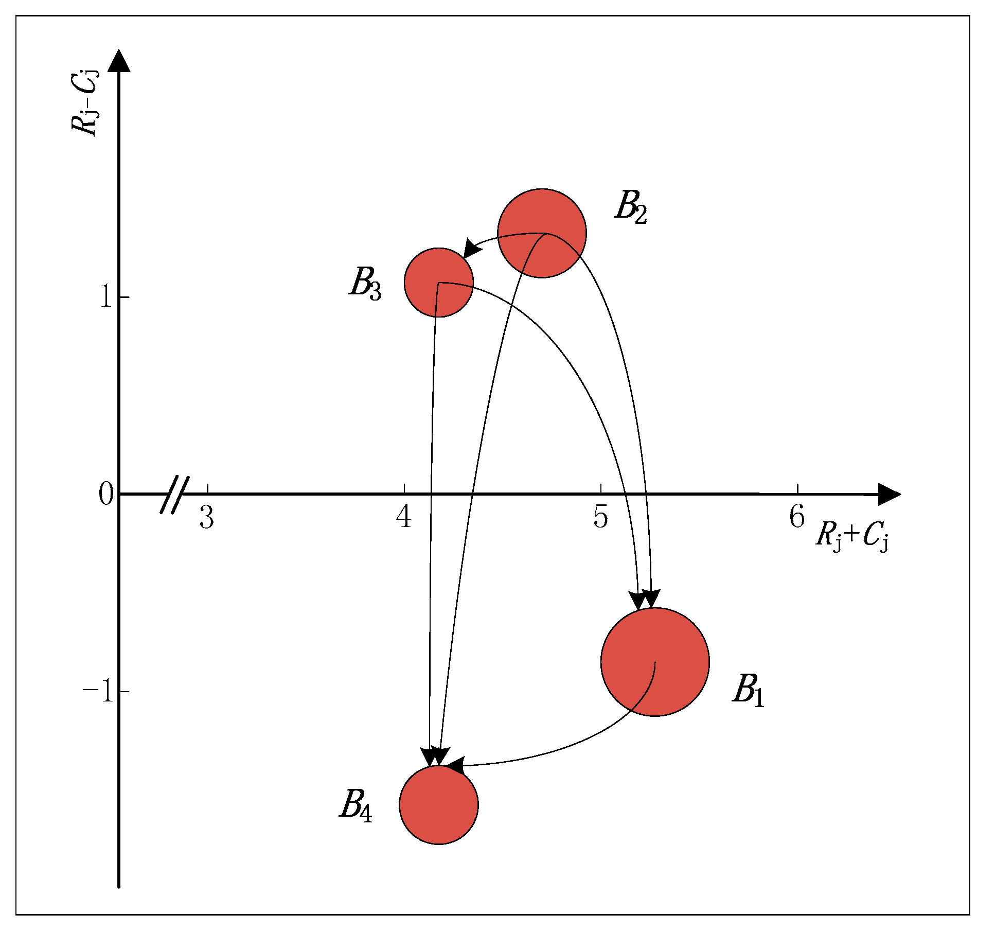
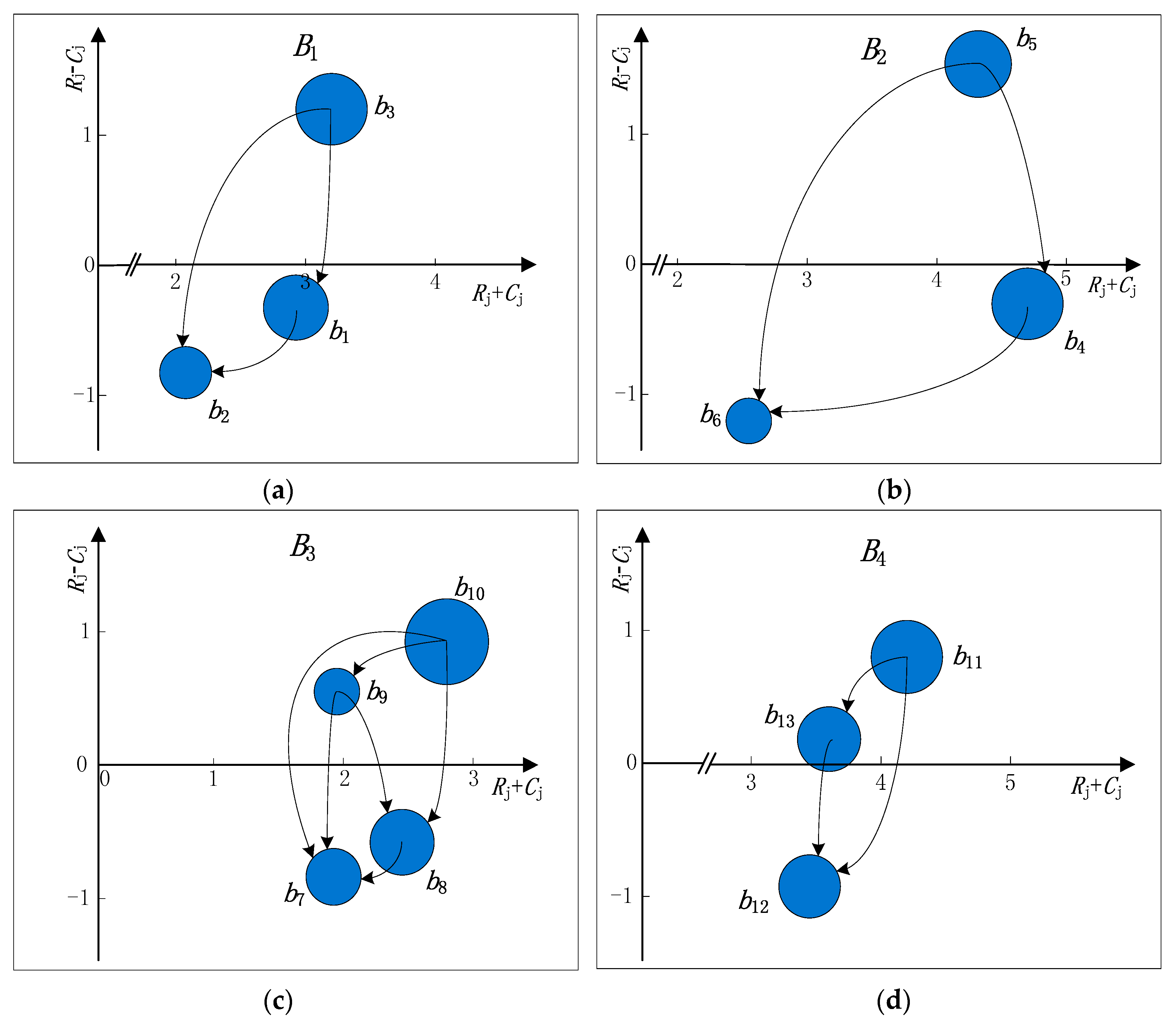
In order to get a causal diagram, the values of and are calculated. The causal diagram can be obtained by mapping in coordinates, where the horizontal axis is called “prominence” and the vertical axis is called “net effect”. In the causal diagram, the prominence axis shows the relative importance of each attribute in the attributes set, and the net effect axis divides the attributes set into cause and effect groups. When , it means that the attribute belongs to the cause group and that it is a net causer; when , it means that the attribute belongs to the effect group and that it is a net receiver. Hence, the complex causalities between attributes could be revealed by the structural correlation coefficients and visualized in the obtained causal diagram.
Step 6: Calculate the hierarchical attribute weights.
In this step, we use the structural correlation coefficients to set the attribute weights that will be used in the decision process. The weight
of attribute
is calculated as follows:
The weight
of attribute
can be normalized as follows:
So the normalized attribute weight vector
can be obtained. Similarly, the sub-attribute weight vector
can also be calculated, and then the overall weight
of the
f-th sub-attribute under the
j-th attribute is defined as follows:
where
is the weight of the
j-th attribute in
, and
is the weight of the
f-th sub-attribute in
.
4.4. The Decision-Making Steps
In summary, the main steps of the proposed decision-making method with grey multi-source heterogeneous data are given as follows:
Step 1: Normalize the comprehensive decision matrix with Equations (1)–(6);
Step 2: Construct the kernel vector and greyness degree vector of grey multi-source heterogeneous data sequence with Equations (7) and (8), then the positive and negative ideal kernel vector as well as the positive and negative ideal greyness degree vector are determined according to Definition 7;
Step 3: Calculate the hierarchical attribute weights with Equations (20)–(26);
Step 4: Calculate the projection values of each alternative on kernel positive and negative ideal alternative as well as greyness degree positive and negative ideal alternative with Equations (9)–15);
Step 5: Calculate the comprehensive optimal membership degree of each alternative with Equations (16)–(19);
Step 6: Rank alternatives. Sorting the values of the comprehensive optimal membership degree in a descending sequence. The larger the value of , the better the preference of the alternative .
5. Case Study
In this section, a case of green supplier selection about product material component is presented based on the proposed method.
5.1. Case Background
With the increasingly serious environmental problems, the green supply chain management (GSCM) has been accepted as a modern management mode. Because green supplier is the upstream of the entire supply chain, its function in cost savings and environmental protection can pass through the supply chain to all downstream links [
50]. It can bring a competitive advantage to the entire supply chain.
Hence, a decision problem of a product material component manufacturer is taken as an example, which aims to select the best green supplier for production. The four potential green suppliers are denoted as
,
,
,
, respectively. We analyze the literature which derives from the literature review of the green supplier selection in
Section 2. Meanwhile, we consult some experts and perform practical investigation in some enterprises. Then a set of green supplier selection attributes are identified. The attributes including the product competitiveness, the enterprise competitiveness and the cooperation support are selected as the primary conventional attributes and the green level is selected as the green attribute. Similarly, we arrive at thirteen sub-attributes. The attributes of the green supplier selection are shown in
Table 1.
In order to evaluate the potential green suppliers objectively and comprehensively, we investigate and obtain the decision information from multiple sources. Meanwhile, owing to the complexity and uncertainty of the actual decision environment, the obtained decision information is usually grey number, and then the fusion of different data types of grey information from multiple sources forms grey multi-source heterogeneous data sequence. The decision information about the four green suppliers are shown in
Table 2, where the data of sub-attributes
(%),
(score),
(score) are obtained from the procurement department and the material controlling department; the data of sub-attributes
(%),
(yuan),
(%) are obtained from the production department and the quality management department; the data of sub-attributes
(score),
(score),
(%),
(score) are obtained from the financial department and the technology department; the data of sub-attributes
(score),
(score),
(%) are obtained from the after-sale service department and the logistics department.
To select the best green supplier for production, the proposed method with grey multi-source heterogeneous data is used to solve the green supplier selection problem. The main rationale is that the kernel and greyness degree which form the common information characteristics of grey multi-source heterogeneous data are utilized to handle the decision information. Considering the multi-attribute multi-level decision structure in green supplier selection, the HG-DEMATEL method is used to capture the causalities between hierarchical attributes and determine the importance of hierarchical attributes. On this basis, the grey relational bi-directional projection method is used to rank the green suppliers, which can measure the proximity and the changing direction between the green suppliers and the positive (negative) ideal solution more accurately.
5.2. The Ranking of Alternatives
Step 1: Normalize the decision information in
Table 2 with Equations (1)–(6), and the normalized comprehensive decision matrix is shown in
Table 3.
Step 2: Construct the kernel vector and greyness degree vector of each alternative with Equations (7) and (8), then kernel matrix organized by kernel vectors and greyness degree matrix organized by greyness degree vectors are constructed, respectively.
Then, the positive and negative ideal kernel vector , as well as the positive and negative ideal greyness degree vector , are determined according to Definition 7.
Step 3: Calculate hierarchical attribute weights.
Firstly, the initial direct relation matrixes
,
, and
that are given by three experts based on an integer scale varying from
are shown in
Table 4.
Secondly, the overall initial direct relation matrix
aggregated by Equation (20) is calculated as follows:
Then, the total relation matrix is calculated by Equation (21);
Finally, the weights of attributes are calculated by Equations (22)–(25) and shown in
Table 5.
Similarly, the normalized weights and overall weights of sub-attributes can be calculated by Equations (20)–(26), and the results are shown in
Table 6.
Step 4: The projection values of each alternative
on kernel positive ideal alternative
and kernel negative ideal alternative
are calculated as follows respectively:
Similarly, the projection values of each alternative
on greyness degree positive ideal alternative
and greyness degree negative ideal alternative
are calculated as follows respectively:
Step 5: Calculate the comprehensive optimal membership degree of each alternative .
The kernel optimal membership degree
and greyness degree optimal membership degree
of each alternative
are calculated as follows respectively:
According to the kernel optimal membership degree
, the ranking result is
, which has a deeper insight into the effect of potentially truly unknown values of grey number on the decision results. According to the greyness degree optimal membership degree
, the ranking result is
, which takes the uncertain extent of grey number into account. Then, we consider the kernel optimal membership degree
and greyness degree optimal membership degree
comprehensively, and the comprehensive optimal membership degree
of each alternative
is calculated as follows respectively:
Step 6: Rank alternatives.
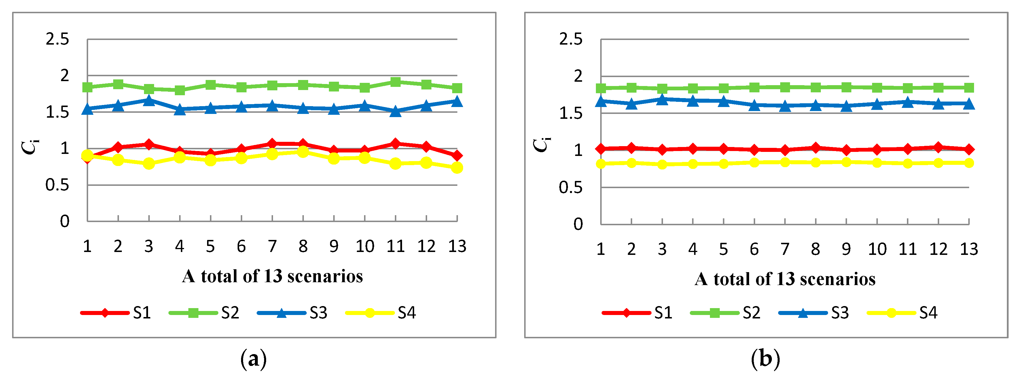
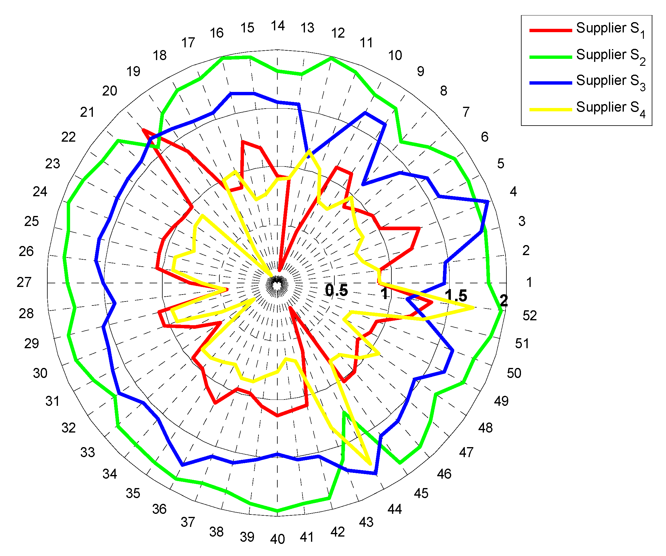
All alternatives are ranked based on the value of each alternative . Sorting the values of in a descending sequence, and final ranking of alternative strategies is obtained as: , that is, the green supplier is the best, and the business decision-makers can give priority to cooperating with the supplier .
5.3. Discussion and Implications
The selection of green supplier is a key step in green supply chain management (GSCM). The proposed decision-making method integrating the HG-DEMATEL and the grey relational bi-directional projection method provides a useful, practical and valid selection tool, which can improve the quality of green supplier selection decisions. We adopt the different data types of grey information from multiple sources to describe the potential green supplier’s comprehensive performance objectively and comprehensively. It is obvious that the decision information from multiple sources can be useful in improving the accuracy of the green supplier selection decisions. Meanwhile, the kernel and greyness degree that are the common information characteristics of grey multi-source heterogeneous data are utilized to process the decision information and avoid the loss of information conversion in green supplier selection effectively.
In making decisions about green supplier selection, the proposed grey relational bi-directional projection method is applied to evaluate the green suppliers. During the evaluation procedure, the distance proximity and the consistency of changing direction between each alternative and the ideal solution are simultaneously taken into consideration, which can more accurately measure the proximity and the similarity between them. By using the proposed method to evaluate and select the potential green suppliers, it can provide a reference value for how to choose the best green supplier to increase the competitiveness and economic level of the company. Moreover, the feasibility and effectiveness of the proposed method are further verified, which also provides some practical and theoretical guidance value for the enterprises that are implementing or will implement green supply chain management.


