2.1. Collection of Data
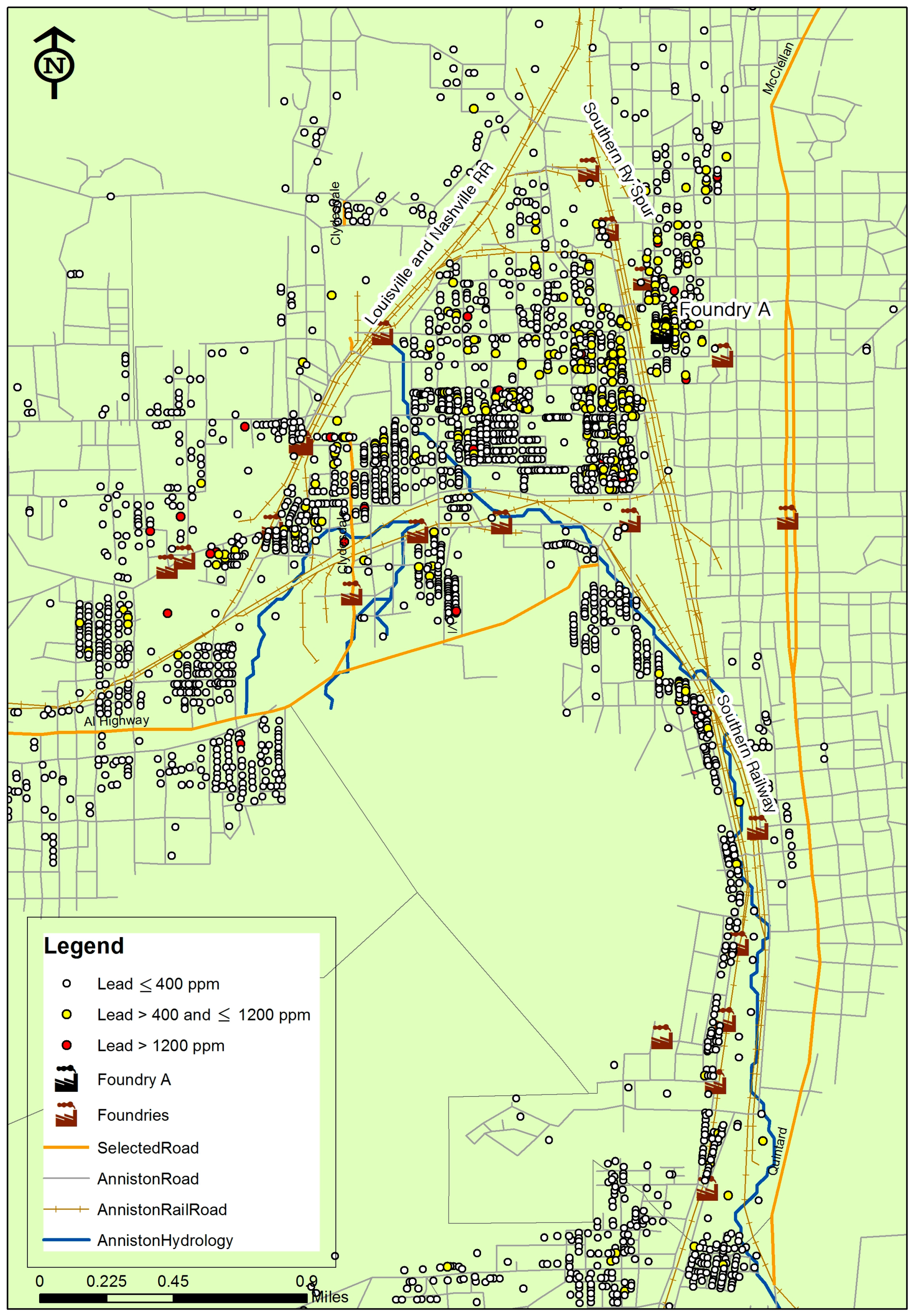
Anniston, Alabama, is located approximately 60 miles east of Birmingham and 90 miles west of Atlanta. It is a community of about 23,000 people and is situated in Calhoun County. The specific areas of interest are residential neighborhoods near 23 former and currently operating foundries, highways, and major railroads in the study area, as shown in
Figure 1. Information on physical variables and soil Pb levels is collected from several data sources. A database of soil samples collected from 2000 to 2008 in Anniston was obtained from the US EPA that includes measurement of Pb levels at 9365 sample locations from residential properties. Multiple lead measurements were taken from the upper 3 inches of soil in each location and reported in parts per million (ppm or mg/kg). Pb levels were measured by US EPA method 3050/6010/6020 (ICP-MS: Inductively coupled plasma-mass spectrometry) [
31]. All soil samples had Pb levels above the matrix specific level of quantification, which ranged from 0.5 to 7 ppm.
The latitude and longitude coordinates contained in the database are used to convert the database into a spatial database. To produce a reliable analysis of lead concentrations, the average concentration is computed for each residential property. This process results in averaged soil lead levels at a total of 2717 residential properties.
Two data sources, Digital Elevation Model (DEM) and Soil Survey Geographic Database (SSURGO), are used to extract some of the physical variables shown in
Table 1. Our initial choice of physical variables included those related to distance from 23 foundries within the study region, distance from roads (highways), distance from railroads, distance from ditches, and distance from each stream order, slope, and soil type. Streams are classified in order of first through to ninth; stream order 1 is the smallest of streams and consists of small tributaries while stream order 9 is considered a river. Slope position is divided into six categories; position 1 indicates locations high on the slope, and position 6 indicates locations near the bottom of the slope. All distance measurements are in meters and fourteen soil texture types are summarized in
Table 1. Soil type is also classified into runoff categories (high, medium and low), into three soil hydrology classes (B: silt loam, C: sandy clay loam, D: clay loam) and into four drainage categories (well, somewhat well, moderate, poor). The final merged dataset that is prepared for further regression analyses contained values of these physical variables for soil sample locations.
Because we are also interested in the socioeconomic and demographic characteristics of the residents living in areas with higher soil lead concentrations, socioeconomic and demographic profiles are extracted from the US EPA and US Bureau of the Census 2010 census block (smallest geographic unit used by the US Census) and block group (a geographic unit between the Census Tract and the Census Block) level data as shown in
Table 2. The Census dataset provides population counts and percentages by race, gender, age, household family, housing unit, education, and income for each of the 4358 census blocks and 87 census-block groups that had recorded populations and percentages. Age is collapsed into the following seven age groups; 0–9, 10–19, 20–29, 30–39, 40–49, 50–64 and 65+. Education level is divided into four categories: no education, elementary school education, high school education, and college or graduate school education. Similarly, the Census dataset includes household family characteristics (average household size, average family size and percent family household), housing unit (occupied housing unit, renter occupied housing unit, housing units built before 1970 and others), employment (labor force and employed labor force), and income (median income and poverty level). We then determine which census block or block-group each soil sample belonged to and then assigned its socioeconomic and demographic profiles to the soil sample for further regression analyses.
2.2. Regression Analyses
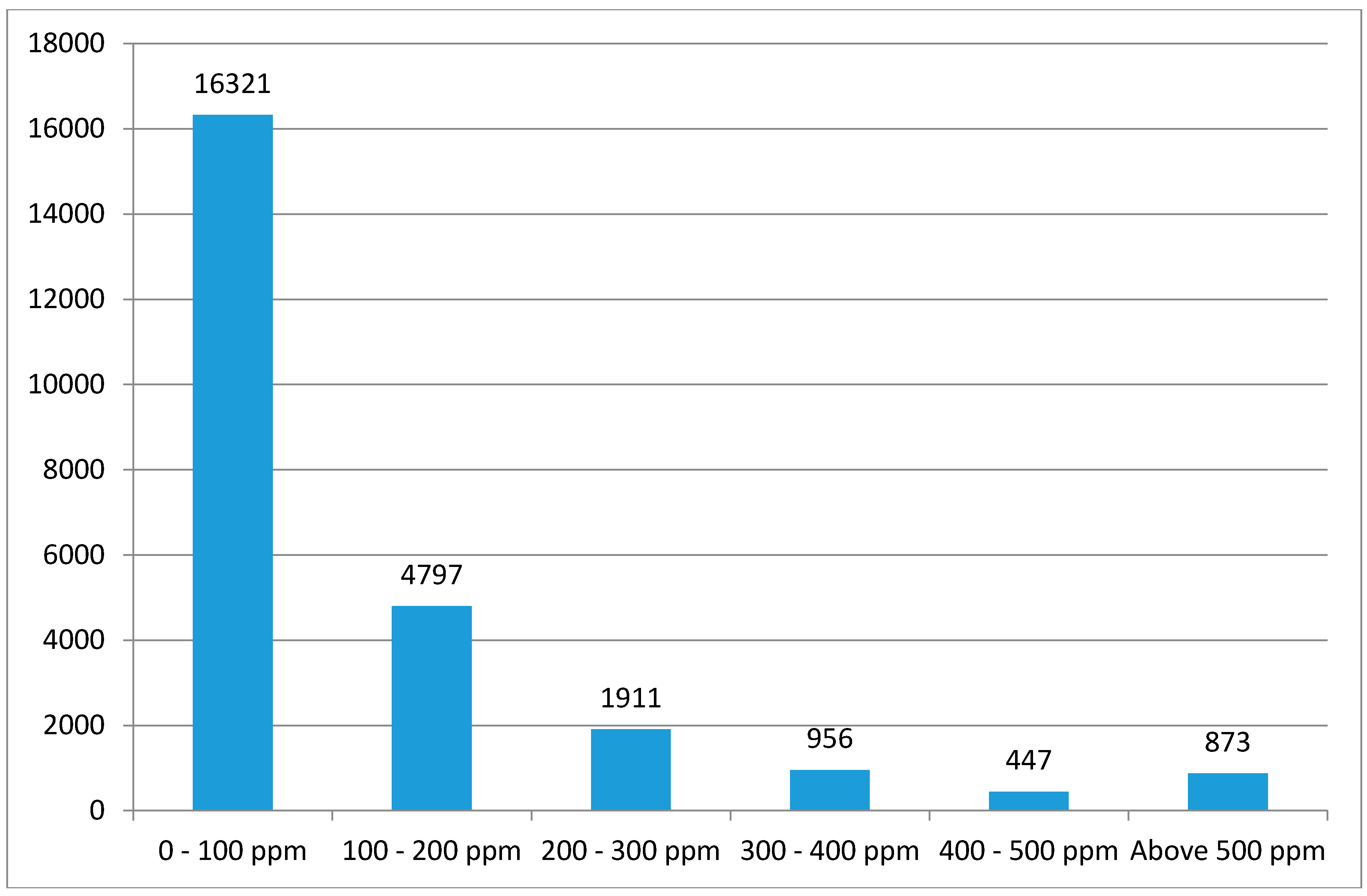
Pollution hazard intensity is modelled at the individual soil lead sample through linear regression on physical and socioeconomic profiles identified during the review of the literature. Ordinary least squares (OLS) stepwise regressions are estimated to find independent variables that are statistically significant in each model at the 0.05 significance level for entry and 0.10 for removal. Results are further checked for multicollinearity based on the variance inflation factor (VIF), where one of the variables concerned is dropped from further consideration. Because the distribution of lead concentrations is markedly skewed, with many small values and a small number of large values as shown in
Figure 2, we use a logarithmic transformation of concentration as the dependent variable. Hence our initial equation is:
where lead is the observed concentration in mg/kg, and the
x’s represent independent variables, while the
b’s represent coefficients for each independent variable.
Given the spatial nature of the data, spatial autocorrelation and heteroscedasticity need to be tested since the residuals and the dependent variables may exhibit not only spatial dependencies but also non-constant error variance. Spatial dependency is a situation where the error term or the dependent variable at a location is correlated with observations on the dependent variable at other nearby locations. Diagnostics of spatial dependencies in the dependent variable and in the residuals are evaluated in the statistical software GeoDaSpace to account for potential spatial effects that may affect estimation results obtained from OLS regressions [
31,
32,
33]. Specifically, the Lagrange Multiplier (LM) test pertaining to both the spatial lag (LM lag) and spatial error models (LM error) are calculated. If both tests are statistically significant, the robust form of the test is used to determine the appropriate model.
Spatial effects evidenced by autocorrelation can be handled econometrically in two primary ways. The spatial lag model includes a spatially lagged dependent variables,
Wy, as one of the explanatory variables:
where
y is a column vector containing the dependent variable;
X is a matrix with a column of ones representing the intercept followed by columns that represent the independent variables,
β is a vector of regression coefficients,
ε is a vector of random error terms, and
ρ is a spatial autoregressive coefficient.
W is a
n ×
n matrix containing zeros on the diagonal; the off-diagonal elements
wij indicate the strength of the relationship between location
i and location
j. In all of the spatial models estimated for this study, the spatial weights matrix is specified using a threshold distance criterion. This is the minimum distance required to ensure that each location has at least one neighbor.
The spatial error model expresses each residual as a function of surrounding residuals. The spatial error model is given by:
where
with the same notation as above and where
λ is an autoregressive regression coefficient, and
Wε captures the spatial lag for errors and the elements of
ξ are normally distributed with mean 1 and variance 1. A spatial error model is estimated by maximum likelihood, while a spatial lag model is best estimated by a two-stage least-squares (2SLS) procedure, which does not assume normality of errors and can accommodate a correction for heteroscedasticity, if present [
32,
33,
34].
A proper regression model is selected by GeoDa’s guidelines [
33]. If the OLS regression exhibits heteroscedasticity only, as shown by the Breusch-Pagan test, then the White correction is applied to the OLS results [
35]. However, if the results of the LM-lag test are significant (or more significant than the LM-error test), then the spatial lag model is carried out as the alternative regression. After the model is run, we apply the Anselin-Keleiian test for residual spatial autocorrelation. If the results of the latter are significant, the model is re-estimated with the heteroskedastic and autocorrelation robust (HAC) approach of Kelejian and Prucha [
35]. In the case where the LM-error test is significant (or more significant than the LM-lag test), then a spatial error model is estimated; in case of heteroscedasticity, the Kelejian-Prucha consistent estimator for heteroscedastic error terms (KP-HET) is used [
34,
36,
37].


