
Local Geographic Variation of Public Services Inequality: Does the Neighborhood Scale Matter?


Abstract
:1. Introduction
- Is it appropriate to use SKATER and SOM models to define the socially meaningful neighborhood? What are their sensitivities, their strengths and limitations in social public service inequality analysis?
- What are the advantages of the GWPCA in measuring inequality in public services within multi-scale neighborhoods compared with the PCA?
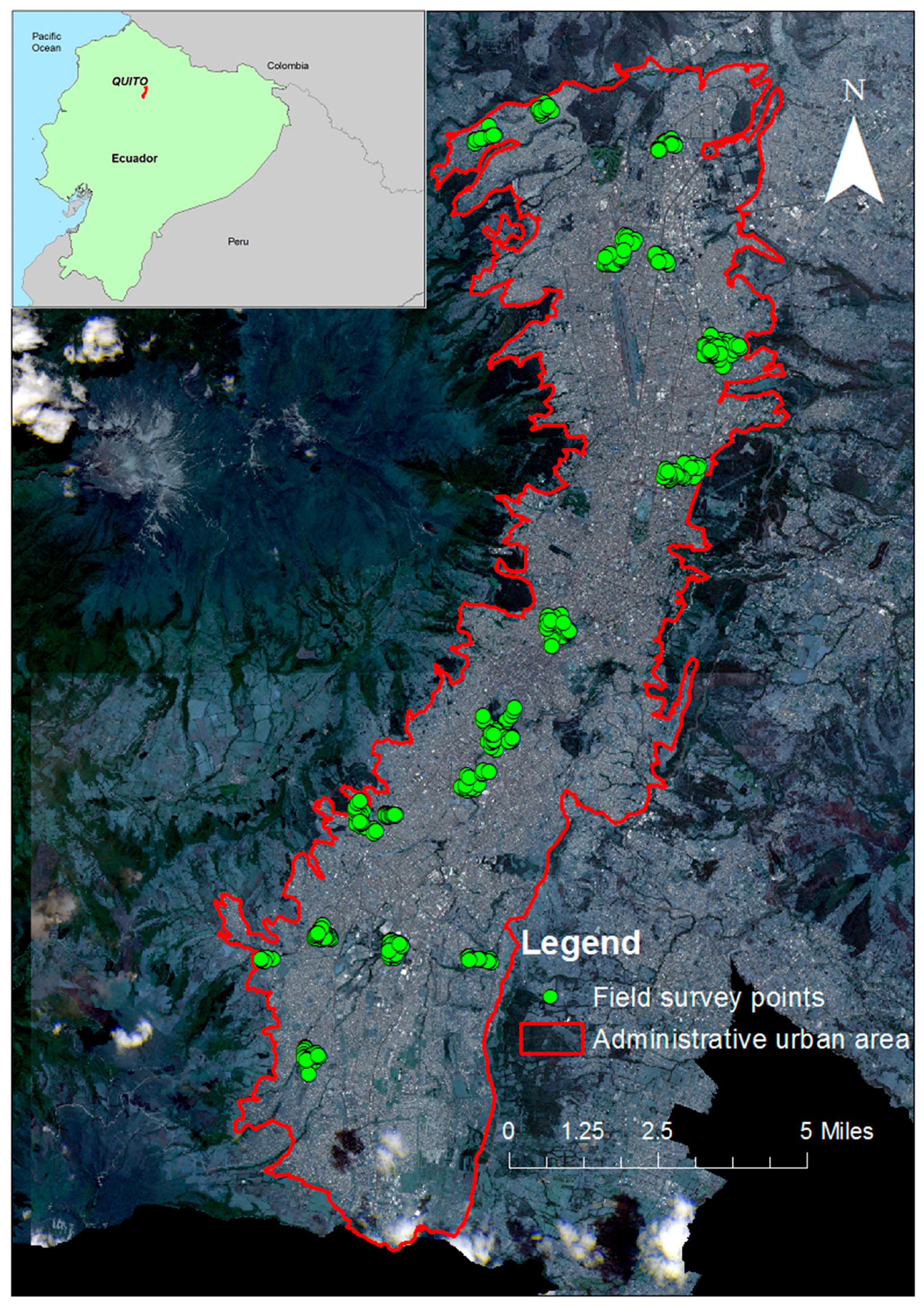
2. Study Area and Data Collection
2.1. Study Area Selection
2.2. Data
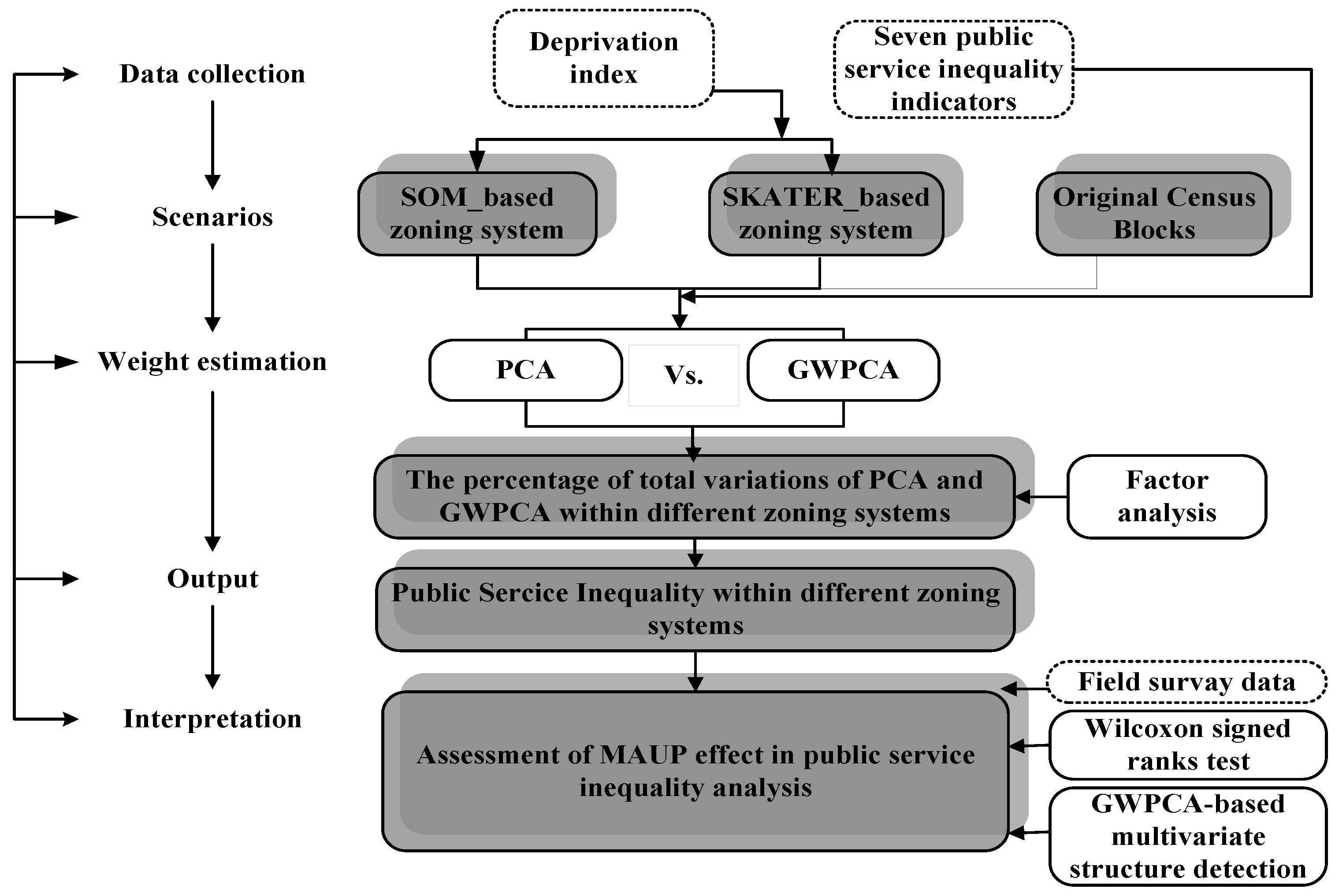
3. Methodology
3.1. Workflow
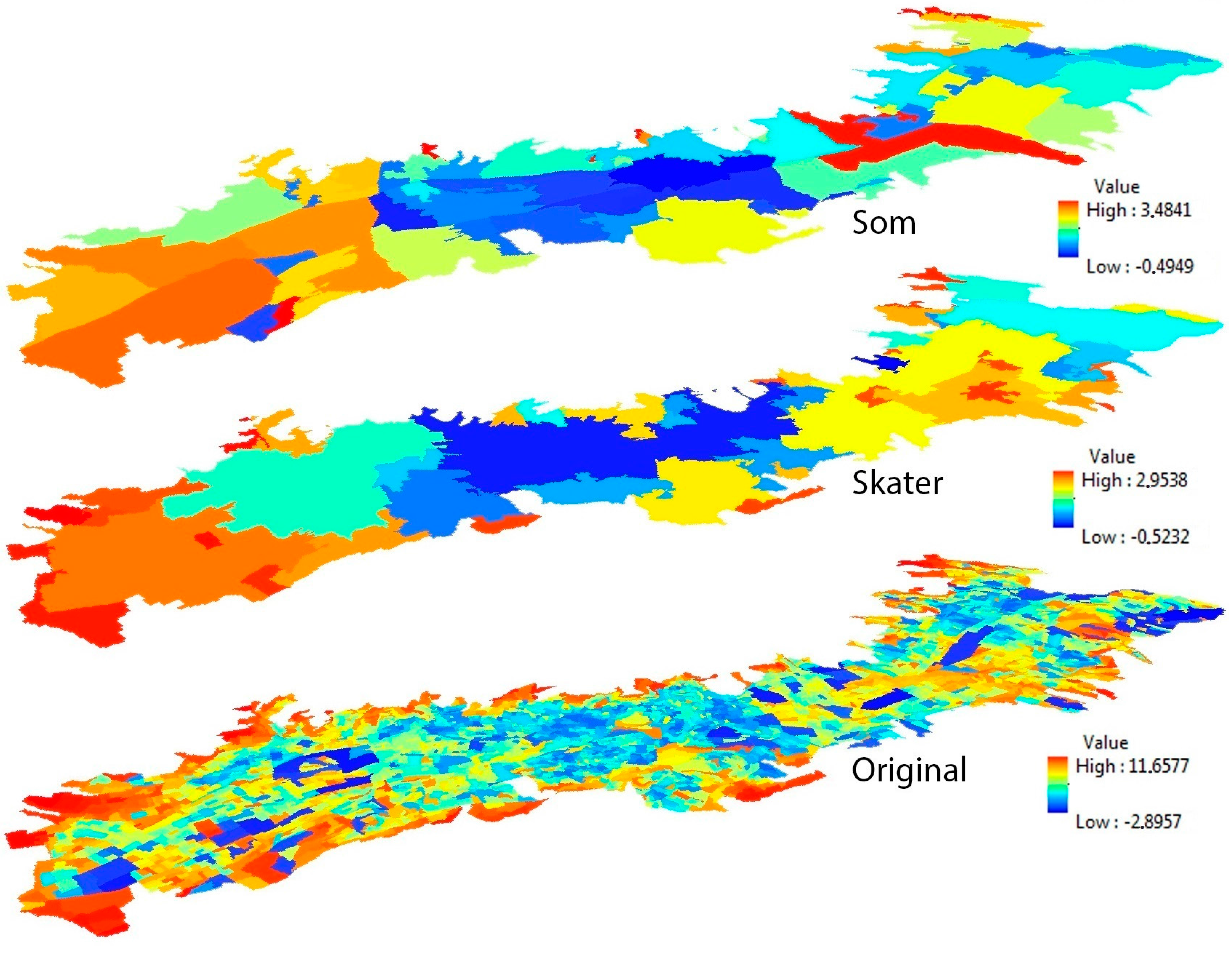
3.2. Urban Regionalization
3.2.1. The Threshold of Urban Regionalization: The Deprivation Index
3.2.2. Self-Organizing Maps (SOM)
3.2.3. Spatial “k”luster Analysis by Tree Edge Removal (SKATER)
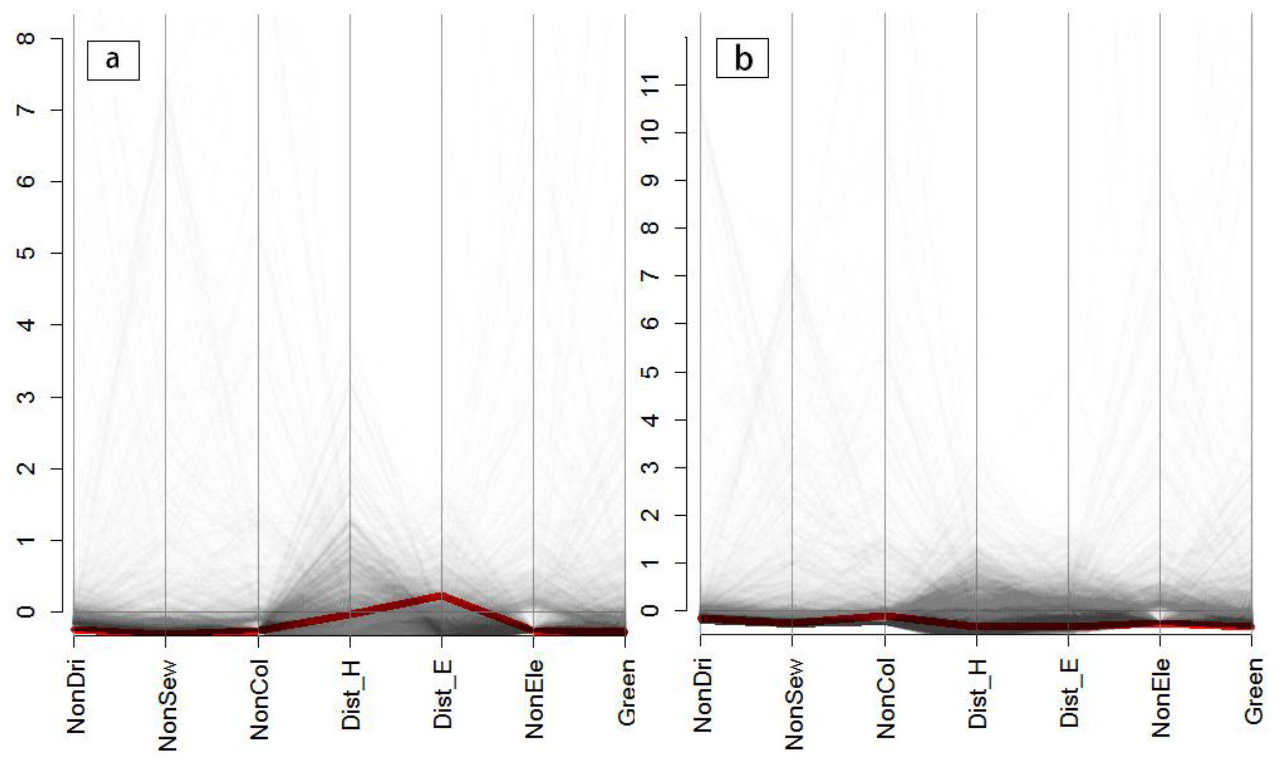
3.3. Public Services Inequality Analysis
3.3.1. Principal Components Analysis
3.3.2. Geographically Weighted Principal Components
3.3.3. Factor Analysis of Public Services Inequalities
3.4. Assessment of MAUP Effects on the Public Service Inequality Analyses
3.4.1. Wilcoxon Signed-Rank Test
3.4.2. The Spatial Heterogeneity of the Set of Public Services Inequality Indicators
4. Results
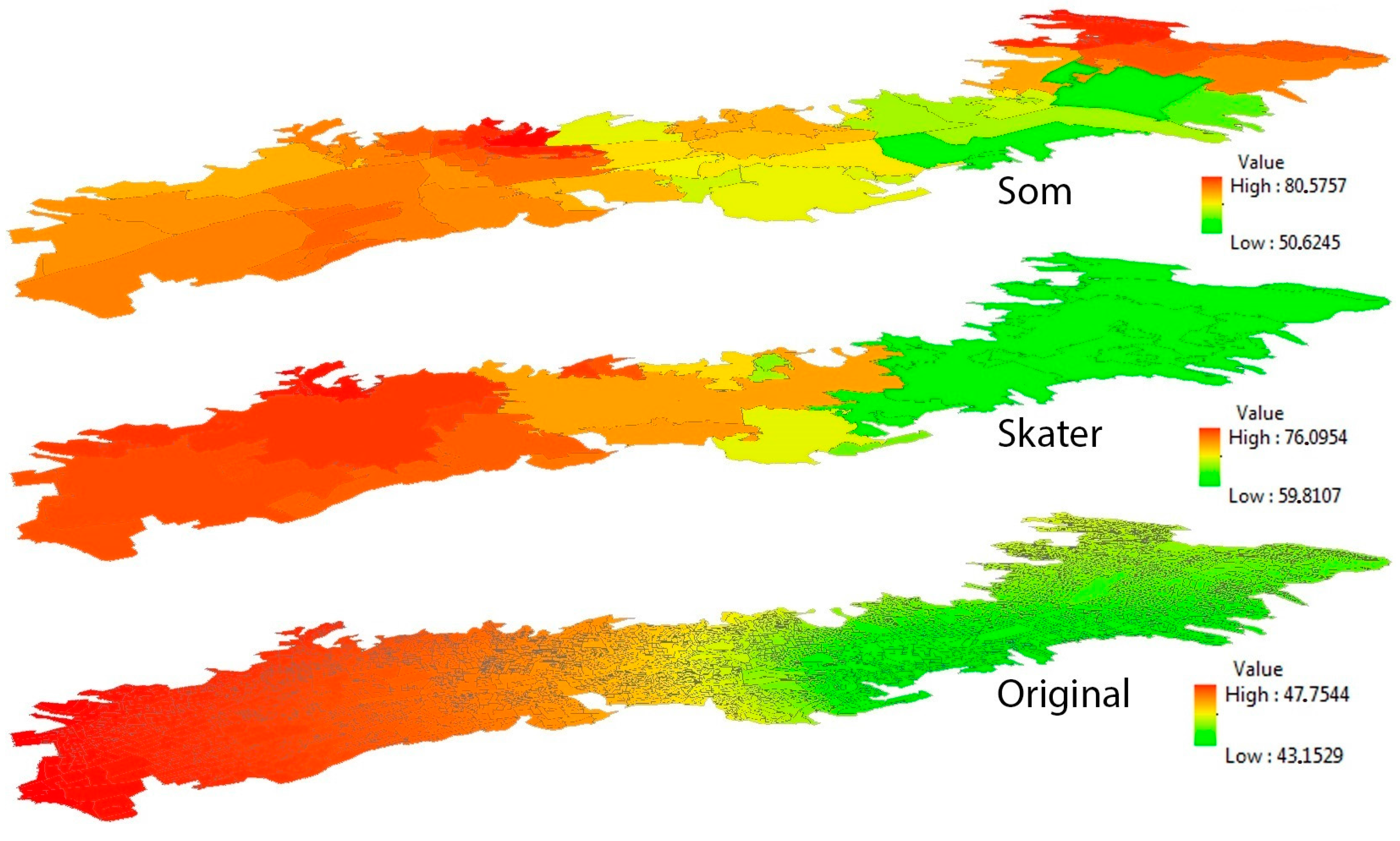
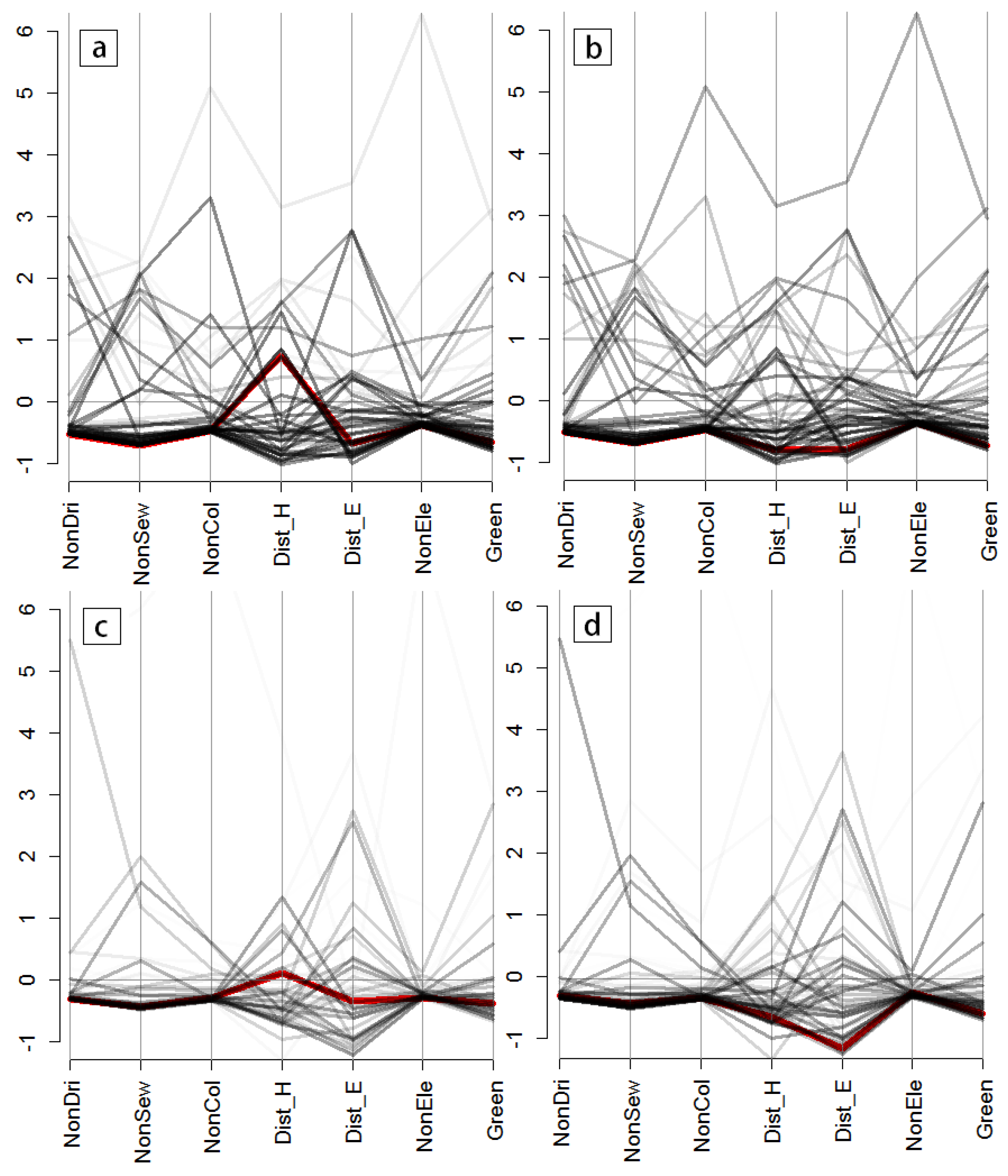
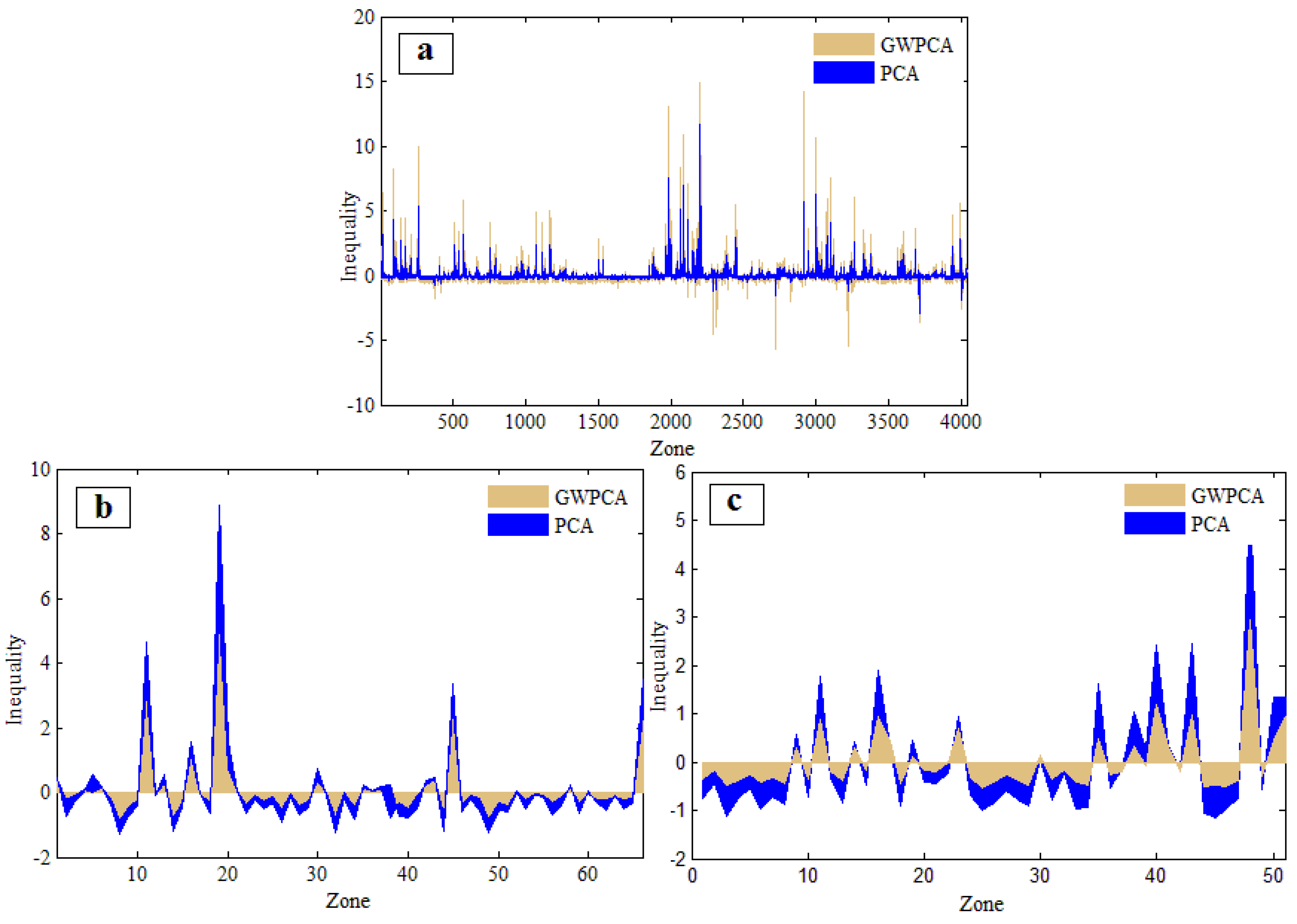
4.1. Visualization of the Variances of Multiple Accessibility Indicators in the Different Zoning Systems
4.2. The Measures of Public Services Inequalities in the Different Zoning Systems
4.3. Assessment of MAUP Effects in the Public Service Inequality Analyses
4.3.1. Wilcoxon Signed-Rank Test
4.3.2. The Spatial Heterogeneity of the Set of Public Services Inequality Indicators
5. Discussion
6. Conclusions
Acknowledgments
Author Contributions
Conflicts of Interest
References
- Baum, F. The New Public Health, 2nd ed.; Oxford University Press: Oxford, UK, 2016; pp. 607–608. [Google Scholar]
- Gostin, L.O.; Gostin, L.O. Public Health Law: Power, Duty, Restraint; University of California Press: Berkeley, CA, USA, 2000; Volume 3, pp. 524–525. [Google Scholar]
- Llewelyn-Davies (Firm); Holden McAllister Partnership. Safer Places: The Planning System and Crime Prevention; Thomas Telford: London, UK, 2004; pp. 48–50. [Google Scholar]
- Newman, J.E.; Clarke, J.H. Publics, Politics and Power: Remaking the Public in Public Services; SAGE Publications Ltd.: Thousand Oaks, CA, USA, 2009; pp. 234–236. [Google Scholar]
- Harvey, B.; Schaefer, A. Managing relationships with environmental stakeholders: A study of UK water and electricity utilities. J. Bus. Ethics 2001, 30, 243–260. [Google Scholar] [CrossRef]
- World Health Organization. Environment and Health Risks: A Review of the Influence and Effects of Social Inequalities. Available online: http://www.euro.who.int/en/health-topics/health-determinants/gender/publications/2010/environment-and-health-risks-a-review-of-the-influence-and-effects-of-social-inequalities (accessed on 1 August 2016).
- Lotfi, S.; Koohsari, M.J. Measuring objective accessibility to neighborhood facilities in the city (A case study: Zone 6 in Tehran, Iran). Cities 2009, 26, 133–140. [Google Scholar] [CrossRef]
- Donkin, A.J.; Dowler, E.A.; Stevenson, S.J.; Turner, S.A. Mapping access to food in a deprived area: The development of price and availability indices. Public Health Nutr. 2000, 3, 31–48. [Google Scholar] [CrossRef] [PubMed]
- Cummins, S.; Macintyre, S. A Systematic study of an urban foodscape: The price and availability of food in Greater Glasgow. Urban Stud. 2002, 39, 2115–2130. [Google Scholar] [CrossRef]
- Apparicio, P.; Cloutier, M.-S.; Shearmur, R. The case of Montréal’s missing food deserts: Evaluation of accessibility to food supermarkets. Int. J. Health Geogr. 2007, 6, 1–6. [Google Scholar] [CrossRef] [PubMed]
- Hillsdon, M.; Panter, J.; Foster, C.; Jones, A. The relationship between access and quality of urban green space with population physical activity. Public Health 2006, 120, 1127–1132. [Google Scholar] [CrossRef] [PubMed]
- Coutts, C. Greenway accessibility and physical-activity behavior. Environ. Plan B Plan. Des. 2008, 35, 552–563. [Google Scholar] [CrossRef]
- Sugiyama, T.; Leslie, E.; Giles-Corti, B.; Owen, N. Associations of neighbourhood greenness with physical and mental health: Do walking, social coherence and local social interaction explain the relationships? J. Epidemiol. Community Health 2008, 62, 9–15. [Google Scholar] [CrossRef]
- Tanser, F.; Gijsbertsen, B.; Herbst, K. Modelling and understanding primary health care accessibility and utilization in rural South Africa: An exploration using a geographical information system. Soc. Sci. Med. 2006, 63, 691–705. [Google Scholar] [CrossRef] [PubMed]
- Law, M.; Wilson, K.; Eyles, J.; Elliott, S.; Jerrett, M.; Moffat, T.; Luginaah, I. Meeting health need, accessing health care: The role of neighbourhood. Health Place 2005, 11, 367–377. [Google Scholar] [CrossRef] [PubMed]
- Cabrera-Barona, P.; Blaschke, T.; Kienberger, S. Explaining Accessibility and Satisfaction Related to Healthcare: A Mixed-Methods Approach. Soc. Indic. Res. 2016, 6, 1–21. [Google Scholar] [CrossRef]
- Luo, W.; Wang, F. Measures of spatial accessibility to health care in a GIS environment: Synthesis and a case study in the Chicago Region. Environ. Plan B Plan. Des. 2003, 30, 865–884. [Google Scholar] [CrossRef]
- Diez, R.; Evenson, K.R.; McGinn, A.P.; Brown, D.G.; Moore, L.; Brines, S.; Jacobs, D.R., Jr. Availability of recreational resources and physical activity in adults. Am. J. Public Health 2007, 97, 493–499. [Google Scholar]
- Cradock, A.L.; Kawachi, I.; Colditz, G.A.; Hannon, C.; Melly, S.J.; Wiecha, J.L.; Gortmaker, S.L. Playground safety and access in Boston neighborhoods. Am. J. Prev. Med. 2005, 28, 357–363. [Google Scholar] [CrossRef] [PubMed]
- Adlakha, D.; Hipp, J.A.; Brownson, R.C. Adaptation and evaluation of the neighborhood environment walkability scale in India (NEWS-India). Int. J. Environ. Res. Public Health 2016, 13, 401–412. [Google Scholar] [CrossRef] [PubMed]
- Long, R.N.; Renne, E.P.; Basu, N. Understanding the social context of the ASGM sector in Ghana: A qualitative description of the demographic, health, and nutritional characteristics of a small-scale gold mining community in Ghana. Int. J. Environ. Res. Public Health 2015, 12, 12679–12696. [Google Scholar] [CrossRef] [PubMed]
- Lopez, R.P.; Hynes, H.P. Obesity, physical activity, and the urban environment: Public health research needs. Environ. Health 2006, 5, 25–30. [Google Scholar] [CrossRef] [PubMed] [Green Version]
- Centers for Disease Control and Prevention (CDC). Neighborhood safety and the prevalence of physical inactivity—Selected states, 1996. MMWR Morb. Mortal. Wkly. Rep. 1999, 48, 143–146. [Google Scholar]
- Tzoulas, K.; Korpela, K.; Venn, S.; Yli-Pelkonen, V.; Kaźmierczak, A.; Niemela, J.; James, P. Promoting ecosystem and human health in urban areas using Green Infrastructure: A literature review. Landsc. Urban Plan. 2007, 81, 167–178. [Google Scholar] [CrossRef]
- Pampel, F.C.; Krueger, P.M.; Denney, J.T. Socioeconomic disparities in health behaviors. Annu. Rev. Sociol. 2010, 36, 349–370. [Google Scholar] [CrossRef] [PubMed]
- Kawachi, I.; Kennedy, B.P. Socioeconomic determinants of health: Health and social cohesion: Why care about income inequality? BMJ 1997, 314, 1037–1040. [Google Scholar] [CrossRef] [PubMed]
- Guo, J.Y.; Bhat, C.R. Operationalizing the concept of neighborhood: Application to residential location choice analysis. J. Transp. Geogr. 2007, 15, 31–45. [Google Scholar] [CrossRef]
- Zenk, S.N.; Schulz, A.J.; Israel, B.A.; James, S.A.; Bao, S.; Wilson, M.L. Neighborhood racial composition, neighborhood poverty, and the spatial accessibility of supermarkets in Metropolitan Detroit. Am. J. Public Health 2005, 95, 660–667. [Google Scholar] [CrossRef] [PubMed]
- Dietz, R.D. The estimation of neighborhood effects in the social sciences: An interdisciplinary approach. Soc. Sci. Res. 2002, 31, 539–575. [Google Scholar] [CrossRef]
- White, A.N. Accessibility and public facility location. Econ. Geogr. 1979, 55, 18–35. [Google Scholar] [CrossRef]
- Saib, M.-S.; Caudeville, J.; Beauchamp, M.; Carré, F.; Ganry, O.; Trugeon, A.; Cicolella, A. Building spatial composite indicators to analyze environmental health inequalities on a regional scale. Environ. Health 2015, 14, 68–80. [Google Scholar] [CrossRef] [PubMed]
- Weiss, L.; Ompad, D.; Galea, S.; Vlahov, D. Defining neighborhood boundaries for urban health research. Am. J. Prev. Med. 2007, 32, 154–159. [Google Scholar] [CrossRef] [PubMed]
- Krieger, N.; Chen, J.T.; Waterman, P.D.; Soobader, M.-J.; Subramanian, S.V.; Carson, R. Choosing area based socioeconomic measures to monitor social inequalities in low birth weight and childhood lead poisoning: The Public Health Disparities Geocoding Project (US). J. Epidemiol. Community Health 2003, 57, 186–199. [Google Scholar] [CrossRef] [PubMed]
- Parliamentary and Health Service Ombudsm. Improving Public Service: A Matter of Principle. Available online: http://www.ombudsman.org.uk/__data/assets/pdf_file/0011/1028/Improving-public-service-a-matter-of-principle.pdf (accessed on 1 August 2016).
- Ryan, P.H.; Brokamp, C.; Fan, Z.-H.; Rao, M.B. Analysis of personal and home characteristics associated with the elemental composition of PM2.5 in indoor, outdoor, and personal air in the RIOPA study. Res. Rep. Health Eff. Inst. 2015, 185, 3–40. [Google Scholar] [PubMed]
- Wang, Z.; Dang, S.; Xing, Y.; Li, Q.; Yan, H. Applying rank sum ratio (RSR) to the evaluation of feeding practices behaviors, and its associations with infant health risk in Rural Lhasa, Tibet. Int. J. Environ. Res. Public Health 2015, 12, 15173–15181. [Google Scholar] [CrossRef] [PubMed]
- Van de Glind, I.; Berben, S.; Zeegers, F.; Poppen, H.; Hoogeveen, M.; Bolt, I.; van Grunsven, P.; Vloet, L. A national research agenda for pre-hospital emergency medical services in The Netherlands: A Delphi-study. Scand. J. Trauma Resusc. Emerg. Med. 2016, 24, 2016. [Google Scholar] [CrossRef] [PubMed]
- Gao, Y.; Gao, J.; Chen, J.; Xu, Y.; Zhao, J. Regionalizing aquatic ecosystems based on the river subbasin taxonomy concept and spatial clustering techniques. Int. J. Environ. Res. Public Health 2011, 8, 4367–4385. [Google Scholar] [CrossRef] [PubMed]
- Hosking, J.R.M.; Wallis, J.R. Some statistics useful in regional frequency analysis. Water Resour. Res. 1993, 29, 271–281. [Google Scholar] [CrossRef]
- Brunsdon, C.; Fotheringham, A.S.; Charlton, M. Spatial nonstationarity and autoregressive models. Environ. Plan. A 1998, 30, 957–973. [Google Scholar] [CrossRef]
- Brunsdon, C.; Fotheringham, S.; Charlton, M. Geographically weighted regression-modelling spatial non-stationarity. J. R. Stat. Soc. Ser. Stat. 1998, 47, 431–443. [Google Scholar] [CrossRef]
- Harris, P.; Brunsdon, C.; Charlton, M. Geographically weighted principal components analysis. Int. J. Geogr. Inf. Sci. 2011, 25, 1717–1736. [Google Scholar] [CrossRef]
- Cleak, H. Health inequality: An introduction to theories, concepts and methods. Aust. Soc. Work 2005, 58, 326–327. [Google Scholar] [CrossRef]
- Manor, O.; Matthews, S.; Power, C. Comparing measures of health inequality. Soc. Sci. Med. 1997, 45, 761–771. [Google Scholar] [CrossRef]
- Kakwani, N.; Wagstaff, A.; van Doorslaer, E. Socioeconomic inequalities in health: Measurement, computation, and statistical inference. J. Econom. 1997, 77, 87–103. [Google Scholar] [CrossRef]
- Fiscella, K.; Franks, P.; Gold, M.R.; Clancy, C.M. Inequality in quality: Addressing socioeconomic, racial, and ethnic disparities in health care. JAMA 2000, 283, 2579–2584. [Google Scholar] [CrossRef] [PubMed]
- Costa, G.; Marinacci, C.; Caiazzo, A.; Spadea, T. Individual and contextual determinants of inequalities in health: The Italian case. Int. J. Health Serv. 2003, 33, 635–667. [Google Scholar] [CrossRef] [PubMed]
- Gordon-Larsen, P.; Nelson, M.C.; Page, P.; Popkin, B.M. Inequality in the built environment underlies key health disparities in physical activity and obesity. Pediatrics 2006, 117, 417–424. [Google Scholar] [CrossRef] [PubMed]
- Pickett, K.E.; Pearl, M. Multilevel analyses of neighbourhood socioeconomic context and health outcomes: A critical review. J. Epidemiol. Community Health 2001, 55, 111–122. [Google Scholar] [CrossRef] [PubMed]
- Haynes, R.; Daras, K.; Reading, R.; Jones, A. Modifiable neighbourhood units, zone design and residents’ perceptions. Health Place 2007, 13, 812–825. [Google Scholar] [CrossRef] [PubMed]
- Fang, J.; Madhavan, S.; Bosworth, W.; Alderman, M.H. Residential segregation and mortality in New York City. Soc. Sci. Med. 1998, 47, 469–476. [Google Scholar] [CrossRef]
- Leclere, F.B.; Rogers, R.G.; Peters, K. Neighborhood social context and racial differences in women’s heart disease mortality. J. Health Soc. Behav. 1998, 39, 91–107. [Google Scholar] [CrossRef] [PubMed]
- Acevedo-Garcia, D. Zip code-level risk factors for tuberculosis: Neighborhood environment and residential segregation in New Jersey, 1985–1992. Am. J. Public Health 2001, 91, 734–741. [Google Scholar] [PubMed]
- Powell, L.M.; Slater, S.; Chaloupka, F.J.; Harper, D. Availability of physical activity—Related facilities and neighborhood demographic and socioeconomic characteristics: A national study. Am. J. Public Health 2006, 96, 1676–1680. [Google Scholar] [CrossRef] [PubMed]
- Hilber, C.A.L. Neighborhood externality risk and the homeownership status of properties. J. Urban Econ. 2005, 57, 213–241. [Google Scholar] [CrossRef]
- Soobader, M.; LeClere, F.B.; Hadden, W.; Maury, B. Using aggregate geographic data to proxy individual socioeconomic status: Does size matter? Am. J. Public Health 2001, 91, 632–636. [Google Scholar] [PubMed]
- Subramanian, S.V.; Lochner, K.A.; Kawachi, I. Neighborhood differences in social capital: A compositional artifact or a contextual construct? Health Place 2003, 9, 33–44. [Google Scholar] [CrossRef]
- Morenoff, J.D.; Sampson, R.J.; Raudenbush, S.W. Neighborhood inequality, collective efficacy, and the spatial dynamics of urban violence. Criminology 2001, 39, 517–558. [Google Scholar] [CrossRef]
- Openshaw, S. A geographical solution to scale and aggregation problems in region-building, partitioning and spatial modelling. Trans. Inst. Br. Geogr. 1977, 2, 459–472. [Google Scholar] [CrossRef]
- Openshaw, S.; Rao, L. Algorithms for Reengineering 1991 Census Geography. Environ. Plan. A 1995, 27, 425–446. [Google Scholar] [CrossRef] [PubMed]
- Alvanides, S.; Openshaw, S. Zone Design for Planning and Policy Analysis; Springer: Berlin, Germany, 1999; pp. 299–315. [Google Scholar]
- Flowerdew, R.; Manley, D.J.; Sabel, C.E. Neighbourhood effects on health: Does it matter where you draw the boundaries? Soc. Sci. Med. 2008, 66, 1241–1255. [Google Scholar] [CrossRef] [PubMed]
- Martin, D. Extending the automated zoning procedure to reconcile incompatible zoning systems. Int. J. Geogr. Inf. Sci. 2003, 17, 181–196. [Google Scholar] [CrossRef]
- Pickett, K.E.; Ahern, J.E.; Selvin, S.; Abrams, B. Neighborhood socioeconomic status, maternal race and preterm delivery: A case-control study. Ann. Epidemiol. 2002, 12, 410–418. [Google Scholar] [CrossRef]
- Flacke, J.; Schüle, S.A.; Köckler, H.; Bolte, G. Mapping environmental inequalities relevant for health for informing urban planning interventions—A case study in the city of Dortmund, Germany. Int. J. Environ. Res. Public Health 2016, 13, 711. [Google Scholar] [CrossRef] [PubMed]
- Wasserman, C.R.; Shaw, G.M.; Selvin, S.; Gould, J.B.; Syme, S.L. Socioeconomic status, neighborhood social conditions, and neural tube defects. Am. J. Public Health 1998, 88, 1674–1680. [Google Scholar] [CrossRef] [PubMed]
- Cockings, S.; Martin, D. Zone design for environment and health studies using pre-aggregated data. Soc. Sci. Med. 2005, 60, 2729–2742. [Google Scholar] [CrossRef] [PubMed]
- Cabrera-Barona, P.; Wei, C.; Hagenlocher, M. Multiscale evaluation of an urban deprivation index: Implications for quality of life and healthcare accessibility planning. Appl. Geogr. 2016, 70, 1–10. [Google Scholar] [CrossRef]
- Parenteau, M.-P.; Sawada, M.C. The Modifiable Areal unit Problem (MAUP) in the Relationship between Exposure to NO2 and Respiratory Health. Available online: http://citeseerx.ist.psu.edu/viewdoc/download?doi=10.1.1.288.536&rep=rep1&type=pdf (accessed on 1 August 2016).
- Cook, T.; Irwin, M. Aggregation Issues in Neighborhood Research: A Comparison of Several Levels of Census Geography and Resident Defined Neighborhoods; Case Western Reserve University: Cleveland, OH, USA, 2004. [Google Scholar]
- Kim, D.R.; Ali, M.; Sur, D.; Khatib, A.; Wierzba, T.F. Determining Optimal Neighborhood Size for Ecological Studies Using Leave-One-Out cross Validation. Available online: http://www.ncbi.nlm.nih.gov/pmc/articles/PMC3361501/ (accessed on 1 August 2016).
- Kelso, J.A.S. Dynamic Patterns: The Self-organization of Brain and Behavior; MIT Press: Cambridge, MA, USA, 1997; pp. 368–371. [Google Scholar]
- Kohonen, T. The self-organizing map. Proc. IEEE 1990, 78, 1464–1480. [Google Scholar] [CrossRef]
- Arribas-Bel, D.; Nijkamp, P.; Scholten, H. Multidimensional urban sprawl in Europe: A self-organizing map approach. Comput. Environ. Urban Syst. 2011, 35, 263–275. [Google Scholar] [CrossRef]
- Jiang, B. A topological pattern of urban street networks: Universality and peculiarity. Phys. Stat. Mech. Its Appl. 2007, 384, 647–655. [Google Scholar] [CrossRef] [Green Version]
- Portugali, J. Self-Organization and the City; Springer Science & Business Media: Berlin, Germany, 2012; pp. 359–402. [Google Scholar]
- AssunÇão, R.M.; Neves, M.C.; Câmara, G.; Freitas, C.D.C. Efficient regionalization techniques for socio-economic geographical units using minimum spanning trees. Int. J. Geogr. Inf. Sci. 2006, 20, 797–811. [Google Scholar] [CrossRef]
- Huie, S.A.B. The concept of neighborhood in health and mortality research. Sociol. Spectr. 2001, 21, 341–358. [Google Scholar] [CrossRef]
- Hoffman, K.; Centeno, M.A. The lopsided continent: Inequality in Latin America. Annu. Rev. Sociol. 2003, 29, 363–390. [Google Scholar] [CrossRef]
- Cabrera-Barona, P.; Murphy, T.; Kienberger, S.; Blaschke, T. A multi-criteria spatial deprivation index to support health inequality analyses. Int. J. Health Geogr. 2015, 14, 11. [Google Scholar] [CrossRef] [PubMed]
- Schkolnik, S.; Chackiel, J. América Latina : Aspectos Conceptuales de Los Censos del 2000; Naciones Unidas: New York, NY, USA, 1999; pp. 20–60. [Google Scholar]
- Mideros, A. Ecuador: Defining and Measuring Multidimensional Poverty, 2006–2010; Cepal Review: Santiago, Chile, 2012; pp. 10–80. [Google Scholar]
- Lalloué, B.; Monnez, J.-M.; Padilla, C.; Kihal, W.; Le Meur, N.; Zmirou-Navier, D.; Deguen, S. A statistical procedure to create a neighborhood socioeconomic index for health inequalities analysis. Int. J. Equity Health 2013, 12, 21. [Google Scholar] [CrossRef] [PubMed] [Green Version]
- Apparicio, P.; Abdelmajid, M.; Riva, M.; Shearmur, R. Comparing alternative approaches to measuring the geographical accessibility of urban health services: Distance types and aggregation-error issues. Int. J. Health Geogr. 2008, 7, 7. [Google Scholar] [CrossRef] [PubMed] [Green Version]
- De la Fuente, H.; Rojas, C.; Salado, M.J.; Carrasco, J.A.; Neutens, T. Socio-Spatial inequality in education facilities in the concepcion Metropolitan Area (Chile). Curr. Urban Stud. 2013, 1, 117–129. [Google Scholar] [CrossRef]
- Guagliardo, M.F. Spatial accessibility of primary care: Concepts, methods and challenges. Int. J. Health Geogr. 2004, 3, 3. [Google Scholar] [CrossRef] [PubMed] [Green Version]
- Jones, S.G.; Ashby, A.J.; Momin, S.R.; Naidoo, A. Spatial implications associated with using Euclidean distance measurements and geographic centroid imputation in health care research. Health Serv. Res. 2010, 45, 316–327. [Google Scholar] [CrossRef] [PubMed]
- Phibbs, C.S.; Luft, H.S. Correlation of travel time on roads versus straight line distance. Med. Care Res. Rev. 1995, 2, 532–542. [Google Scholar] [CrossRef]
- Ngom, R.; Gosselin, P.; Blais, C. Reduction of disparities in access to green spaces: Their geographic insertion and recreational functions matter. Appl. Geogr. 2016, 66, 35–51. [Google Scholar] [CrossRef]
- Aho, A.V.; Hopcroft, J.E.; Ullman, J. Data Structures and Algorithms, 1st ed.; Addison-Wesley Longman Publishing Co., Inc.: Boston, MA, USA, 1983; pp. 10–30. [Google Scholar]
- Nardo, M.; Saisana, M.; Saltelli, A.; Tarantola, S.; Hoffman, A.; Giovannini, E. Handbook on Constructing Composite Indicators; Organisation for Economic Co-operation and Development: Paris, France, 2005; pp. 89–92. [Google Scholar]
- Jolliffe, I. Principal Component Analysis; John Wiley & Sons, Inc.: Hoboken, NJ, USA, 2002; pp. 80–92. [Google Scholar]
- Harris, P.; Brunsdon, C.; Charlton, M.; Juggins, S.; Clarke, A. Multivariate spatial outlier detection using robust geographically weighted methods. Math. Geosci. 2013, 46, 1–31. [Google Scholar] [CrossRef]
- Gollini, I.; Lu, B.; Charlton, M.; Brunsdon, C.; Harris, P. GWmodel: An R Package for Exploring Spatial Heterogeneity Using Geographically Weighted Models. Available online: https://www.jstatsoft.org/article/view/v063i17 (accessed on 1 August 2016).
- Nicoletti, G.; Scarpetta, S.; Boylaud, O. Summary indicators of product market regulation with an extension to employment protection legislation. Available online: http://papers.ssrn.com/sol3/papers.cfm?abstract_id=201668 (accessed on 1 August 2016).
- Woolson, R.F. Wilcoxon signed-rank test. In Wiley Encyclopedia of Clinical Trials; Medical University of South Carolina: Charleston, SC, USA, 2008; pp. 20–25. [Google Scholar]


| Indicators (Ratios) | Variables | Sign a |
|---|---|---|
| No Access to Drinking Water (NonDri) | Number of Households without Access to the Public System of Drinking Water; Total Household Number | + |
| No Access to Sewerage System (NonSew) | Number of Households without Access to the Sewerage System; Total Household Number | + |
| No Access to the Public Electricity Grid (NonEle) | Number of Households without Access to the Public Electricity Grid; Total Household Number | + |
| No Access to Garbage Collection Service (NonCol) | Number of Households without Service of Garbage Collection; Total Household Number | + |
| Limited Access to Health Care Services (Dist_H) | Distance to the nearest Healthcare Service | + |
| Limited Access to Educational Services (Dist_E) | Distance to the nearest Educational Service | + |
| Limited Access to Green Areas (Green) | Ratio of Greenspace in an Area Unit | − |
| Zoning System | Number | HS | NC | NS | QoL |
|---|---|---|---|---|---|
| Census Blocks (GWPCA_PSI) | 142 | 0.059 * | 0.012 | 0.000 | 0.000 |
| Census Blocks (PCA_PSI) | 142 | 0.000 | 0.633 * | 0.000 | 0.000 |
| SOM (GWPCA_PSI) | 19 | 0.003 | 0.821 * | 0.134 * | 0.003 |
| SOM (PCA_PSI) | 19 | 0.001 | 0.512 * | 0.014 | 0.001 |
| SKATER (GWPCA_PSI) | 14 | 0.058 * | 0.065 * | 0.714* | 0.058 * |
| SKATER (PCA_PSI) | 14 | 0.001 | 0.627 * | 0.013 | 0.001 |
© 2016 by the authors; licensee MDPI, Basel, Switzerland. This article is an open access article distributed under the terms and conditions of the Creative Commons Attribution (CC-BY) license (http://creativecommons.org/licenses/by/4.0/).
Share and Cite
Wei, C.; Cabrera-Barona, P.; Blaschke, T. Local Geographic Variation of Public Services Inequality: Does the Neighborhood Scale Matter? Int. J. Environ. Res. Public Health 2016, 13, 981. https://doi.org/10.3390/ijerph13100981
Wei C, Cabrera-Barona P, Blaschke T. Local Geographic Variation of Public Services Inequality: Does the Neighborhood Scale Matter? International Journal of Environmental Research and Public Health. 2016; 13(10):981. https://doi.org/10.3390/ijerph13100981
Chicago/Turabian StyleWei, Chunzhu, Pablo Cabrera-Barona, and Thomas Blaschke. 2016. "Local Geographic Variation of Public Services Inequality: Does the Neighborhood Scale Matter?" International Journal of Environmental Research and Public Health 13, no. 10: 981. https://doi.org/10.3390/ijerph13100981