To assess the impact from the additional parameters (on-road component and indoor infiltration) on STOK, we present our data considering one parameter at a time in each of the first three sub-sections below. In
Section 3.2 and
Section 3.3, we summarize the potential exposure error at population and individual level. Given the multiple models and pollutants discussed below, we have underscored the phrases:
outdoor STOK,
outdoor on-road,
outdoor hybrid,
indoor STOK,
indoor on-road and
indoor hybrid, and italicized the statistical indicators (
spatial CV,
temporal CV,
ND, and
NAD) and the pollutant names (
CO,
NOx,
PM2.5 and
EC) throughout this section, for ease of readability.
3.1. The Effect of on-Road Component
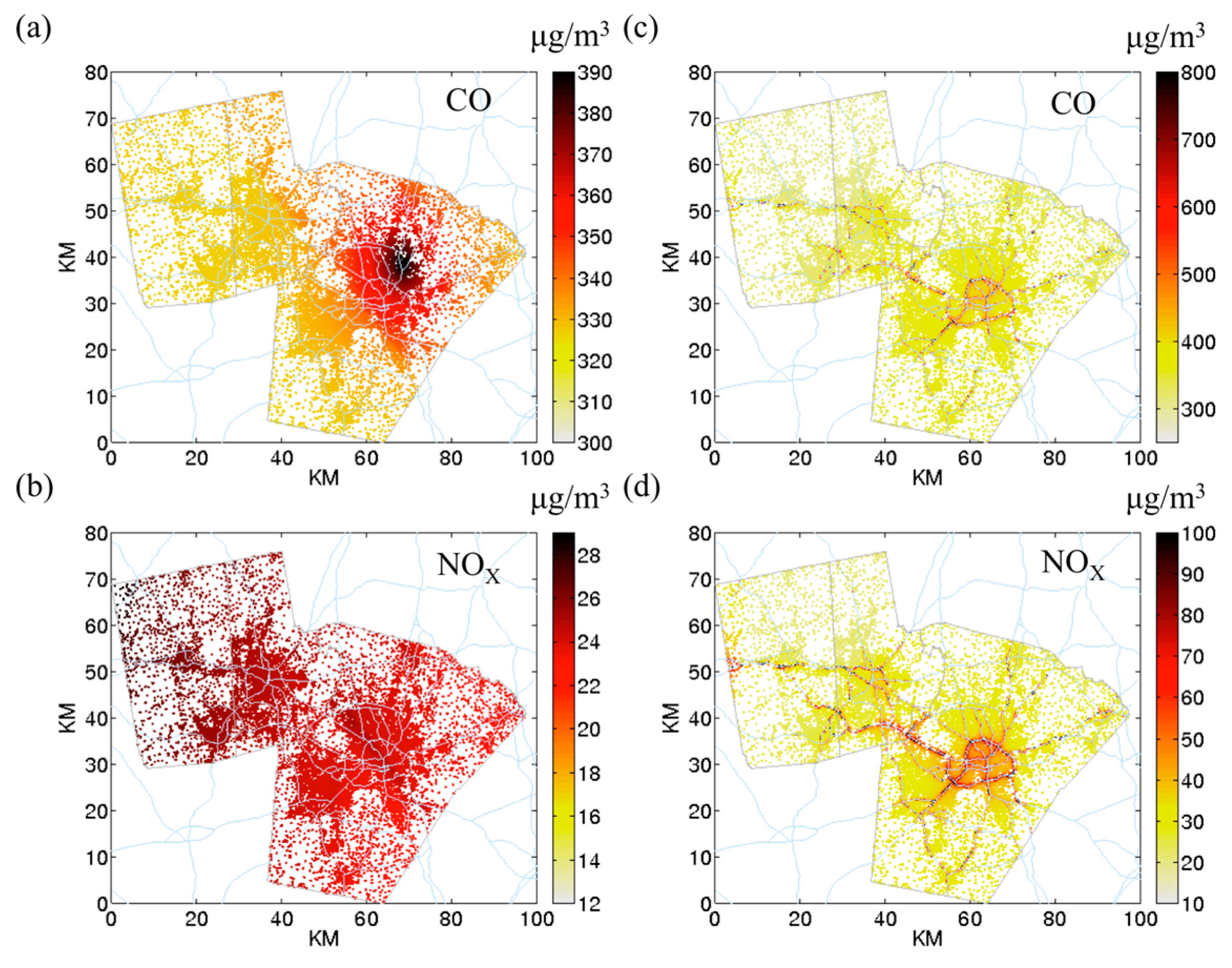
Figure 1 shows the
outdoor STOK and
outdoor hybrid concentration maps for
CO (
Figure 1a,c) and
NOx (
Figure 1b,d) at Census block centroids for four different metrics. We presented morning traffic peak hour (07:00) because the on-road contribution is the greatest. At 07:00, concentration from roadways is clearly seen with
outdoor hybrid (
Figure 1c,d) but not
outdoor STOK (
Figure 1a,b). Note the color scale is different among the four figures to properly display the data. STOK cannot capture the near road concentrations because there is a limited amount of available monitors in this region. Further, the location of monitors is crucial for STOK to estimate the concentration.
CO has a “kriging island” (
i.e., a concentration hotspot surrounding a monitor,
Figure 1a) but not for
NOx (
Figure 1b).
Figure 1.
Outdoor concentration of CO and NOx at Census block centroids at 07:00. (a) CO outdoor space-time ordinary kriging (STOK); (b) NOx outdoor STOK; (c) CO outdoor hybrid; (d) NOx outdoor hybrid. The color bar represents concentration in μg/m3. (Note that the color scale is different for the four figures to emphasize the concentration ranges that vary by pollutant).
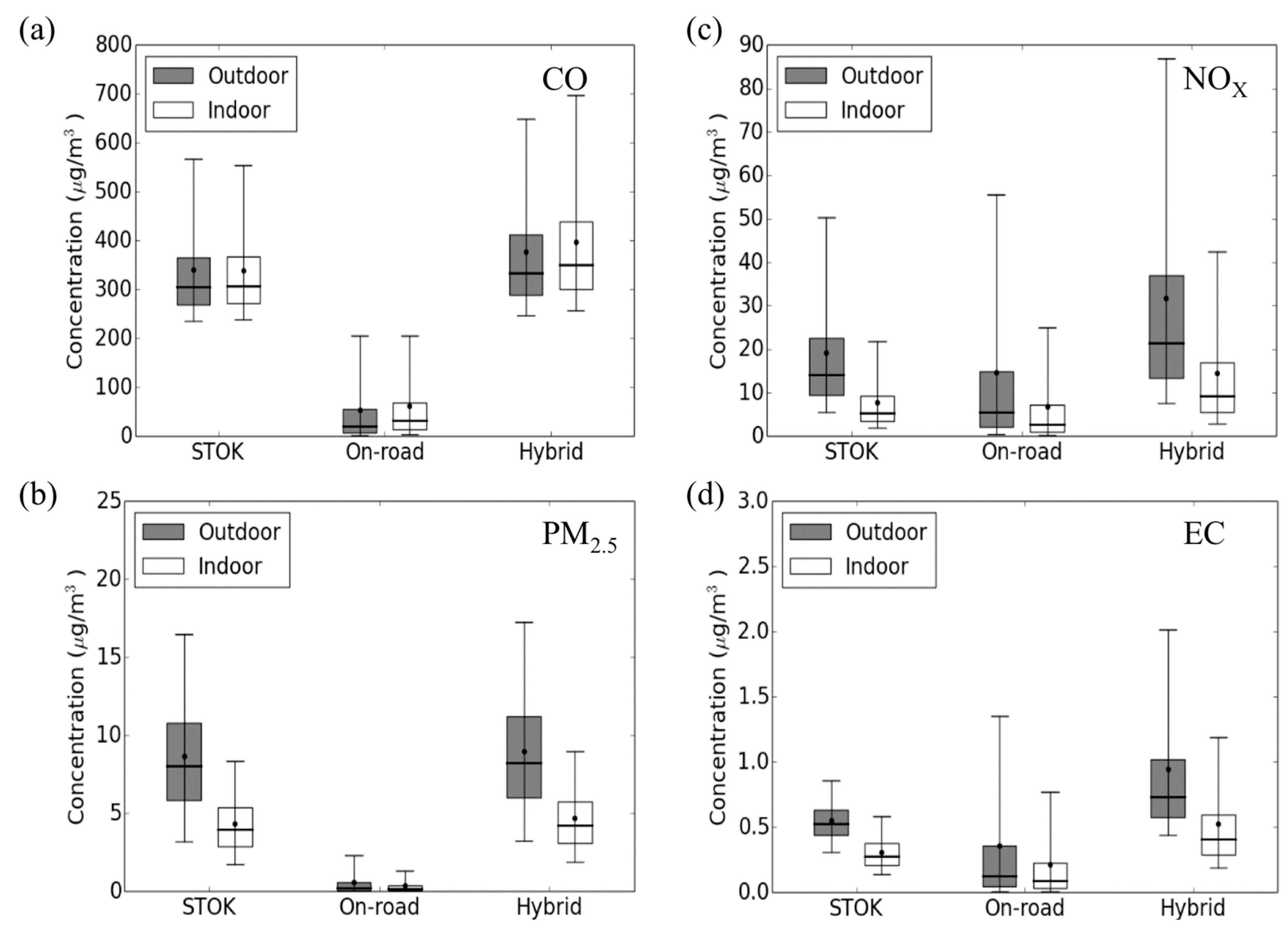
Figure 2 shows the hourly concentration boxplot for the four pollutants under different exposure metrics. For outdoor
CO and
PM2.5, the major contributor to the
outdoor hybrid is the
outdoor STOK. For
CO (
Figure 2a), the average
outdoor STOK (340.45 μg/m
3) is 6.23 times higher than the average
outdoor on-road (54.67 μg/m
3). For
PM2.5 (
Figure 2b), the average
outdoor STOK (8.69 μg/m
3) is 14.02 times higher than the average
outdoor on-road (0.62 μg/m
3). For these two pollutants, because the
outdoor STOK dominates the hybrid concentration, the
outdoor hybrid is less different from the
outdoor STOK concentration.
For
NOx and
EC, both
outdoor STOK and
outdoor on-road contribute significantly to the
outdoor hybrid. For
NOx (
Figure 2c), although the average
outdoor STOK (19.24 μg/m
3) is 32% higher than the
outdoor on-road (14.63 μg/m
3), the upper 95% bound of
outdoor on-road (55.6 μg/m
3) is 10% higher than the
outdoor STOK (50.33 μg/m
3). For
EC (
Figure 2d), the average
outdoor STOK (0.55 μg/m
3) is 52% higher than the
outdoor on-road (0.36 μg/m
3) but the upper 95% bound of outdoor on-road (1.35 μg/m
3) is 57% higher than the
outdoor STOK (0.86 μg/m
3). As a result, for these two pollutants, the average
outdoor hybrid is 65% and 72% higher than the average
outdoor STOK for
NOx and
EC.
As shown in
Figure 1 and the wider range for the
outdoor hybrid compared to
outdoor STOK in
Figure 2 (dark boxes), adding the
outdoor on-road introduces different spatial variability for different pollutants.
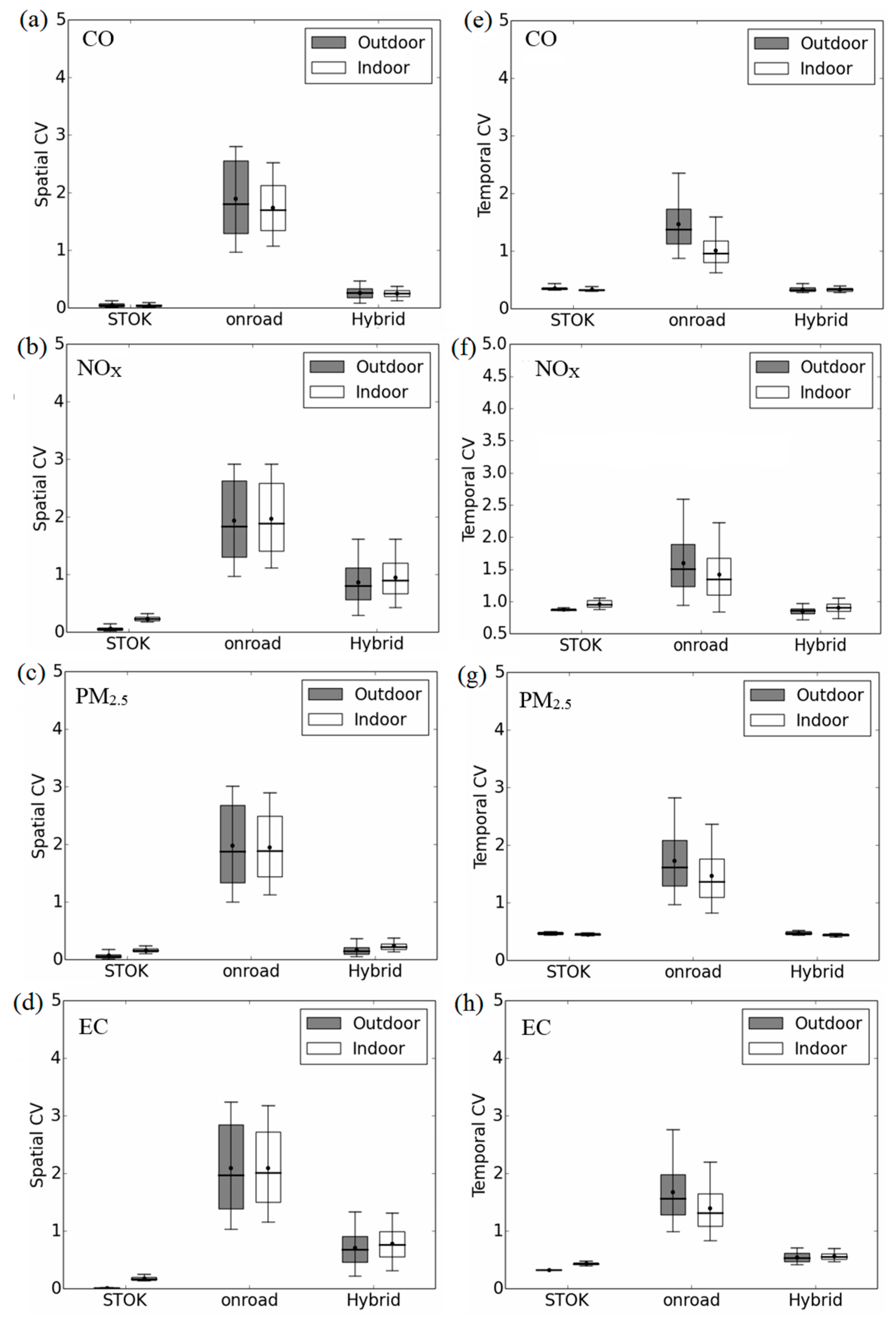
Figure 3 left panel quantifies the spatial component of this variability using
spatial CV. For all pollutants, the
outdoor on-road shows a great spatial variability (average
spatial CV ~2). As a result, for the pollutants that have large contribution from
outdoor on-road concentration (38% for
NOx and 46% for
EC), the
outdoor hybrid would yield much higher spatial variation (average
spatial CV = 0.87 for
NOx and 0.71 for
EC) than
outdoor STOK (average
spatial CV = 0.065 for
NOx (
Figure 3b) and 0.014 for
EC (
Figure 3d)). It is worth noticing that although
CO and
PM2.5 in this region is dominated by background concentration, adding
outdoor on-road can still increase the spatial variability (average
spatial CV from 0.06 for
outdoor STOK to 0.26 for
outdoor hybrid for
CO and 0.07 for
outdoor STOK to 0.17 for
outdoor hybrid for
PM2.5), indicating the importance of the on-road emission for the near-road environment even when the contribution is relatively small (14% for
CO and 7% for
PM2.5). Corroborating illustrations are shown in the authors’ peer-reviewed paper [
39] where the hybrid contribution for
PM2.5 drops by 20% within 150 meters from roadways.
Temporal CV is summarized in
Figure 3 right panel. The
outdoor on-road shows a great temporal variation (average
temporal CV ~1.5, (
Figure 3, dark boxes for
outdoor on-road)). This high temporal variation is from the bottom up approach used in the R-LINE modeling where the temporal pattern of on-road emission is captured. For
CO and
PM2.5 (
Figure 3e,g), the
outdoor hybrid yields similar average
temporal CV to
outdoor STOK because for these two pollutants,
outdoor STOK dominates the total concentration. Therefore, although
outdoor on-road shows large temporal variation, the variation is lost after
outdoor on-road and
outdoor STOK are combined for
CO and
PM2.5. For
NOx (
Figure 3f), although 38% of the
outdoor hybrid is from the
outdoor on-road, because the
outdoor on-road only affects Census blocks within a few hundred meters from roadways, the overall
temporal CV for
outdoor hybrid is less different from the
outdoor STOK. For
EC, because the
outdoor on-road contributes 46% to the
outdoor hybrid, the average
temporal CV increases by 72% from 0.33 for
outdoor STOK to 0.57 for
outdoor hybrid (
Figure 3h).
For the
temporal CV, only the Census blocks near roadways would be affected by
outdoor on-road. Examples for
NOx are shown in
Figure 4 with a Census block that is 14.1 m from a roadway (left panel) and a Census block that is 9.6 km from a roadway (right panel) and comparing concentrations at each of the two locations for a day At the near-road Census block (
Figure 4a),
outdoor on-road contributes, on average, 89% to
outdoor hybrid. The contribution from
outdoor on-road is the greatest (over 90%) during morning (07:00 to 09:00) and afternoon (17:00 to 19:00) traffic peak hours and the
temporal CV increases by 40% (from 0.42 for
outdoor STOK to 0.59 for
outdoor hybrid). On the other hand, at a remote Census block (
Figure 4b), the
outdoor on-road for
NOx contributes, on average, only 18% to the
outdoor hybrid. As a result, the
temporal CV only increases slightly by 7% from 0.44 for
outdoor STOK to 0.47 for
outdoor hybrid. All the other pollutants show a similar pattern as
NOx (
Figure S2).
Figure 2.
Hourly pollutant concentration for each Census block in Durham, Orange, and Wake Counties, North Carolina (NC) in 2012. (a) CO; (b) PM2.5; (c) NOx; and (d) EC. Bottom and top of box represents 25th and 75th percentiles, the line in the middle of the box is the median, the ends of the whisker are the 5th and 95th percentiles, and the dot on the whisker is the mean.
Figure 3.
Spatial CV for each hour (left panel); and Temporal CV for each Census block (right panel) for CO (a,e); NOx (b,f); PM2.5 (c,g); and EC (d,h). Bottom and top of box represents 25th and 75th percentiles, the line in the middle of the box is the median, the ends of the whisker are the 5th and 95th percentiles, and the dot on the whisker is the mean.
Figure 4.
Time series plot on January 3rd for NOx at (a) a near-road Census block (14.1 m from roadway); and (b) a remote Census block (9.6 km from roadway).
Figure 4.
Time series plot on January 3rd for NOx at (a) a near-road Census block (14.1 m from roadway); and (b) a remote Census block (9.6 km from roadway).
The effect of on-road component on indoor metrics shows similar pattern to that of outdoor metrics (White-colored boxes from
Figure 3e,h). We present the difference between outdoor and indoor metrics in the next section.
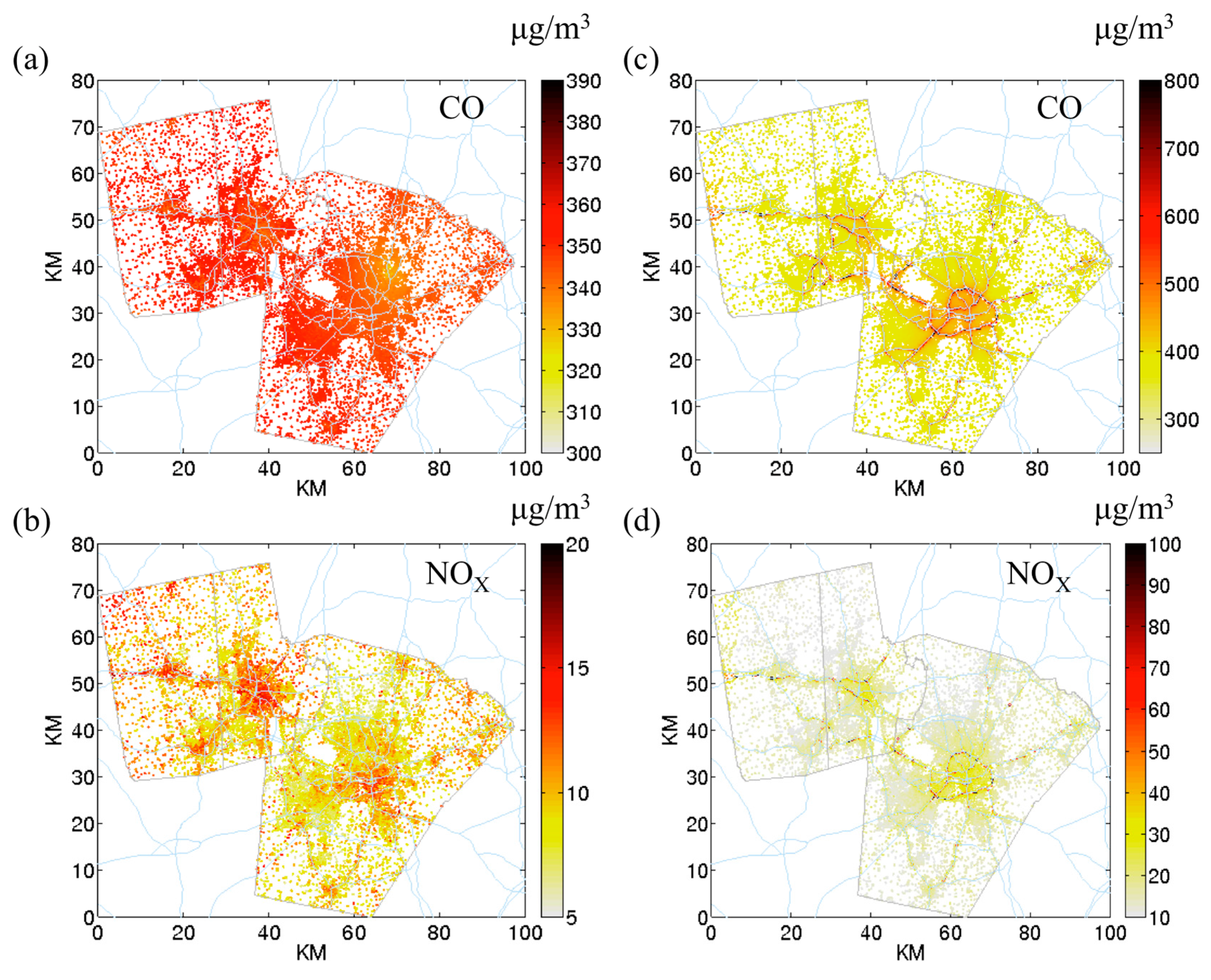
3.2. The Effect of Indoor Infiltration
Figure 5 shows the indoor concentration for
CO and
NOx. At 07:00, the spatial pattern for indoor metrics is similar to the outdoor metrics (
Figure 1) except for
indoor STOK NOx (
Figure 5c). The extra spatial variation for
indoor STOK NOx shows a similar spatial pattern to AER (
Figure S3). However, this pattern is not seen for
CO (
Figure 5a). On average, compared to the outdoor concentration, the indoor concentration is 66% lower for
NOx, 46% lower for
PM2.5, and 43% lower for
EC (
Figure 2b–d).
CO on the other hand, shows a slightly higher (5.9%) indoor concentration than outdoor concentration (
Figure 2a). This is because of the relatively high penetration factor (1) and low indoor deposition rate (0 h
−1) for
CO, resulting in the accumulation for indoor concentration. However, in general,
CO is not affected by the indoor infiltration.
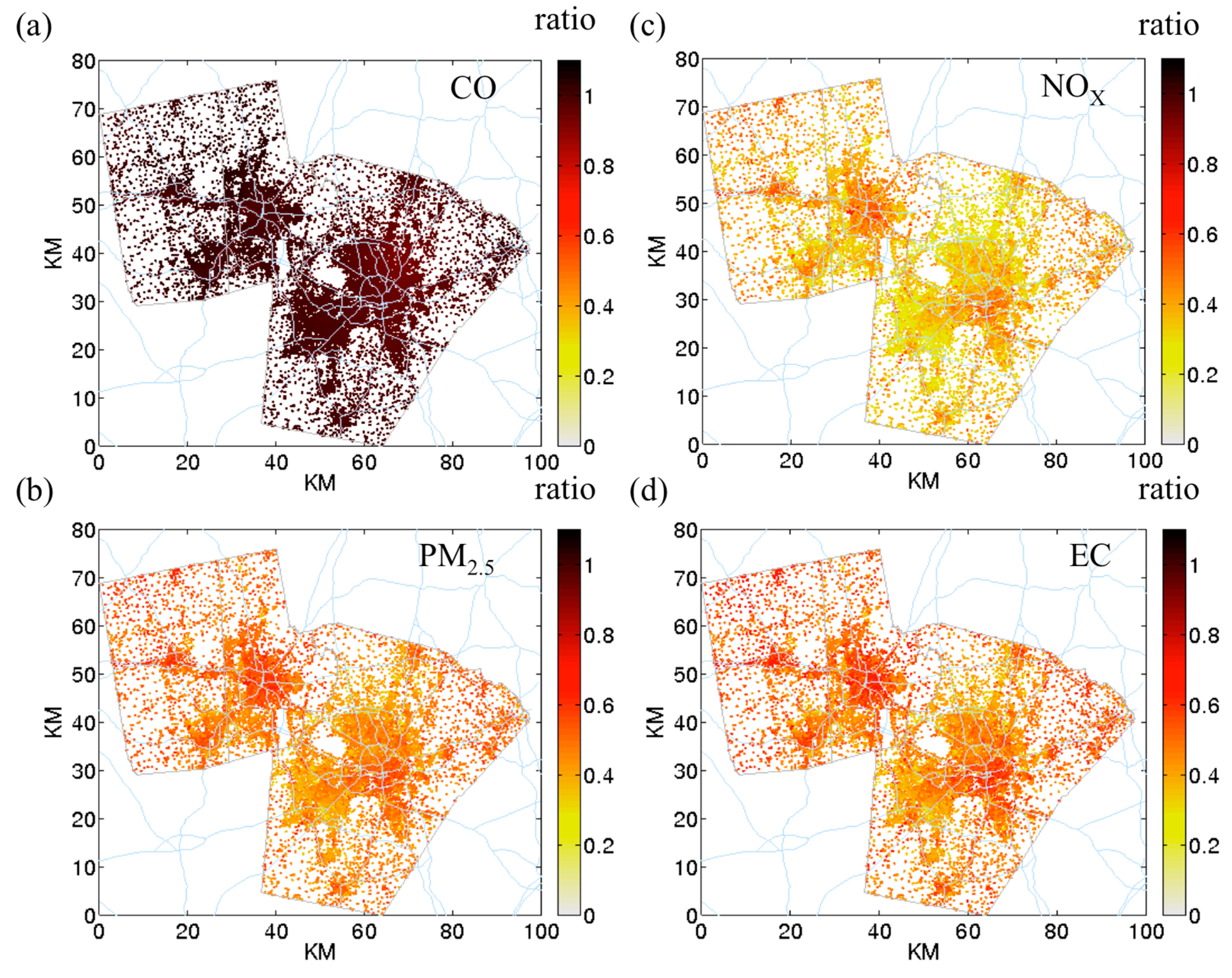
Figure 6 shows the concentration ratio at 07:00 between indoor and
outdoor hybrid concentration.
Figure 5.
Indoor concentration of CO and NOx at 07:00 with (a) CO indoor STOK; (b) NOx indoor STOK; (c) CO indoor hybrid; (d) NOx indoor hybrid. The color bar represents concentration in μg/m3 (Note that the color scale is different for the four figures to emphasize the concentration ranges that vary by pollutant).
For
PM2.5 and
EC (
Figure 6b,d), the ratio is ~0.7 and for
NOx (
Figure 6c), the ratio is ~0.5. The difference is because of the higher indoor deposition for
NOx (0.5 h
−1) compared to
PM2.5 (0.21 h
−1) and
EC (0.29 h
−1). The high ratio area overlaps with the area with high AER. High AER is seen mostly in urban area. As these areas usually have higher density of roadways, the residents have the potential to be exposed to higher air pollutant concentrations in the indoor environment.
Figure 6.
Indoor-outdoor concentration ratio using mean hybrid concentration at 07:00. (a) CO; (b) PM2.5; (c) NOx; and (d) EC.
Figure 6.
Indoor-outdoor concentration ratio using mean hybrid concentration at 07:00. (a) CO; (b) PM2.5; (c) NOx; and (d) EC.
The
spatial CV for
indoor STOK is higher than
outdoor STOK (
Figure 3 left panel). Because
outdoor STOK is homogenously distributed across space, pollutants with higher indoor deposition rate (
i.e.,
NOx,
PM2.5, and
EC) have a higher average
spatial CV in
indoor STOK than in
outdoor STOK. Compared to the
outdoor STOK, the average
spatial CV of the
indoor STOK is 3.6 fold higher for
NOx, 2.2 fold higher for
PM2.5, and 12.9 fold higher for
EC. As shown in
Figure 5b with the example for
NOx, this increase in spatial variability is from the spatial variation of AER.
Indoor on-road’s
spatial CV is not much different from
outdoor on-road. For
NOx,
PM2.5, and
EC, compared with the mean
spatial CV of the
outdoor on-road, the average
spatial CV of
indoor on-road changes less than 2%. Because the spatial variation for
outdoor on-road is large (
spatial CV ~2), the extra spatial variation from AER is “covered” and the
indoor on-road demonstrated similar
spatial CV to
outdoor on-road. For the
outdoor hybrid, the effect of infiltration on
spatial CV depends on the spatial variability of
outdoor hybrid. For
NOx and
EC, because the major contributor for
outdoor hybrid is
outdoor on-road, the
spatial CV of
outdoor hybrid is high (~0.8). Therefore, the
indoor hybrid shows only a slightly higher (10%)
spatial CV than the
outdoor hybrid for
NOx and
EC. For
PM2.5, because
outdoor STOK dominates the
outdoor hybrid, the
spatial CV of
outdoor hybrid is low (~0.17) the indoor infiltration produces the
indoor hybrid that has higher
spatial CV (40%) than the
outdoor hybrid.
Temporal CV in general, does not change much for STOK and hybrid between outdoor and indoor metrics (
Figure 3 right panel). For the on-road, due to the accumulation effect mentioned previously, the temporal variation is smoothed out, resulting in a lower temporal variation in indoor metrics than outdoor metrics.
3.3. The Overall Effect on Exposure Error
Because people spend more time indoors and STOK cannot capture the impact from a local source, we used the
indoor hybrid as a standard to compare to other metrics. To quantify the potential population exposure error using the other metrics, we created contingency tables [
33] for each pollutant that compares quintiles of the population exposure for the annual average concentration (
Table 3,
Table 4,
Table 5 and
Table 6). These tables’ diagonal values represent the percentage of Census blocks of a metric that agrees with the
indoor hybrid. With a perfect agreement with
indoor hybrid, the diagonal values would be 100% and the non-diagonal values would be 0. For example,
Table 3 shows the contingency table for
CO. Assuming the
indoor hybrid is closer to the actual exposure, the top left entry represents that of the population in the lowest quintile (~3200 Census blocks exposed to 347.4 to 362.1 μg/m
3 of
CO), the
outdoor hybrid metric correctly classified 91%. For
CO with the
outdoor hybrid, 9% of the Census blocks were grouped to the second lowest group. The high diagonal values for
CO for the
outdoor hybrid metric (>81%) indicate a good agreement between it and the
indoor hybrid. It is worth noting that the
outdoor STOK metric does not agree well with the
indoor hybrid (8% to 34% agreement).
Table 3.
Contingency table for CO showing agreement between exposure quintiles. The values represent percentage of Census blocks in each quintile. Concentration ranges are shown in parentheses. Boxed percentages along diagonals would be 100% for a perfect match.
Table 3.
Contingency table for CO showing agreement between exposure quintiles. The values represent percentage of Census blocks in each quintile. Concentration ranges are shown in parentheses. Boxed percentages along diagonals would be 100% for a perfect match.
| | Percentile | Concentration (μg/m3) | Indoor Hybrid |
|---|
| 0–20 | 20–40 | 40–60 | 60–80 | 80–100 |
|---|
| (347.4, 362.1) | (362.1, 372.0) | (372.0, 385.4) | (385.4, 411.6) | (411.6, 2242.2) |
|---|
| Outdoor hybrid | 0%–20% | (330.2, 345.9) | 91 | 10 | 0 | 0 | 0 |
| 20%–40% | (345.9, 353.9) | 9 | 81 | 11 | 0 | 0 |
| 40%–60% | (353.9, 365.7) | 0 | 9 | 85 | 6 | 0 |
| 60%–80% | (365.7, 388.0) | 0 | 0 | 4 | 92 | 3 |
| 80%–100% | (388.0, 2024.4) | 0 | 0 | 0 | 2 | 97 |
| Indoor on-road | 0%–20% | (6.7, 25.2) | 79 | 21 | 0 | 0 | 0 |
| 20%–40% | (25.2, 35.4) | 15 | 64 | 21 | 0 | 0 |
| 40%–60% | (35.4, 49.2) | 6 | 13 | 70 | 11 | 0 |
| 60%–80% | (49.2, 76.6) | 0 | 2 | 9 | 83 | 6 |
| 80%–100% | (76.6, 1903.4) | 0 | 0 | 0 | 6 | 94 |
| Outdoor on-road | 0%–20% | (5.8, 21.3) | 78 | 23 | 0 | 0 | 0 |
| 20%–40% | (21.3, 30.0) | 16 | 61 | 24 | 0 | 0 |
| 40%–60% | (30.0, 42.2) | 6 | 14 | 66 | 13 | 0 |
| 60%–80% | (42.2, 66.5) | 0 | 2 | 10 | 82 | 6 |
| 80%–100% | (66.5, 1694.4) | 0 | 0 | 0 | 5 | 94 |
| Indoor STOK | 0%–20% | (317.2, 336.1) | 25 | 16 | 12 | 22 | 25 |
| 20%–40% | (336.1, 339.3) | 10 | 18 | 18 | 23 | 30 |
| 40%–60% | (339.3, 341.3) | 12 | 27 | 30 | 17 | 14 |
| 60%–80% | (341.3, 343.7) | 6 | 16 | 26 | 29 | 23 |
| 80%–100% | (343.7, 347.7) | 47 | 22 | 14 | 9 | 8 |
| Outdoor STOK | 0%–20% | (322.3, 337.6) | 24 | 16 | 12 | 22 | 27 |
| 20%–40% | (337.6, 340.7) | 12 | 18 | 18 | 24 | 28 |
| 40%–60% | (340.7, 342.2) | 8 | 27 | 34 | 17 | 15 |
| 60%–80% | (342.2, 343.7) | 8 | 17 | 23 | 29 | 22 |
| 80%–100% | (343.7, 347.7) | 48 | 23 | 13 | 8 | 8 |
For
NOx and
EC (
Table 4 and
Table 6), the
outdoor hybrid does not perform well (the agreement is between 33% and 49% for the lower four groups) except for the highest quintile (73% for
NOx and 76% for
EC). All the other outdoor metrics for
NOx and
EC perform poorly (
Table 4,
Table 5 and
Table 6). The best agreement for
NOx and
EC is with the
indoor on-road (agreement between 45% and 90%). At the lowest quintile,
indoor STOK performs well (68% for
NOx and 69 for
EC).
For
PM2.5 (
Table 5),
indoor STOK performs the best (agreement between 59% and 90%). All other metrics perform poorly. For all pollutants in general, all outdoor metrics perform relatively poorer than indoor metrics.
Outdoor STOK, in specific, performs very poorly (agreement ranges from 8% to 34% considering all pollutants). Since space-time kriging is often used in environmental health studies to quantify air pollutant exposures [
13,
14,
15], this part of analysis shows that there is a great potential for this metric to misclassify exposures for all four pollutants studied.
Table 4.
Contingency table for NOx showing agreement between exposure quintiles. The values represent percentage of Census blocks in each quintile. Concentration ranges are shown in parentheses. Boxed percentages along diagonals would be 100% for a perfect match.
Table 4.
Contingency table for NOx showing agreement between exposure quintiles. The values represent percentage of Census blocks in each quintile. Concentration ranges are shown in parentheses. Boxed percentages along diagonals would be 100% for a perfect match.
| | Percentile | Concentration (μg/m3) | Indoor Hybrid |
|---|
| 0–20 | 20–40 | 40–60 | 60–80 | 80–100 |
|---|
| (3.4, 9.3) | (9.3, 11.1) | (11.1, 13.5) | (13.5, 17.7) | (17.7, 307.9) |
|---|
| Outdoor hybrid | 0%–20% | (18.4, 23.3) | 49 | 31 | 17 | 3 | 0 |
| 20%–40% | (23.3, 25.4) | 32 | 34 | 25 | 10 | 0 |
| 40%–60% | (25.4, 28.6) | 13 | 26 | 33 | 26 | 1 |
| 60%–80% | (28.6, 35.1) | 4 | 8 | 20 | 41 | 26 |
| 80%–100% | (35.1, 594.7) | 1 | 1 | 4 | 20 | 73 |
| Indoor on-road | 0%–20% | (0.5, 2.6) | 69 | 26 | 5 | 0 | 0 |
| 20%–40% | (2.6, 3.7) | 28 | 49 | 22 | 2 | 0 |
| 40%–60% | (3.7, 5.3) | 3 | 24 | 55 | 18 | 0 |
| 60%–80% | (5.3, 8.9) | 0 | 1 | 18 | 70 | 10 |
| 80%–100% | (8.9, 299.0) | 0 | 0 | 0 | 10 | 90 |
| Outdoor on-road | 0%–20% | (1.7, 6.1) | 49 | 32 | 17 | 3 | 0 |
| 20%–40% | (6.1, 8.3) | 33 | 33 | 26 | 9 | 0 |
| 40%–60% | (8.3, 11.4) | 13 | 26 | 33 | 26 | 1 |
| 60%–80% | (11.4, 18.0) | 4 | 8 | 20 | 42 | 25 |
| 80%–100% | (18.0, 577.4) | 1 | 1 | 4 | 20 | 73 |
| Indoor STOK | 0%–20% | (2.4, 6.5) | 68 | 18 | 6 | 4 | 4 |
| 20%–40% | (6.5, 7.3) | 22 | 40 | 20 | 11 | 8 |
| 40%–60% | (7.3, 8.2) | 9 | 26 | 31 | 21 | 13 |
| 60%–80% | (8.2, 9.3) | 2 | 13 | 30 | 31 | 24 |
| 80%–100% | (9.3, 14.4) | 0 | 2 | 13 | 33 | 52 |
| Outdoor STOK | 0%–20% | (18.9, 19.0) | 22 | 23 | 24 | 18 | 14 |
| 20%–40% | (19.0, 19.3) | 13 | 16 | 19 | 22 | 30 |
| 40%–60% | (19.3, 19.3) | 16 | 15 | 16 | 20 | 31 |
| 60%–80% | (19.3, 19.4) | 18 | 21 | 21 | 26 | 14 |
| 80%–100% | (19.4, 20.2) | 31 | 25 | 21 | 14 | 10 |
Table 5.
Contingency table for PM2.5 showing agreement between exposure quintiles. The values represent percentage of Census blocks in each quintile. Concentration ranges are shown in parentheses. Boxed percentages along diagonals would be 100% for a perfect match.
Table 5.
Contingency table for PM2.5 showing agreement between exposure quintiles. The values represent percentage of Census blocks in each quintile. Concentration ranges are shown in parentheses. Boxed percentages along diagonals would be 100% for a perfect match.
| | Percentile | Concentration (μg/m3) | Indoor Hybrid |
|---|
| 0–20 | 20–40 | 40–60 | 60–80 | 80–100 |
|---|
| (1.72, 4.03) | (4.03, 4.45) | (4.45, 4.83) | (4.83, 5.28) | (5.28, 21.21) |
|---|
| Outdoor hybrid | 0%–20% | (7.91, 8.43) | 27 | 24 | 22 | 19 | 8 |
| 20%–40% | (8.43, 8.79) | 27 | 21 | 20 | 19 | 13 |
| 40%–60% | (8.79, 8.90) | 26 | 27 | 23 | 15 | 10 |
| 60%–80% | (8.90, 9.17) | 15 | 19 | 22 | 24 | 20 |
| 80%–100% | (9.17, 34.29) | 6 | 8 | 13 | 23 | 50 |
| Indoor on-road | 0%–20% | (0.03, 0.15) | 42 | 26 | 20 | 10 | 2 |
| 20%–40% | (0.15, 0.21) | 34 | 30 | 19 | 13 | 5 |
| 40%–60% | (0.21, 0.29) | 16 | 27 | 28 | 22 | 8 |
| 60%–80% | (0.29, 0.47) | 7 | 13 | 24 | 31 | 26 |
| 80%–100% | (0.47, 16.33) | 2 | 4 | 11 | 23 | 60 |
| Outdoor on-road | 0%–20% | (0.07, 0.26) | 28 | 26 | 24 | 17 | 6 |
| 20%–40% | (0.26, 0.34) | 33 | 27 | 20 | 15 | 6 |
| 40%–60% | (0.34, 0.47) | 22 | 25 | 23 | 20 | 9 |
| 60%–80% | (0.47, 0.74) | 12 | 14 | 20 | 25 | 29 |
| 80%–100% | (0.74, 26.00) | 5 | 8 | 13 | 23 | 51 |
| Indoor STOK | 0%–20% | (1.67, 3.85) | 90 | 8 | 1 | 1 | 1 |
| 20%–40% | (3.85, 4.21) | 11 | 73 | 11 | 3 | 2 |
| 40%–60% | (4.21, 4.53) | 0 | 19 | 62 | 14 | 5 |
| 60%–80% | (4.53, 4.89) | 0 | 0 | 25 | 59 | 16 |
| 80%–100% | (4.89, 6.55) | 0 | 0 | 0 | 24 | 76 |
| Outdoor STOK | 0%–20% | (8.46, 8.61) | 15 | 16 | 18 | 23 | 27 |
| 20%–40% | (8.61, 8.69) | 32 | 27 | 22 | 12 | 7 |
| 40%–60% | (8.69, 8.72) | 15 | 15 | 17 | 22 | 31 |
| 60%–80% | (8.72, 8.76) | 18 | 19 | 20 | 23 | 20 |
| 80%–100% | (8.76, 9.14) | 20 | 23 | 23 | 20 | 14 |
Table 6.
Contingency table for EC showing agreement between exposure quintiles. The values represent percentage of Census blocks in each quintile. Concentration ranges are shown in parentheses. Boxed percentages along diagonals would be 100% for a perfect match.
Table 6.
Contingency table for EC showing agreement between exposure quintiles. The values represent percentage of Census blocks in each quintile. Concentration ranges are shown in parentheses. Boxed percentages along diagonals would be 100% for a perfect match.
| | Percentile | Concentration (μg/m3) | Indoor Hybrid |
|---|
| 0–20 | 20–40 | 40–60 | 60–80 | 80–100 |
|---|
| (0.15, 0.37) | (0.37, 0.43) | (0.43, 0.50) | (0.50, 0.62) | (0.62, 12.74) |
|---|
| Outdoor hybrid | 0%–20% | (0.65, 0.74) | 49 | 32 | 17 | 2 | 0 |
| 20%–40% | (0.74, 0.79) | 32 | 35 | 27 | 7 | 0 |
| 40%–60% | (0.79, 0.86) | 14 | 25 | 34 | 26 | 1 |
| 60%–80% | (0.86, 1.01) | 4 | 7 | 19 | 46 | 23 |
| 80%–100% | (1.01, 19.61) | 1 | 1 | 3 | 18 | 76 |
| Indoor on-road | 0%–20% | (0.02, 0.09) | 65 | 28 | 7 | 0 | 0 |
| 20%–40% | (0.09, 0.12) | 30 | 45 | 23 | 2 | 0 |
| 40%–60% | (0.12, 0.17) | 5 | 25 | 52 | 18 | 0 |
| 60%–80% | (0.17, 0.28) | 0 | 2 | 18 | 69 | 11 |
| 80%–100% | (0.28, 12.38) | 0 | 0 | 0 | 11 | 89 |
| Outdoor on-road | 0%–20% | (0.04, 0.15) | 48 | 32 | 18 | 2 | 0 |
| 20%–40% | (0.15, 0.20) | 33 | 34 | 26 | 8 | 0 |
| 40%–60% | (0.20, 0.28) | 14 | 25 | 33 | 26 | 1 |
| 60%–80% | (0.28, 0.43) | 5 | 7 | 19 | 45 | 23 |
| 80%–100% | (0.43, 19.00) | 1 | 1 | 3 | 18 | 76 |
| Indoor STOK | 0%–20% | (0.11, 0.27) | 69 | 17 | 6 | 4 | 4 |
| 20%–40% | (0.27, 0.30) | 22 | 41 | 18 | 11 | 9 |
| 40%–60% | (0.30, 0.33) | 8 | 26 | 30 | 20 | 15 |
| 60%–80% | (0.33, 0.36) | 1 | 13 | 31 | 29 | 25 |
| 80%–100% | (0.36, 0.49) | 0 | 2 | 15 | 36 | 47 |
| Outdoor STOK | 0%–20% | (0.55, 0.55) | 13 | 20 | 22 | 22 | 23 |
| 20%–40% | (0.55, 0.55) | 10 | 15 | 17 | 22 | 36 |
| 40%–60% | (0.55, 0.55) | 31 | 26 | 24 | 13 | 6 |
| 60%–80% | (0.55, 0.56) | 14 | 16 | 20 | 26 | 23 |
| 80%–100% | (0.56, 0.56) | 31 | 23 | 18 | 16 | 12 |
Besides the population exposure error, it is also important to quantify the exposure error at an individual level. We quantify this with
ND (
Figure 7 left panel) and
NAD (
Figure 7 right panel). For all pollutants except for
CO, all outdoor metrics (dark boxes) perform poorly. For example, the average
ND and
NAD is 175% with the
outdoor hybrid for
NOx. Further, all outdoor metrics have shown wider 90% range (
Figure 7 whiskers); so for some Census block,
ND and
NAD can be up to 375% for
NOx. From the population exposure error in the previous paragraph, one would expect that the
indoor on-road would perform better for
NOx and
EC. However, for these two pollutants,
ND and
NAD indicate that
indoor STOK yields lower error (average
ND ~−25% and
NAD ~25%) compared to
indoor on-road (average
ND ~−75% and
NAD ~75%). The disagreement between population and individual exposure error is because although the
indoor on-road can capture the locations of the hotspot, the concentration is still too low to represent the true exposure. For
CO, the best performance is with
outdoor hybrid metric (average
ND ~0% and
NAD ~10%). Because the penetration factor for
CO is 1 and the indoor deposition rate is 0, the indoor and outdoor concentration differ less from each other, although
NAD can still be up to 30% (
Figure 7). For
PM2.5, agreeing with the population exposure, the
indoor STOK concentration gives the lowest error (average
ND ~0% and
NAD ~5%). This is because of the relatively lower contribution from the on-road source for
PM2.5. However, it is worth noting that the error can sometimes be large (up to 25%), indicating on-road source still plays an important role for the near-road population exposure.
Figure 7.
Hourly normalized difference (ND, left panels) and hourly normalized absolute difference (NAD, right panels) for each Census block for CO (a,e); NOx (b,f); PM2.5 (c,g); and EC (d,h). Bottom and top of box represents 25th and 75th percentiles, the line in the middle of the box is the median, the ends of the whisker are the 5th and 95th percentiles, and the dot on the whisker is the mean.


 ,
, 

